Long Range Transport of Southeast Asian PM2.5 Pollution to Northern Thailand during High Biomass Burning Episodes

Abstract

This paper aims to investigate the potential contribution of biomass burning in PM2.5 pollution in Northern Thailand. We applied the coupled atmospheric and air pollution model which is based on the Weather Research and Forecasting Model (WRF) and a Hybrid Single-Particle Lagrangian Integrated Trajectory Model (HYSPLIT). The model output was compared to the ground-based measurements from the Pollution Control Department (PCD) to examine the model performance. As a result of the model evaluation, the meteorological variables agreed well with observations using the Index of Agreement (IOA) with ranges of 0.57 to 0.79 for temperature and 0.32 to 0.54 for wind speed, while the fractional biases of temperature and wind speed were 1.3 to 2.5 °C and 1.2 to 2.1 m/s. Analysis of the model and hotspots from the Moderate Imaging Spectroradiometer (MODIS) found that biomass burning from neighboring countries has greater potential to contribute to air pollution in northern Thailand than national emissions, which is indicated by the number of hotspot locations in Burma being greater than those in Thailand by two times under the influence of two major channels of Asian Monsoons, including easterly and northwesterly winds that bring pollutants from neighboring counties towards northern Thailand.

1. Introduction

Air pollution is a widespread problem that affects human health and other atmospheric aspects, i.e., it can contribute to the warming of the atmosphere and can affect rain and cloud patterns. Air pollution is released from a number of man-made and natural sources including fossil fuels burning in electricity production, transportation, industry and households, agriculture, and waste processing. According to a 2014 World Health Organization (WHO) report the premature deaths of about 7 million people worldwide were caused by air pollution [1]. It is estimated that in developing countries approximately 300,000 to 700,000 people can be saved from premature death if aerosol levels are reduced to a safe level (an Air Quality Index (AQI) number under 100 signifies good or acceptable air quality) [2].

Southeast Asia is a region with frequent air pollution problems every year, particularly at the beginning of the year, from January to April. Biomass burning strongly dominates air pollution from the regional to local scale in Southeast Asia [3]. Moreover, severe haze events in this region caused by particulate pollution have become more intense and frequent in recent years. Widespread biomass burning occurrences and particulate pollutants from human activities other than biomass burning play important roles in degrading the air quality in Southeast Asia [4,5]. In addition, appropriate meteorological and topographic effects are also favorable conditions that contribute to the air pollution problem in Southeast Asia. In northern Thailand, all these factors are combined. Most cities in northern Thailand are located in the mountainous area and surrounded by paddy fields. Larger villages like Chiang Mai face increasing problems due to traffic jams, but farmers also burn stubble in preparation for the coming rain and rice planting at this time of the year, and these narrow valleys provide perfect bowls for this smog and smoke.

The contributing pollutants in Northern Thailand, however, are not only from national sources but also from long-distance air pollutants introduced by meteorological factors, i.e., wind, temperature, and humidity [6,7,8,9]. The climate of northern Thailand is characterized by monsoons. The period from mid-February until the end of May is the transition period from Northeast monsoon (most prevalent in December–January) to Southwest monsoon (most prevalent in July–August) climates. The hottest weather observed during March–April, coinciding with the presence of intensive thermal lows in the area [10]. During the transition period, winds can transport air pollutants from the surrounding area into northern Thailand [11]. The northeastern monsoon transfers air pollutants from China to the southern Chinese sea from mid-December to mid-April and can then flow continuously to the mainland Southeast Asia.

Exposure to high levels of air pollution can cause a variety of adverse health outcomes. PM2.5 is the most important air pollutant and strongly affects human health. Recent calculations of global premature mortality rates on the basis of high-resolution global O3 and PM2.5 models show that Southeast Asia and the Western Pacific account for around 25% and 45% of world mortality [12,13]. PM2.5 can penetrate deeply into the respiratory tract and enter the lungs. Exposure to small particles can also impair the function of the lungs and exacerbate medical conditions such as asthma and heart disease [14,15,16]. At the beginning of 2020, the PM2.5 measurements of air pollution in Chiang Mai, one of the largest cities in northern Thailand, reached a staggering level of 330 on the PM2.5 concentration over the weekend, making the northern city the most polluted city in the world, while the airborne pollution levels across Thailand’s northern region vary between 100 and 390 of the air pollutants concentrations, according to AirVisual data. There have been a few studies exploring the source contributions of PM2.5 in this region. For example, Chueinta et al. [17] reported the characterization and source identification of fine and coarse particles collected in urban and suburban residential areas in Thailand and later performed an extended study on the Bangkok metropolitan curbside [18]. Leenanupan et al. [19] carried out similar work on the characterization of fine particulate pollution in the Mae Hong Son province in the north of Thailand. A few collaborative studies on fine and coarse particulate air pollution at the Asia Pacific regional scale were also reported, e.g., Oanh et al. [6,7]; Ebihara et al. [20,21]; Hopke et al. [22]. Moreover, only a few long-term PM2.5 and PM_10–2.5 monitoring data are available for elsewhere in this region. However, it is unclear how much neighboring countries contribute to the air pollution problem in northern Thailand. In addition, Lee et al. [5] found that nitrate aerosol was the major component of PM2.5 particles in Southeast Asia.

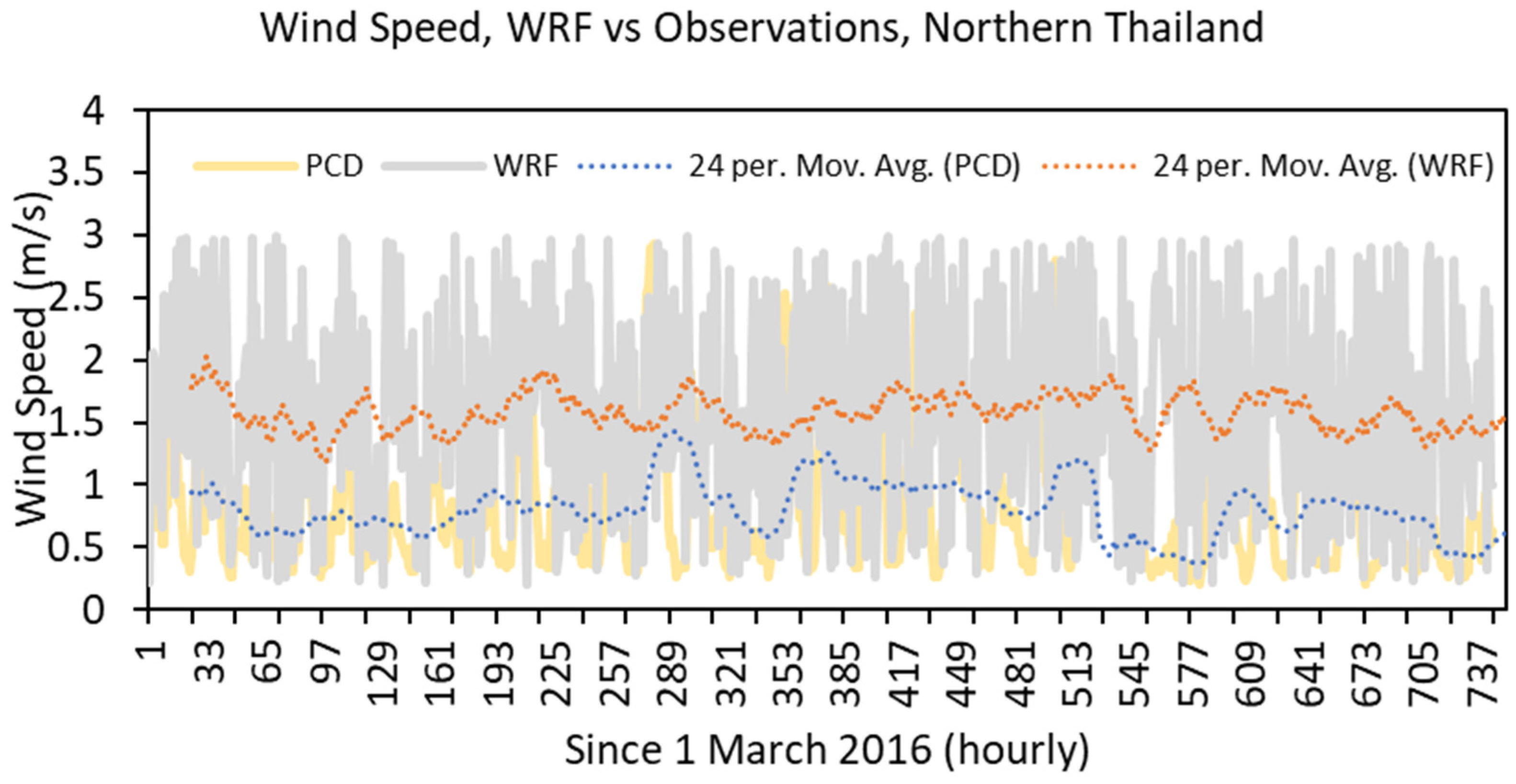
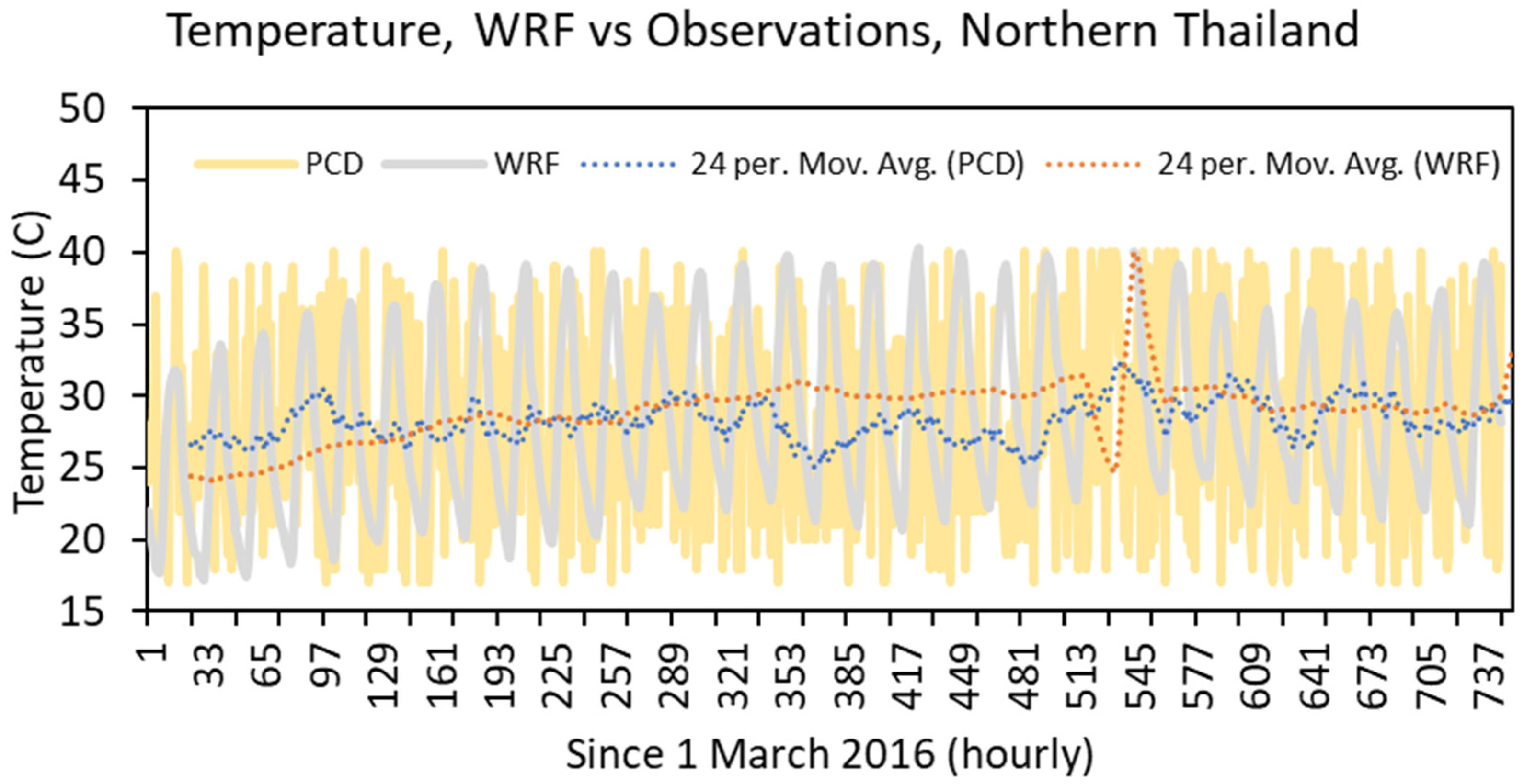
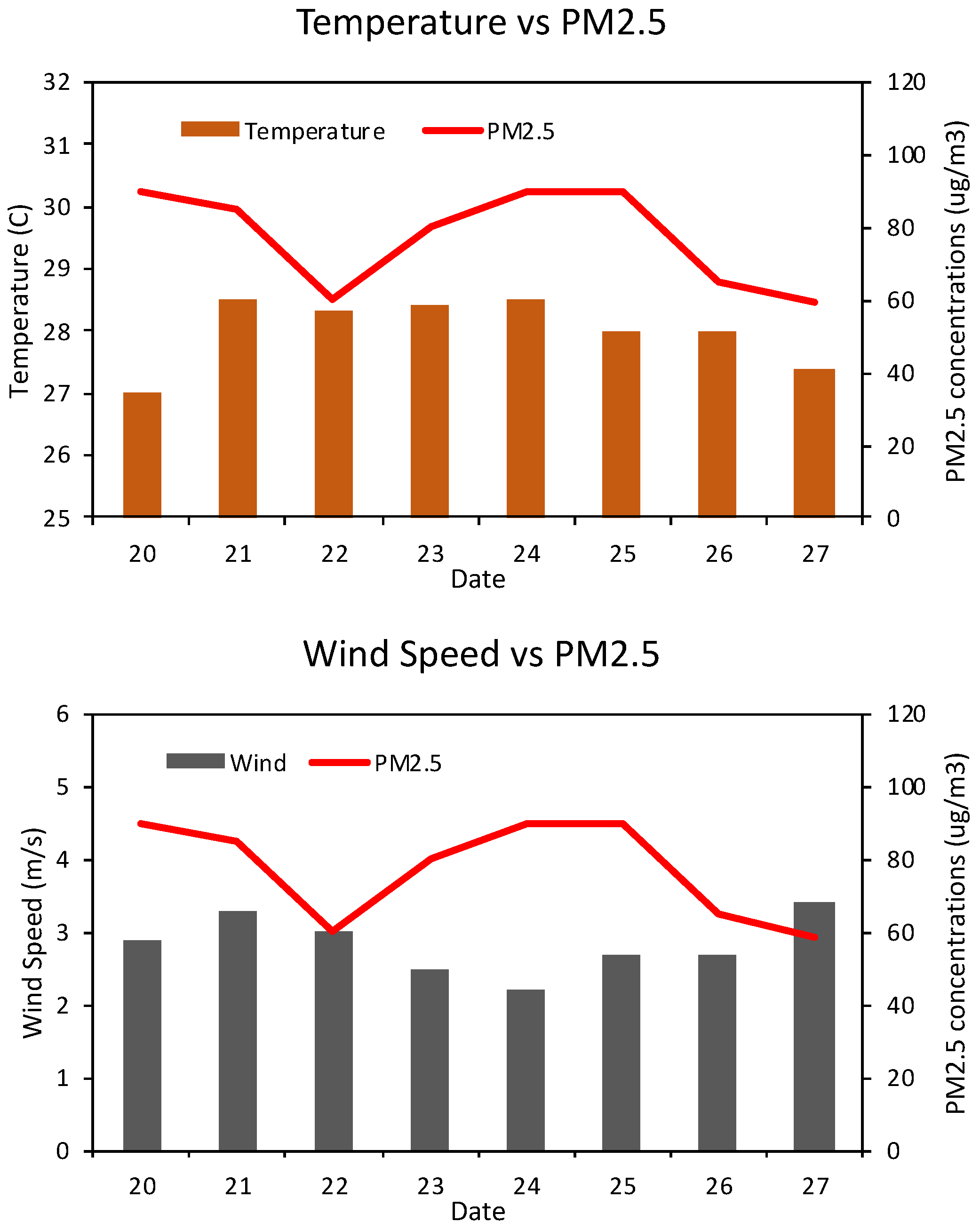
This work applied atmospheric model coupling with the air pollution model to investigate the potential contributions of biomass burning in air pollution in Northern Thailand. We used the Weather Research and Forecasting (WRF) model version 3.8.1 to simulate the meteorological conditions on March 2016. The model’s initial and boundary conditions were taken from the Final Analysis Data (FNL) [23], and the modeled temperature and wind speed were compared to a dataset from the Pollution Control Department (PCD). To clarify the model’s capabilities, statistical analyses such as Index of Agreement (IOA) and Fractional Bias FB were used for the model evaluation. The output from the WRF model was used as the meteorological conditions to be inserted into the Hybrid Single-Particle Lagrangian Integrated Trajectory (HYSPLIT) model to determine the long-range transport of regional air pollutants from the neighboring countries of Southeast Asia toward northern Thailand.

2. Materials and Methods

We use a coupled atmospheric model called the WRF model version 3.8 [24] to generate the meteorological input for HYSPLIT, which is an air quality model. The results from HYSPLIT were then used to identify the PM2.5 pathway in Southeast Asia.

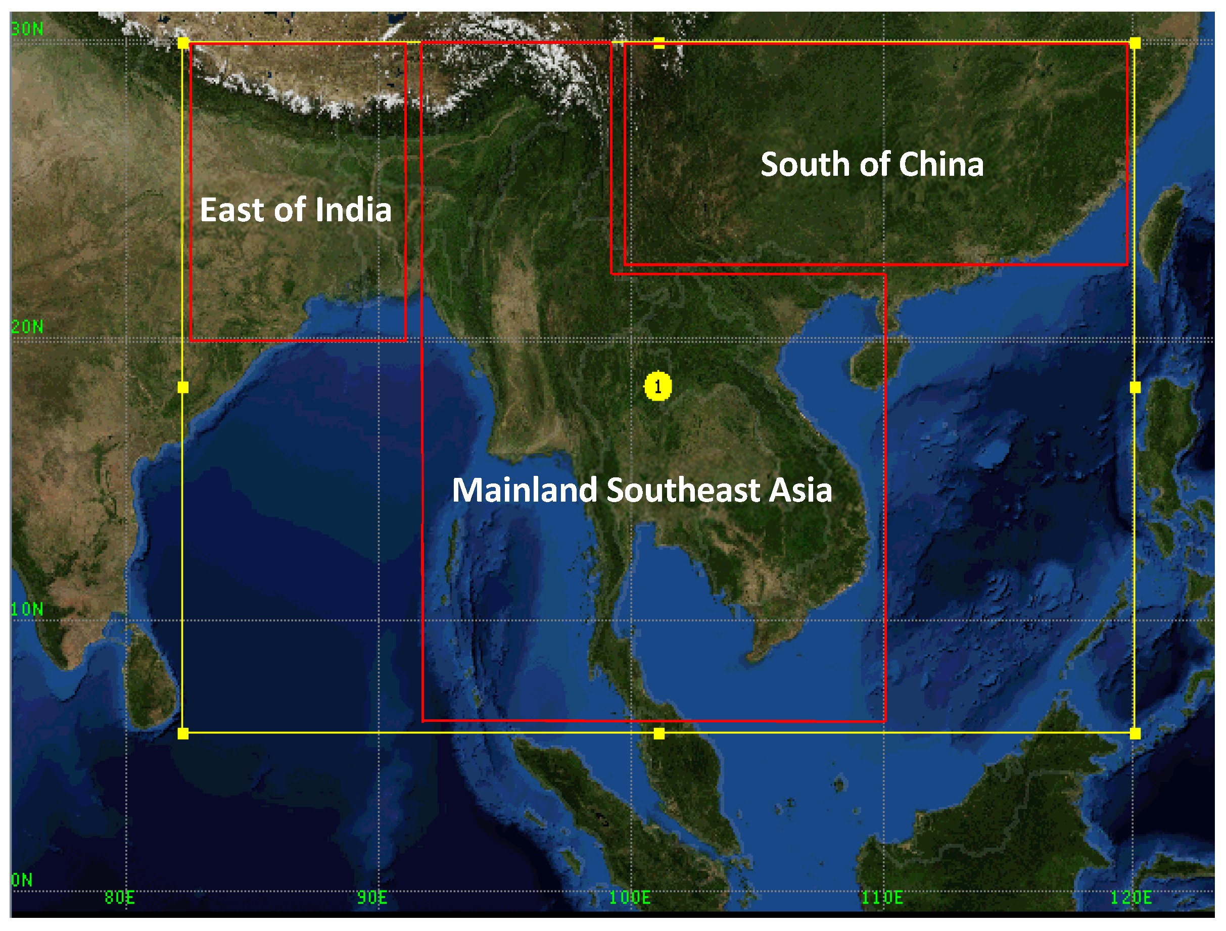
The WRF model was developed to study several atmospheric factors and also to be used for operational weather forecasting. It is a non-hydrostatic mesoscale model consisting of several physical schemes, including radiation, cumulus, and microphysics. In this study, we designed 1 WRF domain with a horizontal resolution of 20 km grid spacing. In addition, the model sets 30 vertical levels up to 50 hPa. The outer domain entirely covers the upper mainland of Southeast Asia and some areas of East and South Asia, such as the South of China and East of India, as shown in Figure 1. The model configuration was listed in

Table 1. Physics option in model configuration.

Scheme	Option
Microphysics	WRF Single Moment (WSM) 3-class simple ice scheme
Radiation	rrtm scheme
Surface Phyaics	Duhia
Land Surface Model	Noah Land Surface Model
Convective	Kain–Fritsch (new Eta) scheme

. Southeast Asia is influenced by East Asian monsoons, which carry the air mass from high latitudes to this region. The transboundary transport from the western border, such as Myanmar and India, also affect the quality of the air in northern Thailand, while the inner domain is located in northern Thailand. To solve the water vapor, cloud, and precipitation process, the model was configured using the WRF Single-Moment 3-class scheme according to Hong et al. [25]; Hong and Lim [26]. This method predicts a simple-ice system with three types of hydrometers: vapor, cloud water, and rain. The calculation of these processes is based on the mass content of the diagnostic relationship. The Kain–Fritsch scheme [27] is the sub-grid scale process used for the convective resolution. It has the potential to use a cloud model with updrafts and downdrafts, as well as to consider the effects of detrainment and training on cloud formation. The similarity theory scheme is used to emulate the thermal gradient over the surface responsible for friction velocity and wind over the surface [28,29,30,31,32]. The model spin-up was conducted from 15 to 28 February 2012 to reduce the effects from the initial conditions. From 1 March 2012 to 1 April 2012, the WRF model was designed to simulate the weather conditions for the HYSPLIT model. The main meteorological variables of the WRF model, i.e., wind (U, V, W), temperature (T), surface pressure (Psfc), and relative humidity (RH), were used as input data for the HYSPLIT model.

The HYSPLIT model [33] is designed to calculate both simple air plot pathways and complex dispersal and deposition simulations. This model is used to determine air pollutants in source–receptor relationships through trajectory analyses and predict dispersion for a number of events, such as volcanic eruptions, the transportation of wildfire smoke, and episodes of dust storms (http:/ready.arl.noaa.gov/index.php). HYSPLIT is a Lagrangian model, meaning that its scatter calculations follow the vector of transport, and only the computing point meteorological fields are required. HYSPLIT has the same horizontal coordination and map projections as the meteorological input. The meteorological profiles for the vertical grid are interpolated linearly onto an internal model following the field coordination. Particles released from a source are advected by a mid-wind field in a particle dispersion simulation and dispersed according to the random components caused by atmospheric turbulence. The meteorological data fields of each meteorological input source are then converted from (Gridded Binary (GRIB1 and GRIB2), netCDF, MM5, etc.) to a common format required for the running of HYSPLIT. Typically, 1 or 3 h weather data are the most commonly used for the calculation of transport and dispersion and are then temporarily interpolated linearly between the input data times to the HYSPLIT integration time.

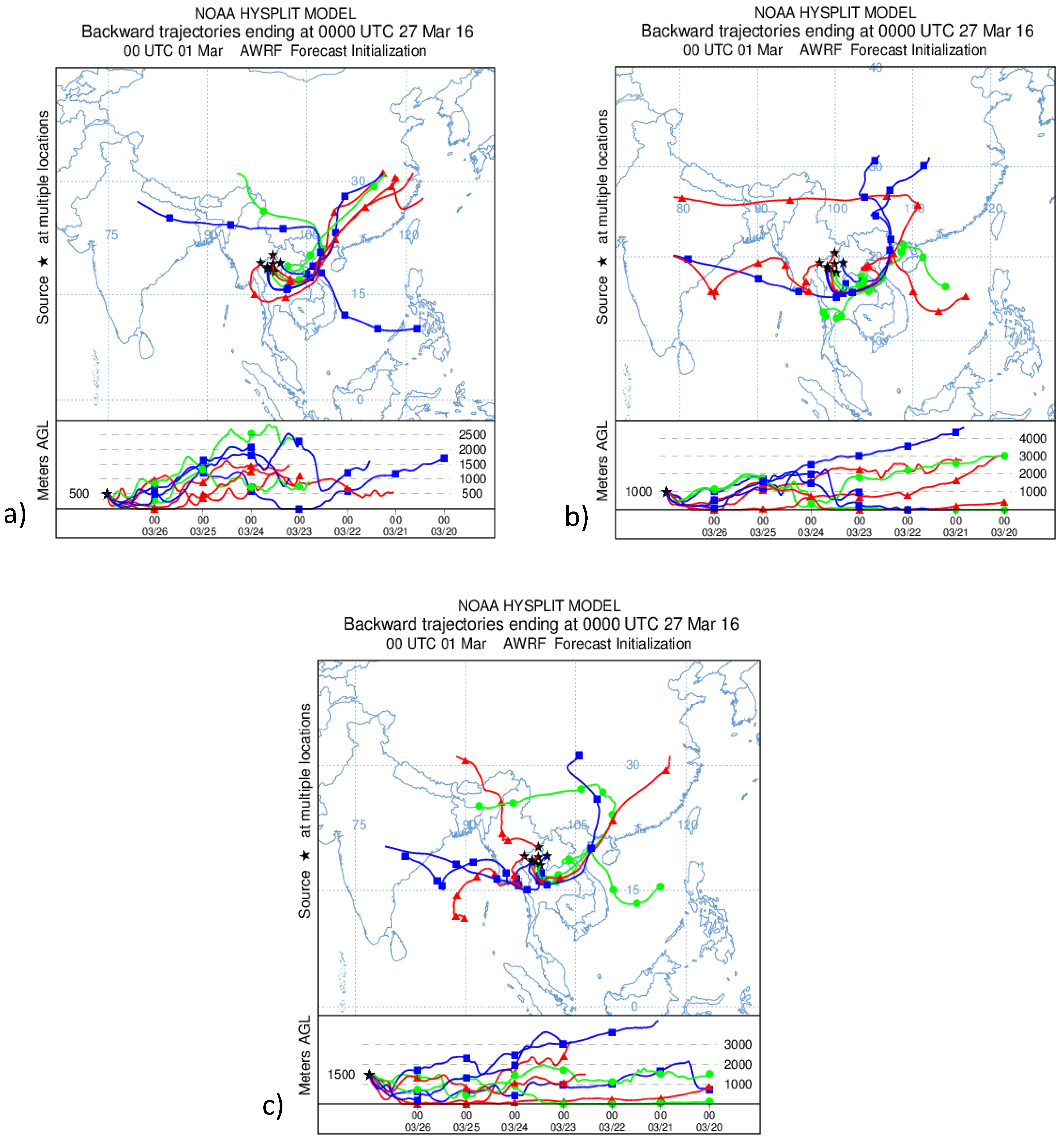
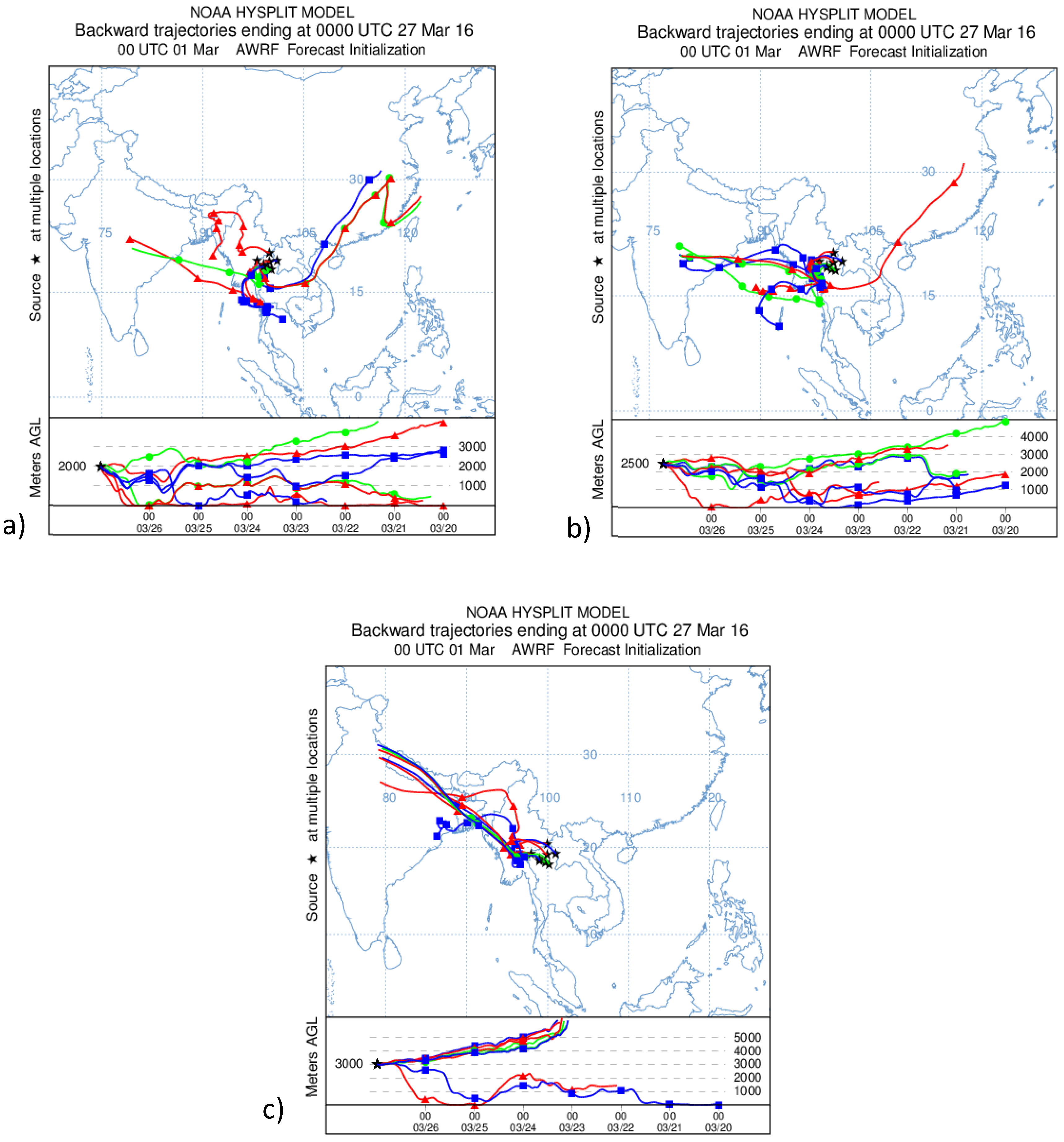
The HYSPLIT model was driven to produce back trajectories of parcels originating from an observational site via the above-described WRF simulation atmospheric fields. The backward trajectory provides the Lagrangian paths of the air parcels within the timeframe chosen (24 h in the current study). This path is useful for identifying the source locations of the pollutants that fall within the backward trajectory. Based on the PM2.5 concentrations in 8 observation sites in northern Thailand in March, the maximum PM2.5 concentration for the back-trajectory analysis was found on 27 March 2012. Once the sources were identified, the HYSPLIT model was applied to each of the identified sites for a 24-h period. The computer domain in HYSPLIT was designed to have a horizontal grid of 300 to 300 cells, each with a resolution of 0.01° and eight vertical levels (500, 1000, 1500, 2000, 2500, and 3000 m above ground level). A full 3D dispersion particulate model with a total of 5000 particles released for each emission cycle was used. The speed of the horizontal and vertical turbulence was calculated using the Kantha and Clayson method [34]. The stability of the boundary layer was estimated by heat and momentum, and the mixed depth of the layer was derived from the meteorological model.

3. Results and Discussion

3.1. Meteorological and Trajectory Modelling

To analyze the potential contribution of biomass burning in air pollution in Northern Thailand, the meteorological conditions and tracing of the dispersed emission sources due to biomass burning from many locations are required. In this paper, we use the Lagrange particle dispersion model known as Hybrid Single-particle Lagrangian Integrated Trajectory (HYSPLIT) with meteorological data from the WRF simulation in March 2016 to determine the transport of particle air parcels. A Lagrangian approach was chosen here as this approach is suitable to study the transboundary transport of particles with backward trajectories of air parcels across the Southeast Asian region due to biomass burning during the dry season. In addition, we used the output from the WRF model to analyze the meteorological patterns in March 2016.

3.1.1. Meteorological Model Evaluation

Since we used the WRF simulation output to analyze the meteorological patterns and input the data into HYSPLIT, the model output needs to be evaluated by comparing the output with actual data from ground-based measurements. We compared the model results from the WRF model to the ground-based observations from the Pollution Control Department (PCD), as shown in

Table 2. Location of the Pollution Control Department (PCD) measurements in northern Thailand.

Location	Latitude	Longitude
Nan	18.78	100.77
Lampang	18.25	99.76
Chiang Mai	18.78	98.98

. In general, the Thai PCD measures the hourly concentrations of six pollutants: PM₁₀, PM2.5, CO, NO₂, SO₂, and O₃. The PCD measurement sites are located near urban areas, so the results are likely to be influenced by the emissions of motor vehicles. Since the PCD recently measured PM2.5 in Thailand, some station sites offer a PM2.5 dataset. Here, we compared the modeled results to the PCD dataset at 3 locations, based on the complete PM2.5 dataset shown in

Table 3. Statistical analysis between the Weather Research and Forecasting (WRF) model and ground-based measurements.

Station	Temperature		Wind Speed
	The Index of Agreement (IOA)	Fractional Bias (FB)	IOA	FB
Chiang Mai	0.79	2.5	0.54	2.1
Lampang	0.66	1.3	0.46	1.5
Nan	0.57	2.4	0.32	1.2

. We used the statistical indicators, the Index of Agreement (IOA) and Fractional Bias (FB), to examine the efficiency of the model.

A comparison between the hourly output of the model and the observational data is shown in Figure 2. In general, the model results accurately reflected the real observations. The modeled temperature at 2 m was slightly higher than the ground-based measurements by 2–3 °C, while the wind speed was overestimated by 1 m/s. In addition, the statistical analysis shown in Table 3 indicates that the WRF and PCD datasets agree well in the hourly temperature and wind speed for most sites, with an acceptable IOA in the range of 0.57 to 0.79 for temperature and 0.32 to 0.54 for wind speed. However, the model generally overestimated the temperature by 1.3–2.5 °C and the temperature by 1.2–2.1 m/s, as indicated by Fractional Bias (FB). These errors are most likely to be caused by the rough resolution of the 20 km grid spacing model simulation, which has difficulty simulating sub-grid scale processes, such as convection and wind. In particular, the simulation of wind requires correction of the Large Eddy Simulation (LES). As discussed in Wurps et al. [35], a good LES simulation corresponds to a very fine resolution, such as 2.5 m, 10 m, and 20 m.

3.1.2. General Meteorology

The general meteorological conditions for the month of March 2016 in Southeast Asia can be better understood by analyzing the wind flow provided by the WRF modelling results. The Asian Winter Monsoon, which occurs from November to March, circulates air from mainland Asia towards the oceanic regions. During March 2016, the winds entered the north of Thailand through two major channels (Figure 3). The first channel is characterized by winds blowing from eastern Asia (e.g., eastern China and Taiwan) towards Laos and northern Thailand, while the second channel is characterized by northwesterly winds blowing from Burma and entering into northern Thailand. These flow patterns indicate that northern Thailand tends to be influenced by emissions from a wide range of biomass burning sources located in Laos and Burma.

In addition, the influence of weather on air pollution in northern Thailand was analyzed using a linear and non-linear analysis. Data from PM2.5 and meteorological sources, such as temperature and wind, were used by the Pollution Control Department (PCD) to analyze the relationship between the weather factor and PM2.5 during 20–27 March 2016, indicating a high concentration of PM2.5 in northern Thailand. In this section, we use both linear and non-linear correlation analyses to determine this relationship. The linear analysis of the correlations was based on the Pearson correlation (1), while the non-linear correlation was based on the Spearman Equation (2).

Pearson’s correlation coefficient is as follows:

$$r_{x,y}=\frac{\sum (x_i{y}_i-n\overline{x}\overline{y})}{\left(n-1\right)s_x{s}_y}$$

(1)

where

$$s_x= \sqrt{\frac{1}{n-1}{\displaystyle \sum }_{i=1}^n{\left(x_i-\overline{x}\right)}^2}$$

(2)

$$s_y= \sqrt{\frac{1}{n-1}{\displaystyle \sum }_{i=1}^n{\left(y_i-\overline{y}\right)}^2}$$

(3)

$$\begin{array}{c}\hfill \overline{x}= \frac{1}{n}{\displaystyle \sum _{i=1}^n}{x}_i\hfill \\ \hfill \overline{y}= \frac{1}{n}{\displaystyle \sum _{i=1}^n}{y}_i\hfill \end{array}$$

(4)

where n is the number of samples, and $x_i,y_i$ are the individual samples indexed.

The Spearman Equation is as follows:

$$r_s=1-\frac{6{\sum }_{i=1}^n{d}_i{}^2}{n\left(n^2-1\right)}$$

(5)

where d_i is the difference between the two ranks of the dataset, and n is the number of datasets.

In general, the linear correlation analysis shows a slightly positive wind speed coefficient and a negative temperature coefficient of 0.082 and (−0.46) (

Table 4. Relationship between wind and temperature and PM2.5 in northern Thailand in March 2006.

	R	Rs
Wind vs. PM2.5	0.082	−0.53
Temp vs. PM2.5	−0.46	0.18

). The non-linear correlation analysis shows a negative wind speed correlation with (−0.53), but a slightly positive temperature correlation with 0.18. Figure 4 shows a certain relationship between temperature and wind and a high concentration of PM2.5 during 23–26 March 2016. When the concentration of PM2.5 gradually increased from 60 μg/m³ on 23 March to 90 μg/m³ on 25 March, the temperature also decreased slowly from 28.5 °C on 23 March to below 27 °C on 25 March. At the same time, the wind speed was reduced from 3 m/s to 2.5 m/s. These results make sense in the context of meteorological factors affecting the quality of the air because low temperatures can suppress near-surface air pollution, while low wind speeds deteriorate air quality relative to near-ground pollutants due to limited air ventilation [36].

3.1.3. Backward Trajectory

To analyze the sources of PM2.5, we used the Lagrange particle dispersion model Hybrid Single-particle Lagrangian Integrated Trajectory (HYSPLIT) in backward mode with meteorological data from the WRF simulation from 20 to 27 March 2016 to determine the transport of particulate air parcels. HYSPLIT trajectory plots with eight trajectories were generated for the period from 0000 UTC 20 to 0000 UTC 27 March 2016, as shown in Figure 5 and Figure 6. The backward trajectories started above eight locations and were based on the 8 provinces of northern Thailand at altitudes ranging from 500 m to 3000 m. In general, the north-eastern monsoon affected the north of Thailand. The backward trajectory map showed that the air mass that reached northern Thailand originated in the northeast. The winds were of continental origin and picked up during the day. Another channel was from the northwest airflow, with the backward trajectory map showing that the air mass reaching northern Thailand originated in Burma and some parts of India. At 500 m, the airflow from the north-east was located over northern Thailand, which is likely to bring some pollutants from eastern China, northern Vietnam, and Laos to the north of Thailand. However, at 3000 m, transport from Burma and India strongly dominate the emission sources of pollutants to the north of Thailand.

3.2. Hot Spot and Biomass Burning in Southeast Asia

To analyze the biomass burning situation in this region, we used Near Real Time (NRT) Moderate Imaging Spectroradiometer (MODIS) hotspot position data to evaluate Southeast Asian fires. A 1 km pixel center with the MODIS Fire and Thermal Anomaly Algorithm [37] was used to represent one or more fires that were thermal/active fires. This is the simplest method used to detect active fires and other thermal phenomena, including volcanoes. The fire hotspot data for January to April 2016 were obtained from https:/firms.modaps.eosdis.nasa.gov/fireinformation for the resource management system (FIRMS).

Table 5. Number of hotspot locations in Southeast Asia between January and April 2016. (https://firms.modaps.eosdis.nasa.gov/).

Country	January	February	March	April
Indonesia	3295	933	1899	1524
Burma	1507	4643	23,132	19,013
Cambodia	10,149	11,408	6763	6841
Laos	497	1855	11,284	24,570
Thailand	2580	5730	10,275	7819
Vietnam	1520	2612	5357	5094
Philippines	756	736	2344	2318
Malaysia	288	306	1195	1535
Total	20,609	28,221	62,260	68,730

shows the number of fire hotspot locations in Southeast Asia between January and April 2016. From January to April, the number of hotspot sites steadily increased three times. Cambodia contributed a significant number of hotspot locations (>10,000) in January and March, representing >40% of the total hotspots in south-east Asia, while Burma and Laos were the major contributors of hotspot locations (23,132 and 24,570, respectively) in March and April, representing approximately 37% and 28% of the hotspot locations in Southeast Asia, as mentioned in Figure 7. Indeed, the hotspot position in Thailand increased by 5 times between January and March. Focusing on hotspot locations in northern Thailand in March 2016 showed that this area contributed about 30% of all hotspots in Thailand, and Mae Hong Son province was the greatest contributor of hotspot locations, as listed in

Table 6. Number of hotspot locations in northern Thailand in March 2016. (https://firms.modaps.eosdis.nasa.gov/).

Province	No. of Hotspot
Chiang rai	196
Chiang Mai	566
Nan	326
Phayao	147
Phrae	471
Mae Hong Son	795
Lampang	461
Lamphune	97
Total	3059

. The hotspots in Thailand, however, were about 16% lower than those in Burma by 2 times, while Laos still contributed around 18%. Hotspot locations in neighboring countries and in Thailand grew the average monthly PM2.5 concentrations in northern Thailand, which also continually increased to 70 μg/m³ from October 2015 to March 2016 (Figure 8). The highest concentration of PM2.5 was approximately 96 μg/m³ on 20 and 24 March 2016 in northern Thailand (Figure 8).

4. Conclusions

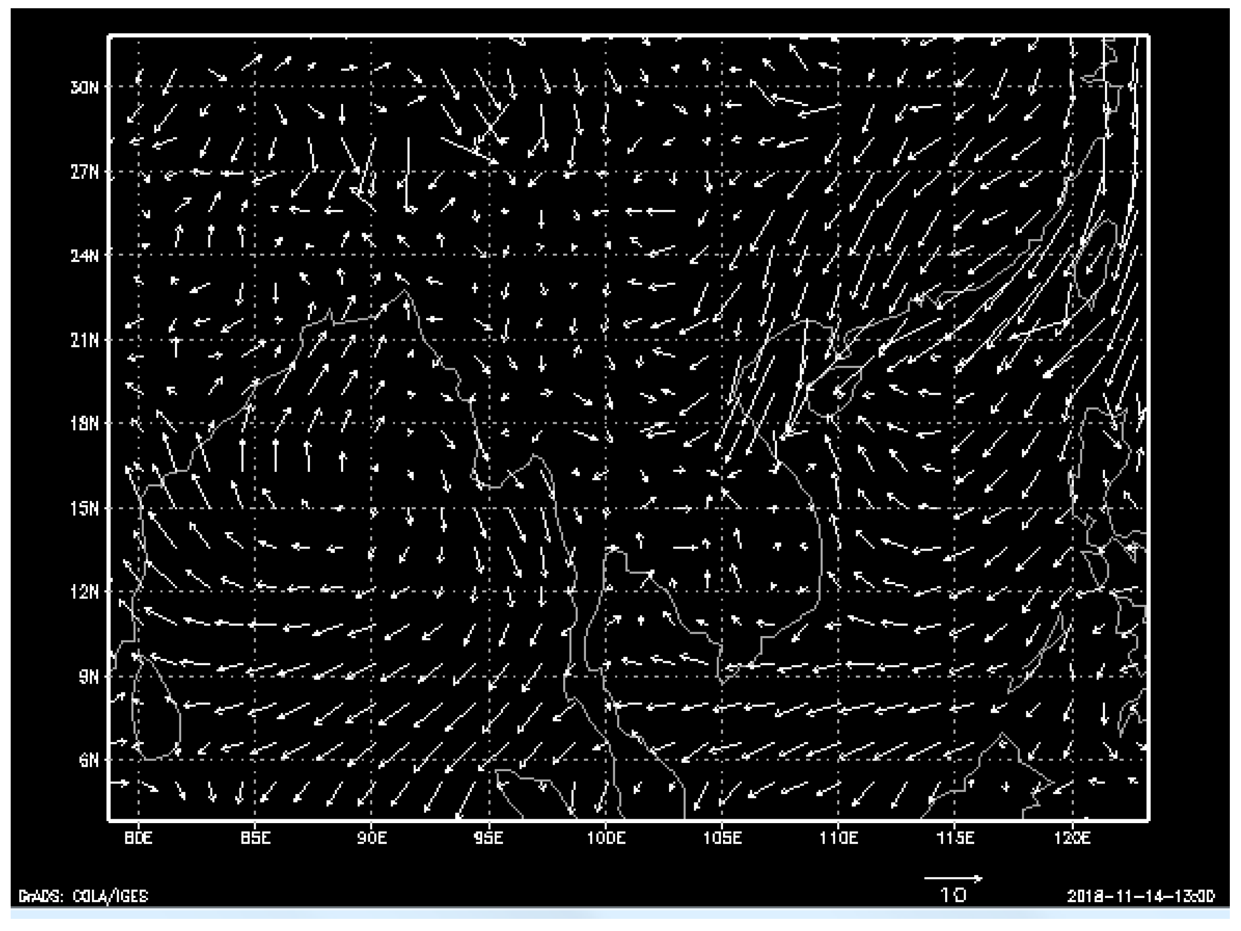
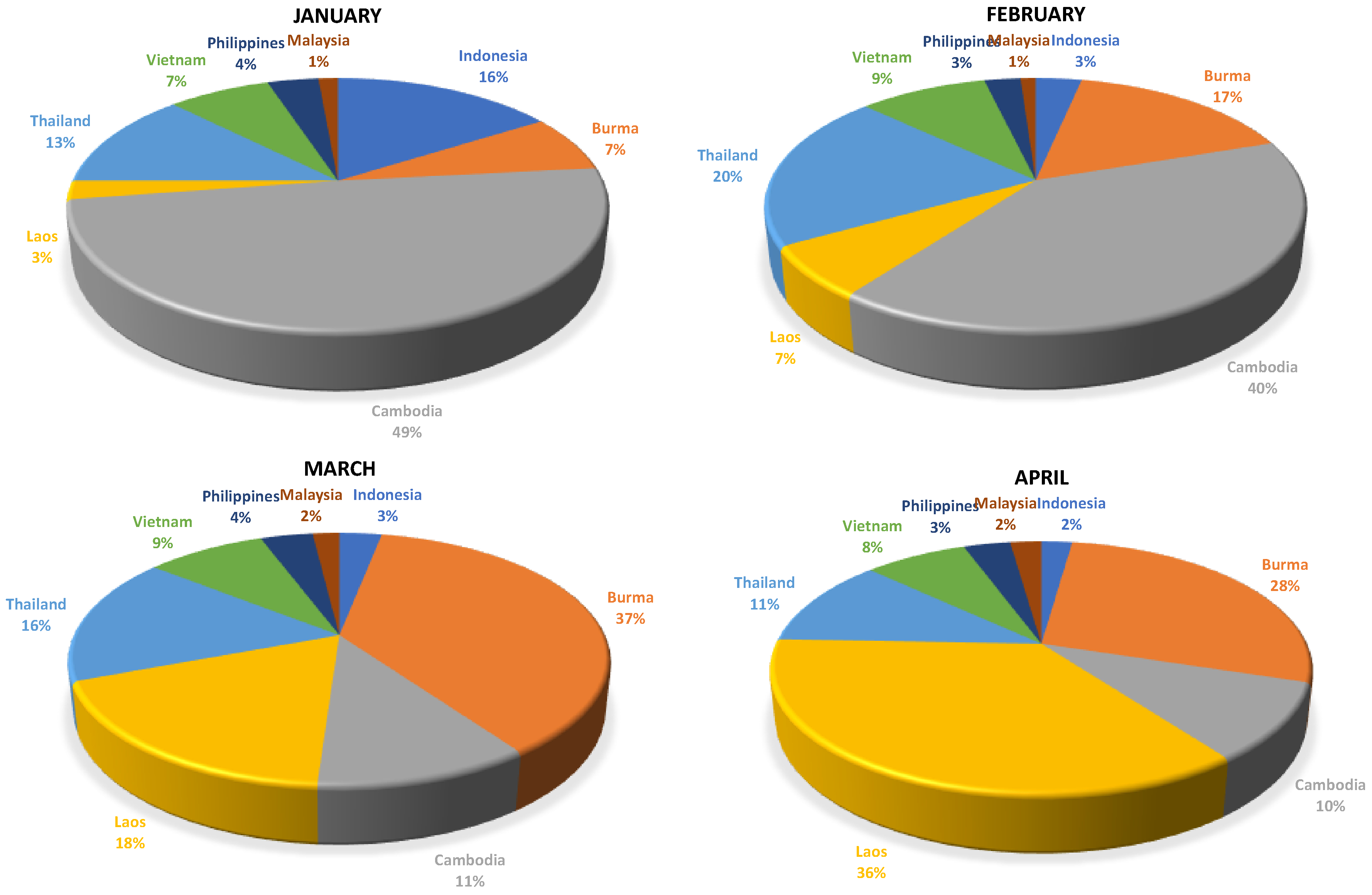
This paper aimed to understand the potential contributions of biomass burning to PM2.5 pollution in Northern Thailand. We developed a coupled atmospheric and air pollution modeling system based on the Weather Research and Forecasting Model and a Hybrid Single-Particle Lagrangian Integrated Trajectory Model (HYSPLIT). The WRF model was used with 1 domain of 20 km grid spacing covering Southeast Asia, some parts of India, and China. The final analysis data were used as a meteorological initial and boundary condition. The model results, including temperature and wind speed, were compared with the ground-based measurements from the Pollution Control Department (PCD) in northern Thailand. The model’s capability was shown to be acceptable when compared to observations, as indicated by the Index of Agreement (IOA) in ranges of 0.57 to 0.79 for temperature and 0.32 to 0.54 for wind speed, while the fractional bias of temperature and wind speed were 1.3 to 2.5 °C and 1.2 to 2.1 m/s. The meteorological and trajectory analysis found that the influence of the Asian Winter Monsoon can carry air pollutants to northern Thailand through two major channels. The first channel is characterized by winds blowing from eastern Asia towards Laos into northern Thailand, while the second channel is characterized by northwesterly winds blowing from Burma and entering northern Thailand. Additionally, the low temperature and wind speed during this time in northern Thailand provide favorable conditions that contribute to the air pollution problem. The analysis of Near Real Time (NRT) Moderate Imaging Spectroradiometer (MODIS) hotspot data indicated that the biomass burning from Burma has greater potential to contribute to the air pollution problem in Thailand compared to national emissions.

References

1. WHO. 7 Million Premature Deaths Annually Linked to Air Pollution. Available online: http://www.who.int/mediacentre/news/releases/2014/air-pollution/en/ (accessed on 11 November 2020).
2. Seinfeld, J.H.; Pandis, S.N. Atmospheric Chemistry and Physics: From Air Pollution to Climate Change; John Wiley & Sons: Hoboken, NJ, USA, 2016. [Google Scholar]
3. Yin, S.; Wang, X.; Zhang, X.; Guo, M.; Miura, M.; Xiao, Y. Influence of biomass burning on local air pollution in mainland Southeast Asia from 2001 to 2016. Environ. Pollut. 2019, 254, 112949. [Google Scholar] [CrossRef] [PubMed]
4. Lee, H.H.; Iraqui, O.; Gu, Y.; Yim, S.H.L.; Chulakadabba, A.; Tonks, A.Y.M.; Yang, Z.; Wang, C. Impacts of air pollutants from fire and non-fire emissions on the regional air quality in Southeast Asia. Atmos. Chem. Phys. 2018, 18, 6141–6156. [Google Scholar] [CrossRef] [Green Version]
5. Lee, H.H.; Iraqui, O.; Wang, C. The Impact of Future Fuel Consumption on Regional Air Quality in Southeast Asia. Sci. Rep. 2019, 9, 2648. [Google Scholar] [CrossRef] [PubMed]
6. Oanh, N.K.; Upadhyay, N.; Zhuang, Y.-H.; Hao, Z.-P.; Murthy, D.; Lestari, P.; Villarin, J.; Chengchua, K.; Co, H.; Dung, N. Particulate air pollution in six Asian cities: Spatial and temporal distributions, and associated sources. Atmos. Environ. 2006, 40, 3367–3380. [Google Scholar] [CrossRef]
7. Oanh, N.T.K.; Leelasakultum, K. Analysis of meteorology and emission in haze episode prevalence over mountain-bounded region for early warning. Sci. Total Environ. 2011, 409, 2261–2271. [Google Scholar] [CrossRef]
8. Amnuaylojaroen, T.; Kreasuwun, J.; Towta, S.; Siriwitayakorn, K. Dispersion of particulate matter (PM10) from forest fires in Chiang Mai province, Thailand. Chiang Mai J. Sci. 2010, 37, 39–47. [Google Scholar]
9. Amnuaylojaroen, T.; Kreasuwun, J. Investigation of fine and coarse particulate matter from burning areas in Chiang Mai, Thailand using the WRF/CALPUFF. Chiang Mai J. Sci. 2012, 39, 311–326. [Google Scholar]
10. Thai Meteorological Department. The Climate of Thailand. Available online: https://www.tmd.go.th/en/archive/thailand_climate.pdf (accessed on 11 November 2020).
11. Cheng, I.; Zhang, L.; Blanchard, P.; Dalziel, J.; Tordon, R. Concentration-weighted trajectory approach to identifying potential sources of speciated atmospheric mercury at an urban coastal site in Nova Scotia, Canada. Atmos. Chem. Phys. 2013, 13, 6031–6048. [Google Scholar] [CrossRef] [Green Version]
12. Amnuaylojaroen, T.; Macantangay, R.C.; Khodmanee, S. Modeling the effect of VOCs from biomass burning emissions on ozone pollution in upper Southeast Asia. Heliyon 2019, 5, e02661. [Google Scholar] [CrossRef] [Green Version]
13. Lelieveld, J.; Barlas, C.; Giannadaki, D.; Pozzer, A. Model calculated global, regional and megacity premature mortality due to air pollution. Atmos. Chem. Phys. 2013, 13, 7023–7037. [Google Scholar] [CrossRef] [Green Version]
14. Vichit-Vadakan, N.; Ostro, B.D.; Chestnut, L.G.; Mills, D.M.; Aekplakorn, W.; Wangwongwatana, S.; Panich, N. Air pollution and respiratory symptoms: Results from three panel studies in Bangkok, Thailand. Environ. Health Perspect. 2001, 109, 381–387. [Google Scholar] [PubMed] [Green Version]
15. Tsai, F.C.; Smith, K.R.; Vichit-Vadakan, N.; Ostro, B.D.; Chestnut, L.G.; Kungskulniti, N. Indoor/outdoor PM10 and PM2.5 in Bangkok, Thailand. J. Expo. Anal. Environ. Epidemiol. 2000, 10, 15–26. [Google Scholar] [CrossRef] [PubMed] [Green Version]
16. Jinsart, W.; Tamura, K.; Loetkamonwit, S.; Thepanondh, S.; Karita, K.; Yano, E. Roadside particulate air pollution in Bangkok. J. Air Waste Manag. Assoc. 2002, 52, 1102–1110. [Google Scholar] [CrossRef] [PubMed] [Green Version]
17. Chueinta, W.; Hopke, P.K.; Paatero, P. Investigation of sources of atmospheric aerosol at urban and suburban residential areas in Thailand by positive matrix factorization. Atmos. Environ. 2000, 34, 3319–3329. [Google Scholar] [CrossRef]
18. Chueinta, W.; Bunprapob, S. Elemental Quantification and Source Identification of Airborne Particulate Matter in Pathumwan District; Chemistry and Material Science Research Program, Office of Atoms for Peace: Bangkok, Thailand, 2003. [Google Scholar]
19. Leenanupan, V.; Harnvong, T.; Sritusnee, U.; Bovornkitti, S. Elemental composition of atmospheric particulates in Mae Hong Son province. J. Health Sci. 2002, 11, 525–533. [Google Scholar]
20. Ebihara, M.; Chung, Y.; Chueinta, W.; Ni, B.-F.; Otoshi, T.; Oura, Y.; Santos, F.; Sasajima, F.; Wood, A. Collaborative monitoring study of airborne particulate matters among seven Asian countries. J. Radioanal. Nucl. Chem. 2006, 269, 259–266. [Google Scholar] [CrossRef]
21. Ebihara, M.; Chung, Y.; Dung, H.; Moon, J.; Ni, B.-F.; Otoshi, T.; Oura, Y.; Santos, F.; Sasajima, F.; Wee, B. Application of NAA to air particulate matter collected at thirteen sampling sites in eight Asian countries: A collaborative study. J. Radioanal. Nucl. Chem. 2008, 278, 463–467. [Google Scholar] [CrossRef]
22. Hopke, P.K.; Cohen, D.D.; Begum, B.A.; Biswas, S.K.; Ni, B.; Pandit, G.G.; Santoso, M.; Chung, Y.-S.; Davy, P.; Markwitz, A. Urban air quality in the Asian region. Sci. Total Environ. 2008, 404, 103–112. [Google Scholar] [CrossRef]
23. NCAR. NCEP FNL Operational Model Global Tropospheric Analyses, Continuing from July 1999. Available online: https://0-doi-org.brum.beds.ac.uk/10.5065/D6M043C6 (accessed on 11 November 2020).
24. Skamarock, W.; Klemp, J.B.; Dudhia, J.; Gill, D.O.; Barker, D.; Duda, M.G.; Huang, X.-Y.; Wang, W. A Description of the Advanced Research WRF Version 3. NCAR Technical Note NCAR/TN-475+STR; University Corporation for Atmospheric Research: Boulder, CO, USA, 2008. [Google Scholar] [CrossRef]
25. Hong, S.-Y.; Dudhia, J.; Chen, S.-H. A revised approach to ice microphysical processes for the bulk parameterization of clouds and precipitation. Mon. Weather Rev. 2004, 132, 103–120. [Google Scholar] [CrossRef]
26. Hong, S.-Y.; Lim, J.-O.J. The WRF single-moment 6-class microphysics scheme (WSM6). Asia Pac. J. Atmos. Sci. 2006, 42, 129–151. [Google Scholar]
27. Kain, J.S. The Kain–Fritsch convective parameterization: An update. J. Appl. Meteorol. 2004, 43, 170–181. [Google Scholar] [CrossRef] [Green Version]
28. Paulson, C.A. The mathematical representation of wind speed and temperature profiles in the unstable atmospheric surface layer. J. Appl. Meteorol. 1970, 9, 857–861. [Google Scholar] [CrossRef]
29. Dyer, A.; Hicks, B. Flux-gradient relationships in the constant flux layer. Q. J. R. Meteorol. Soc. 1970, 96, 715–721. [Google Scholar] [CrossRef]
30. Webb, E.K. Profile relationships: The log-linear range, and extension to strong stability. Q. J. R. Meteorol. Soc. 1970, 96, 67–90. [Google Scholar] [CrossRef]
31. Beljaars, A.C. The parametrization of surface fluxes in large-scale models under free convection. Q. J. R. Meteorol. Soc. 1995, 121, 255–270. [Google Scholar] [CrossRef]
32. Zhang, D.; Anthes, R.A. A high-resolution model of the planetary boundary layer—Sensitivity tests and comparisons with SESAME-79 data. J. Appl. Meteorol. 1982, 21, 1594–1609. [Google Scholar] [CrossRef]
33. Draxler, R.R.; Hess, G.D. An overview of the HYSPLIT_4 modelling system for trajectories. Aust. Meteorol. Mag. 1998, 47, 295–308. [Google Scholar]
34. Kantha, L.H.; Clayson, C.A. Small scale processes in geophysical fluid flows. Int. Geophys. Ser. 2000, 68, 883. [Google Scholar]
35. Wurps, H.; Steinfeld, G.; Heinz, S. Grid-Resolution Requirements for Large-Eddy Simulations of the Atmospheric Boundary Layer. Bound. Layer Meteorol. 2020, 175, 1–23. [Google Scholar] [CrossRef] [Green Version]
36. Jones, A.M.; Harrison, R.M.; Baker, J. The wind speed dependence of the concentrations of airborne particulate matter and NOx. Atmos. Environ. 2010, 44, 1682–1690. [Google Scholar] [CrossRef]
37. Giglio, L.; Schroeder, W.; Justice, C.O. The collection 6 MODIS active fire detection algorithm and fire products. Remote Sens. Environ. 2016, 178, 31–41. [Google Scholar] [CrossRef] [PubMed] [Green Version]
Figure 1. Domain configuration.
Sustainability 12 10049 g001
Figure 2. Average wind speed and temperature between the 1-h WRF model output (gray) and the hourly observations from PCD (yellow), as well as the 24-h WRF model output (orange-dots) and the 24-h observation from PCD (blue-dots).
Sustainability 12 10049 g002aSustainability 12 10049 g002b
Figure 3. Average wind speed and direction from the WRF model in March 2016.
Sustainability 12 10049 g003
Figure 4. Relationship between temperature and PM2.5 (up), wind speed, and PM2.5 (low).
Sustainability 12 10049 g004
Figure 5. Hybrid Single-Particle Lagrangian Integrated Trajectory (HYSPLIT) backward ensemble Table (a) 500. m, (b) 1000 m, and (c) 1500 m, beginning on 0000 UTC 20 March 2016 and ending on 0000 UTC 27 March 2016 in northern Thailand.
Sustainability 12 10049 g005
Figure 6. HYSPLIT backward ensemble trajectories initiated at (a) 2000 m, (b) 2500 m, and (c) 3000 m, beginning on 0000 UTC 20 March 2016 and ending on 0000 UTC 27 March 2016 in northern Thailand.
Sustainability 12 10049 g006
Figure 7. The proportion of hotspot locations for each country in Southeast Asia.
Sustainability 12 10049 g007
Figure 8. Monthly and daily PM2.5 concentrations in March 2016 in northern Thailand.
Sustainability 12 10049 g008