The Effect of Willow (Salix sp.) on Soil Moisture and Matric Suction at a Slope Scale


The BEAM Research Centre, School of Computing, Engineering and Built Environment, Glasgow Caledonian University, Glasgow G4 0BA, UK
*
Author to whom correspondence should be addressed.
Sustainability 2020, 12(23), 9789; https://0-doi-org.brum.beds.ac.uk/10.3390/su12239789
Submission received: 4 September 2020
/
Revised: 18 November 2020
/
Accepted: 19 November 2020
/
Published: 24 November 2020
(This article belongs to the Special Issue Sustainable Use of Nature-Based Solutions for Erosion Control and Slope Protection)
Abstract
:The aim of this study is to provide new knowledge on the effect of willow on hillslope hydrology at a slope scale. Soil moisture and matric suction were monitored in situ under willow-vegetated and fallow ground covers on a small-scale hillslope in Northeast Scotland for 21 months. The retrieved time series were analysed statistically to evaluate whether the dynamics of soil moisture and matric suction changed with the hillslope zone (i.e., toe, middle, and crest) under the two ground covers. The effect of air temperature and rainfall on the dynamics of soil moisture and matric suction, as well as the relationship between the two soil-water variables, under both ground covers, were also investigated by analysing the cross-correlation between time series. The results of 21 months of monitoring showed that willow contributed substantially to reduce soil moisture and to increase matric suction with respect to fallow soil. Additionally, willow-vegetated soil exhibited higher water retention and moisture buffering capacity than fallow soil. The effect of willow was highest at the hillslope toe due to a denser vegetation cover present within this zone. Both air temperature and rainfall had a strong effect on soil moisture and matric suction. However, the effect of air temperature was more consistent and easier to interpret than that of rainfall. Soil moisture and matric suction were shown to have a complex relationship and the soil water characteristic curve for vegetated soil requires further research. This study provides novel, field-based information supporting the positive effect of willow on hillslope hydrology. The results gathered herein will undoubtedly enhance the confidence of using woody vegetation in Nature-based Solutions (NBS) against geo-climatic hazards.
1. Introduction
Vegetation can effectively provide mechanical and hydrological stability to soil-mantled hillslopes [1]. On the one hand, vegetation roots can mechanically reinforce the soil by adding cohesion and structural strength [2]. On the other, vegetation can contribute to regulate the hydrological cycle in the soil by intercepting and funnelling rainfall above the ground [3], by encouraging drainage and preferential flow below the ground [4], by withdrawing soil water through plant uptake and evapotranspiration [3], or by changing the behaviour of soil-water dynamics [5]. The acknowledged ability of vegetation to reinforce the soil mechanically and hydrologically has encouraged the use of living plant materials in Nature-based Solutions (NBS; [6]) and eco-engineering, or ground bio-engineering, strategies against hydro-meteorological and geo-hydrological hazards worldwide [7,8,9]. While the hydrological effects of different species have been investigated, usually separately, in the past, the hydrological contribution of vegetation to slope reinforcement has seldom been quantified at a slope scale.
The study of hillslope hydrology has been topical over recent decades (e.g., [10,11,12]) due to its relationship with natural phenomena such as runoff, river discharge, flooding, or soil erosion. Understanding the relationship between hillslope hydrology and soil mechanics has gained relevance over the last ten years (e.g., [11]) as rainfall-induced landslides are becoming more ubiquitous, frequent, and severe as a result of climate change [13]. The knowledge on how hillslope hydrology changes spatially along hillslope transects is still poor (e.g., [14,15,16]) but, generally, researchers agree that water tends to flow and accumulate towards the toe of a hillslope [11]. Similarly, there is generally a good understanding on how soil water affects the mechanical strength of slope-forming materials (e.g., [17,18]). In this regard, the relationship between the soil moisture and matric suction established through the soil water characteristic curve (SWCC; [19]) provides a good basis to bridge soil hydrology and mechanics [18]. Still, SWCCs for plant–soil composites either are difficult to obtain or have not yet been reported accurately (e.g., [3,20,21]). Moreover, only a handful of field studies have been undertaken to collect field-based knowledge on how vegetation influences the distribution of soil moisture and matric suction within hillslopes (e.g., [3,16,22]).
The investigation of the effect of vegetation on hillslope hydrology is labour-intensive and methodologically challenging. It also requires effective implementation of multidisciplinary approaches to understand the complex processes occurring at the plant–soil–atmosphere interface [23]. These processes are mostly described through readily measurable meteorological variables such as air temperature and rainfall [24], as both are tightly coupled with the hydrological cycle in the soil [25] and modulate the atmospheric demand for water [26]. However, and to the best of our knowledge, there is no convincing information on how temperature and rainfall shape the effect of vegetation on hillslope hydrology [4], as of yet, perhaps due to the lack of reliable time series measurements of these parameters. Gaining insight into how the readily available meteorological variables drive complex processes at the plant–soil–atmosphere continuum would open up an opportunity to establish reliable indicators for the hydrological performance of vegetation in NBS and eco-engineering projects [27].
Willow (Salix sp.) is a pioneer plant species, very often used in NBS and eco-engineering projects. The genus Salix comprises over 400 species of deciduous shrubs and trees that primarily grow on moist soils in cold and temperate regions of the Northern Hemisphere [28]. Willow is readily propagated from branches and cuttings, grows quickly in temperate climates, and it can thrive in water-logged environments and contaminated soil [29]. Willow cuttings and fascines are commonly used as complementary construction materials in NBS such as cribwalls, palisades, slope gratings, or brush layers [7]. Willow can facilitate a quick establishment of dense vegetation covers and provide additional and long-lasting strength to engineering interventions seeking to provide stability and protection in riverbanks and hillslopes [30,31]. Understanding the effect of willow as a basic, pioneer vegetation on hillslope hydrology is, therefore, crucial to ensure the success of NBS and eco-engineering strategies. In the past, the mechanical effects of willow on soil reinforcement have been studied (e.g., [32]) more than the hydrological (e.g., [3]), although never in combination at a stand or slope scale.
The aim of this study was to provide new knowledge on the effect of willow on hillslope hydrology, through in situ monitoring of soil moisture and matric suction under willow-vegetated and fallow ground covers on a small-scale hillslope in Northeast Scotland. The specific objectives of this study were to:
- (i)
- Assess the differences between willow-vegetated and fallow ground covers in terms of soil moisture and matric suction.
- (ii)
- Evaluate whether the dynamics of soil moisture and matric suction changed with the hillslope zone (i.e., toe, middle, and crest) under the different ground covers.
- (iii)
- Investigate the relationship between the soil moisture and matric suction at different hillslope zones under both ground covers.
- (iv)
- Investigate the effect of air temperature and rainfall on the dynamics of soil moisture and matric suction under both ground covers.
2. Materials and Methods
2.1. Study Site
The study site is located in Catterline Bay, Aberdeenshire, UK (WGS84 Long: −2.21 Lat: 56.90). The climate is temperate humid (Cgc: subpolar oceanic climate; [33]). The mean annual temperature of the site over the period 2011–2018 was 8.9 °C and the mean annual rainfall was 556.8 mm. Precipitation is in the form of frequent, low-intensity rainfall events and the prevailing wind is south-westerly.
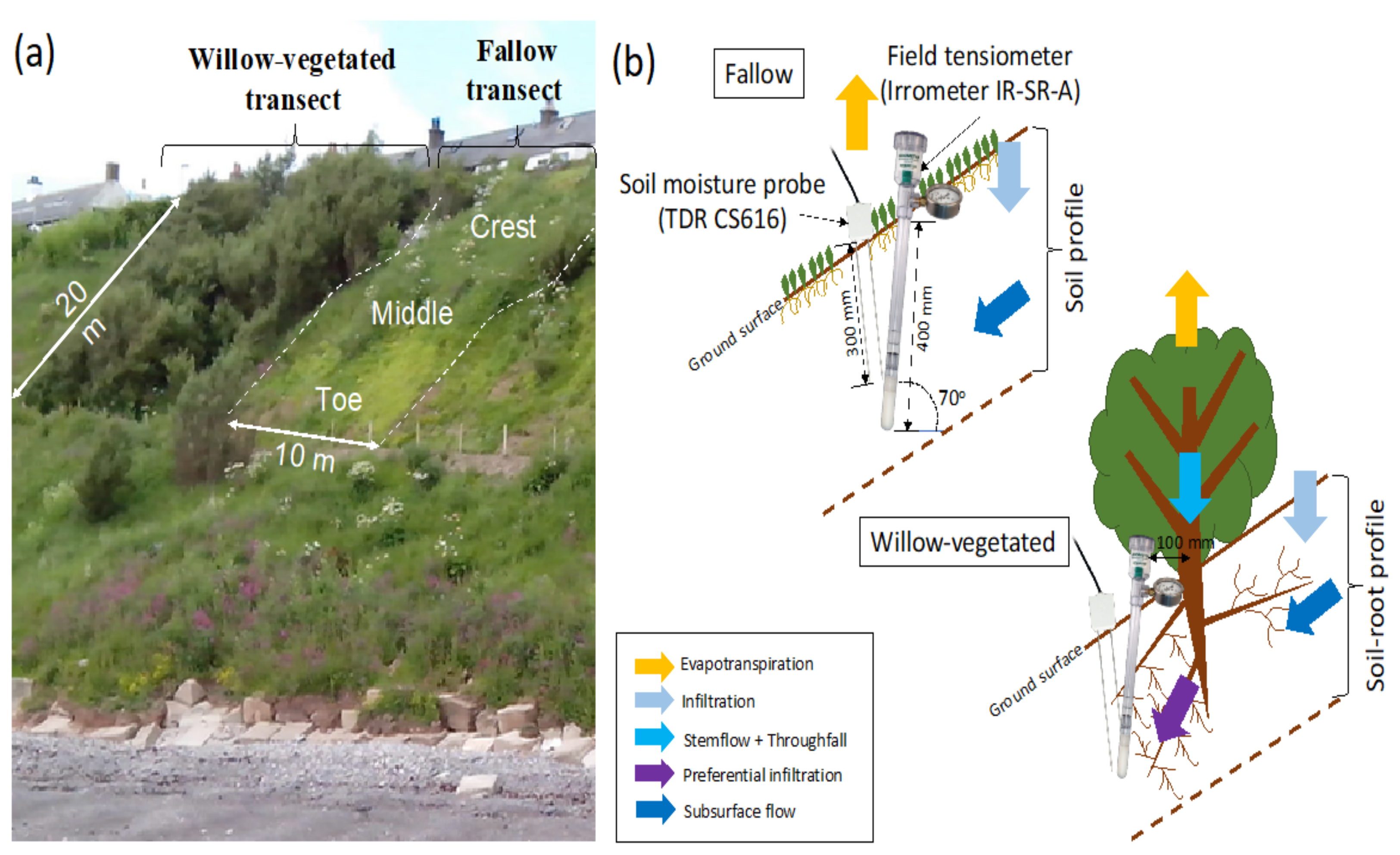
Two adjacent 10 × 20 m hillslope transects with a similar mean slope gradient (25.6°) were chosen to study the effect of willow on hillslope hydrology (Figure 1a). The vegetated transect, originally planted in the early 1990s, included a dense mixture of 30 year-old willow belonging to two different, albeit eco-physiologically similar, species—i.e., basket willow (Salix viminalis L.; mostly distributed near the toe of the slope; approx. 30% of the transect area), and goat willow (Salix caprea L.; mostly distributed in the middle and crest zones of the slope; approx. 70% of the transect area). The vegetation cover was denser (i.e., >2 willow stems m−2) at the toe of the hillslope compared to the upper parts of the slope (i.e., <1 willow stem m−2). The aboveground traits of the monitored willow individuals are shown in Table 1. The other transect (i.e., fallow transect) had a sparse vegetation cover mainly comprising pioneer grasses and herbs [34].
Shallow (<1000 mm deep) and organic matter-rich (SOM = 5.6%) silty sand soil underlies the two studied transects (gravel: 11.2%; sand: 79.8%; silt: 5.9%; clay: 3.1%), with mean dry bulk density (ρb) of 1.1 and 0.7 g cm−3 for the fallow and willow-vegetated transect, respectively, a saturated hydraulic conductivity (Ks) of 5.82 × 10⁻⁵ m s−1, a drained cohesion of 33.4 kPa, and a mean angle of internal friction of 22° [1,2].
2.2. Experimental Setup
In early 2015, the willow-vegetated and fallow hillslope transects were instrumented with already calibrated automatic probes measuring the volumetric soil moisture content (θv; %) and the soil matric suction (φ; kPa) (Figure 1b). The volumetric soil moisture was measured with six time-domain reflectometry sensors (TDR; CS616—Campbell Scientific, UK). Three TDRs were deployed in each hillslope transect at the toe, middle, and crest zone, respectively. In the fallow transect, each TDR sensor was vertically inserted in the ground, monitoring θv between 0 and 300 mm below the ground level (b.g.l; Figure 1b). In the willow-vegetated transect, the three TDR sensors were installed vertically and adjacent to three representative adult willow individuals and 100 mm away from the stem in the downslope direction (Figure 1b), monitoring θv between 0 and 300 mm b.g.l within the rooting zone. The soil matric suction was measured with six tensiometers (IR-SR-A—Irrometer, USA) consisting of an automatic pressure gauge and a 450 mm long shaft filled with de-aired, de-ionised water. The tensiometers were deployed in 400 mm deep boreholes made with a soil core auger. Each tensiometer was inserted in the borehole at an angle of ca. 70° with the horizontal (Figure 1b). Each tensiometer was installed adjacent to a TDR and the soil around the installations was allowed to settle before the first measurement. All sensors were wired to a solar-powered CR-1000 data logger (Campbell Scientific, UK). A 5-Volt, voltage regulator was used to supply power to the tensiometers and the following calibration equation was used to convert voltage (V; Volts) into φ (kPa): φ = (4.3 − V)/0.02. Records of θv and φ were logged at 5 min time steps for 21 months.
The two studied soil-water variables (i.e., θv and φ) were compared against two meteorological variables: air temperature (Ta; °C) and rainfall (Pg; mm). Air temperature was included in the study to investigate soil-water dynamics under drying conditions (i.e., in the absence of precipitation), as Ta and soil-water tend to be tightly coupled (e.g., [25]). Rainfall was included in the study to investigate the soil-water dynamics under wetting conditions, and because rainfall is the main input of soil water in the study site. Both meteorological variables were retrieved with a 1-min resolution from a Davis Vantage Pro 2 meteorological station located in situ [35].
2.3. Data Analysis
The retrieved time series for θv, φ, Ta, and Pg were aggregated into mean daily time steps. The resulting daily time series were plotted to visually assess the differences between the willow-vegetated and fallow hillslope transects as well as the zones within the transect—i.e., toe, middle, and crest. The input of missing values in the time series was carried out using two data interpolation methods—the choice between the methods depending on the relative occurrence of missing records within the time series—linear interpolation and ARIMA (i.e., autoregressive integrated moving average) model-based interpolation of the 5-min series. Linear interpolation was only implemented when the missing records were within the time series, while ARIMA model-based interpolation was carried out in all cases in which missing values were found for comparison purposes. To this end, ARIMA model parameters (i.e., p = autoregressive parameter; d = differencing parameter; q = moving average parameter) were selected by interpreting the partial correlogram of each time series [36]. The acceptance or rejection of the fitted ARIMA models was assessed through residuals autocorrelation testing using the Ljung–Box test [37] at the 95% and 99% confidence levels. Eventually, the unknown or missing values for a given time series were predicted through Kalman filtering [38]).
Further θv and φ differences between the two hillslope transects and between the three zones, respectively, were assessed by plotting the probability (PDF) and cumulative (CDF) distribution functions. Statistically significant differences in terms of θv and φ, respectively, between the two hillslope transects and between the three zones within each transect were evaluated with the Kolmogorov–Smirnov test (K–S) at the 95% and 99% confidence levels. The K–S index (D) retrieved from performing K–S tests quantifies whether the distance between two CDFs is statistically significant [39]). Hence, D was regarded herein as an indicator of how different the two time series were.
The stationarity of the daily time series was checked with the Dickey–Fuller test (D–F; [36]) at the 95% and 99% confidence levels, and supplemented with the visual examination of the autocorrelogram and partial autocorrelogram plots. The cross-correlation of the soil moisture and matric suction time series with air temperature and rainfall was investigated to highlight any relationship between the two investigated soil-water and meteorological variables. In addition, the cross-correlation between soil moisture and matric suction was examined to shed light on the relationship between the two studied soil hydrological variables over time under fallow and vegetated ground conditions, respectively.
All data analyses and statistical testing were undertaken in the statistical computing software R v3.5.1 [40].
3. Results
3.1. Soil Moisture
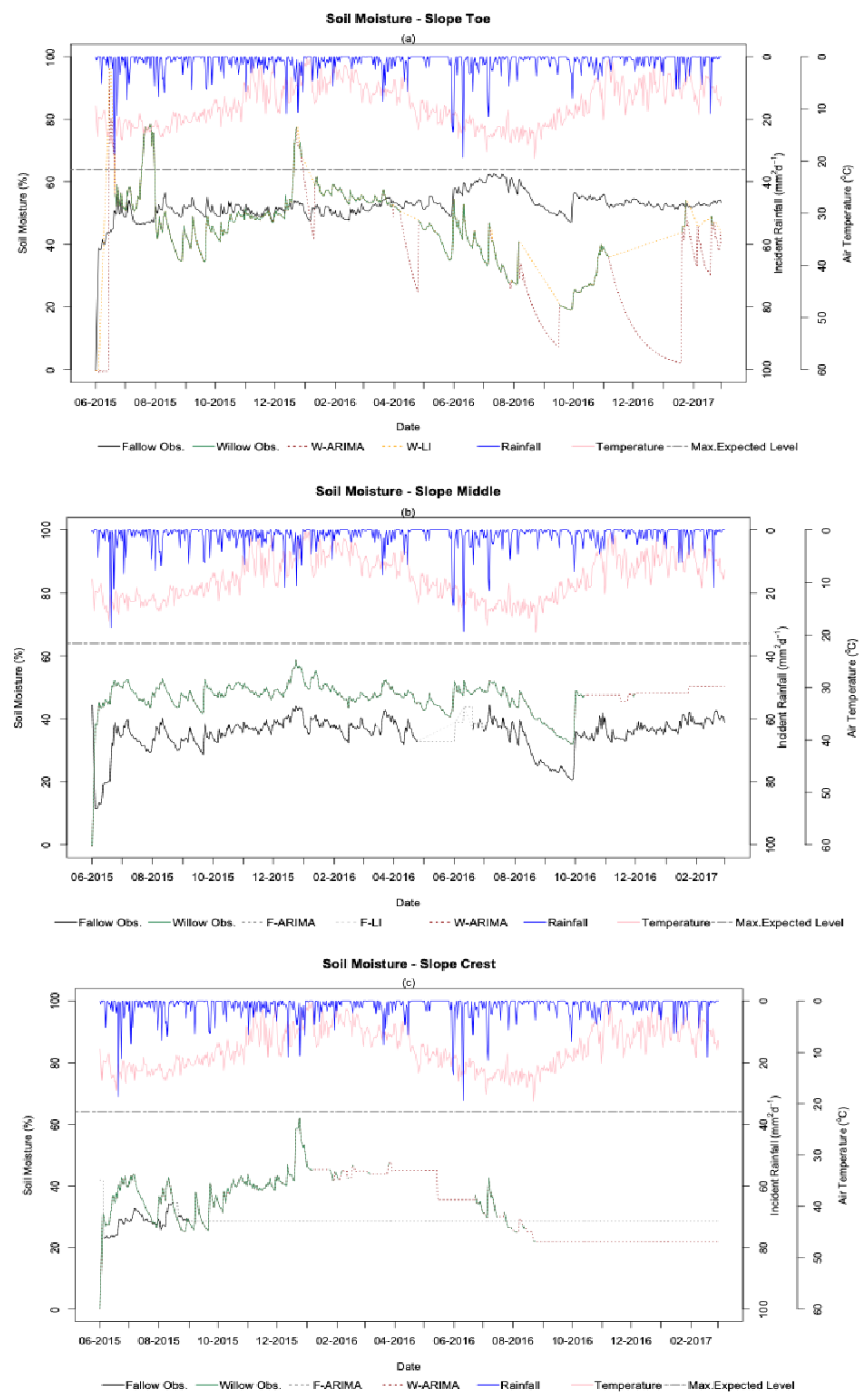
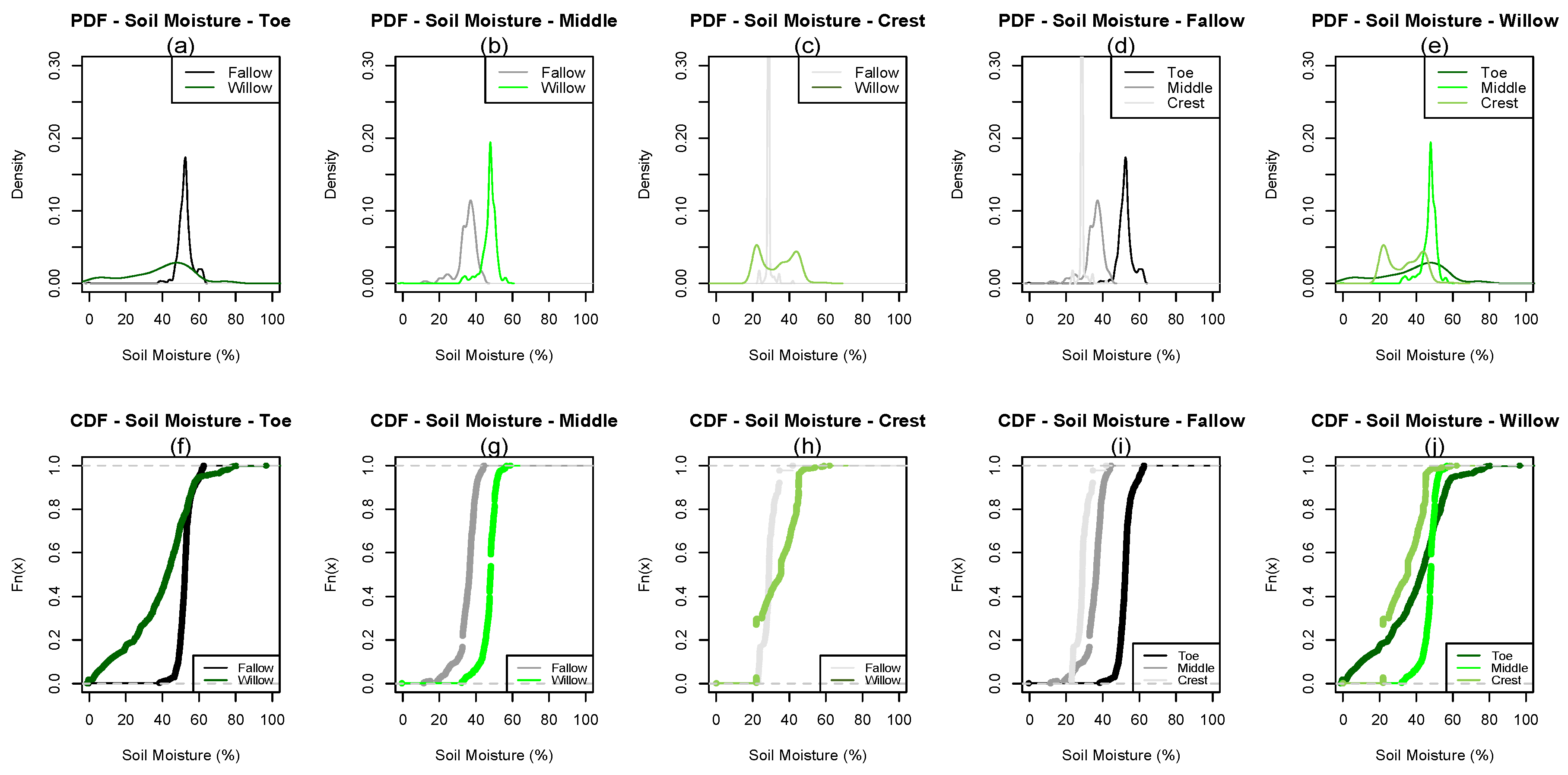
The daily soil volumetric moisture content (θv; Figure 2a–c and Figure 3a–j) showed clear differences between the transects and between the hillslope zones within each transect. The highest recorded θv of 77.6% was found at the toe zone in the willow-vegetated transect in August 2015. The lowest recorded θv of +11.4% was found at the middle zone in the fallow transect in June 2015. A positive response of θv to daily rainfall (Pg) was generally noticed in the time series plots (Figure 2a–c)—i.e., higher Pg led to higher θv, as well as a negative response of θv to mean daily air temperature (Ta)—i.e., higher Ta led to lower θv. At the toe of the slope, θv was statistically significantly higher (D = 0.58 p < 0.01) in the fallow than in the willow-vegetated transect (Figure 3a,f). However, θv differences between the fallow and willow-vegetated transects showed seasonal shifts (Figure 2a). In general, θv was lower in the willow-vegetated than in the fallow transect during the growing season (i.e., May to October) but higher during the dormant season (i.e., November to April). Moreover, and on the basis of the PDFs (Figure 3a,f), the range of observed θv had a greater spread in the willow-vegetated than in the fallow transect. At mid-slope, θv was significantly higher (D = 0.87 p < 0.01) in the willow-vegetated than in the fallow transect (Figure 2b and Figure 3b,g). Soil moisture differences between transects at mid-slope were consistent throughout the observation period (Figure 2b). Additionally, the θv time series followed a similar pattern under fallow and willow-vegetated conditions—i.e., θv increased following rainfall events and θv decreased following periods without rainfall (Figure 2b). At the hillslope crest, a limited amount of θv records were available in both fallow and willow-vegetated transects (Figure 2c) as a result of the TDRs being dysfunctional at this hillslope zone. Nonetheless, during the period of time in which θv records were available, θv was significantly higher (D = 0.49 p < 0.01) in the willow-vegetated than in the fallow transect. Moreover, and on the basis of the PDFs (Figure 3c,h), the range of observed θv had a greater spread in the willow-vegetated than in the fallow transect. Additionally, the PDF for the willow-vegetated transect was bimodal (Figure 3c) as a result of the seasonal θv fluctuations observed in the time series (Figure 2c).
The θv time series were strongly autocorrelated (Supplementary Materials—Figure S1a–f). However, the Augmented Dickey–Fuller test suggested that the θv time series were stationary (i.e., p < 0.01) at the crest and mid-slope of the fallow transect, and at the toe in the willow-vegetated transect. On the basis of the Augmented Dickey–Fuller test, the θv time series were non-stationary (i.e., p > 0.01) at the toe in the fallow transect and at the mid-slope and crest in the willow-vegetated transect.
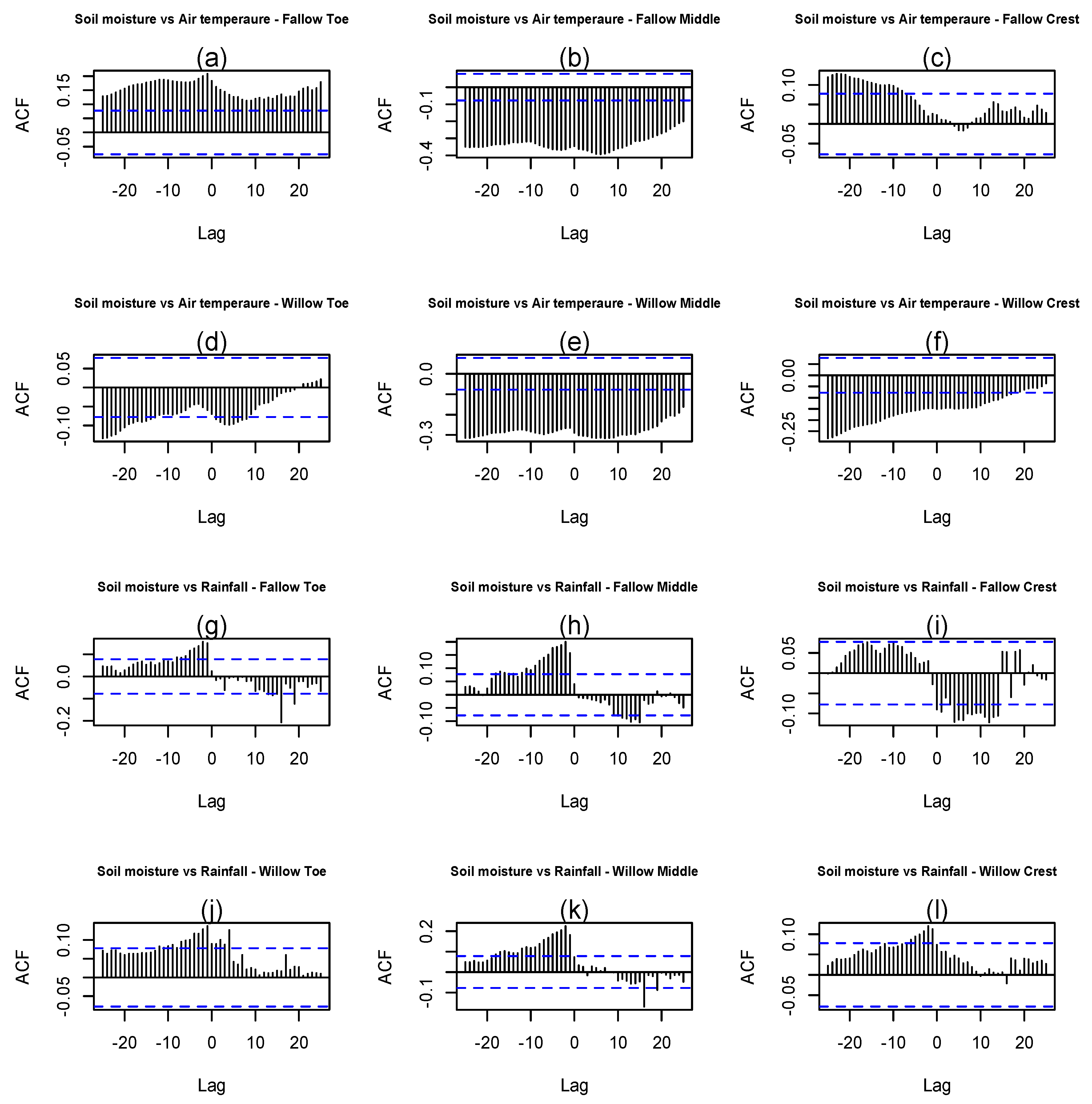
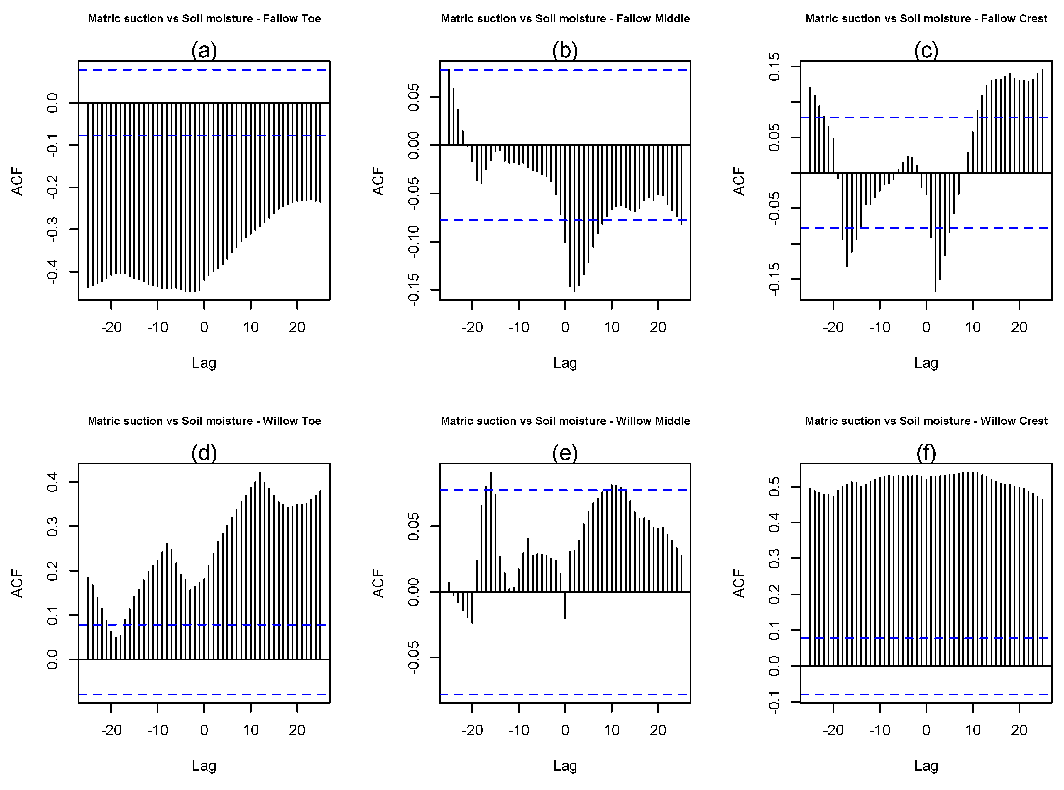
The θv time series were strongly cross-correlated with daily air temperature (Ta; Figure 4a–f) and with daily rainfall (Pg; Figure 4g–l). On the one hand, the cross-correlation between θv and Ta was generally negative (i.e., higher Ta led to lower θv), but positive cross-correlations were observed at the toe and crest in the fallow transect (Figure 4a,c). However, the cross-correlation was only significant at a lag of −7 days (i.e., 7 days before the observation) at the crest of the fallow transect (Figure 4c). On the other hand, the cross-correlation of θv with Pg generally followed a cyclical pattern (Figure 4g–l). Pg and θv were positively cross-correlated before observation (i.e., higher Pg led to higher θv) and negatively cross-correlated after the observation in the fallow transect. Nonetheless, the cross-correlation between Pg and θv was not significant beyond observation in the willow-vegetated transect at the mid-slope and crest (Figure 4k,l), and it remained significantly positive up to a lag of 4 days at the toe of the slope (Figure 4j).
With regard to the input of missing records in the θv time series (Table 2; Figure 2), both linear and ARIMA-based interpolations led to straight line, low-noise interpolations (Figure 2a–c). Linear interpolation was implemented for the mid-slope and toe of the fallow and willow-vegetated transect, respectively. In the fallow transect, the θv time series for the toe zone did not have missing records, whilst the θv time series for the crest were incomplete (Table 2 and Figure 2).
3.2. Matric Suction
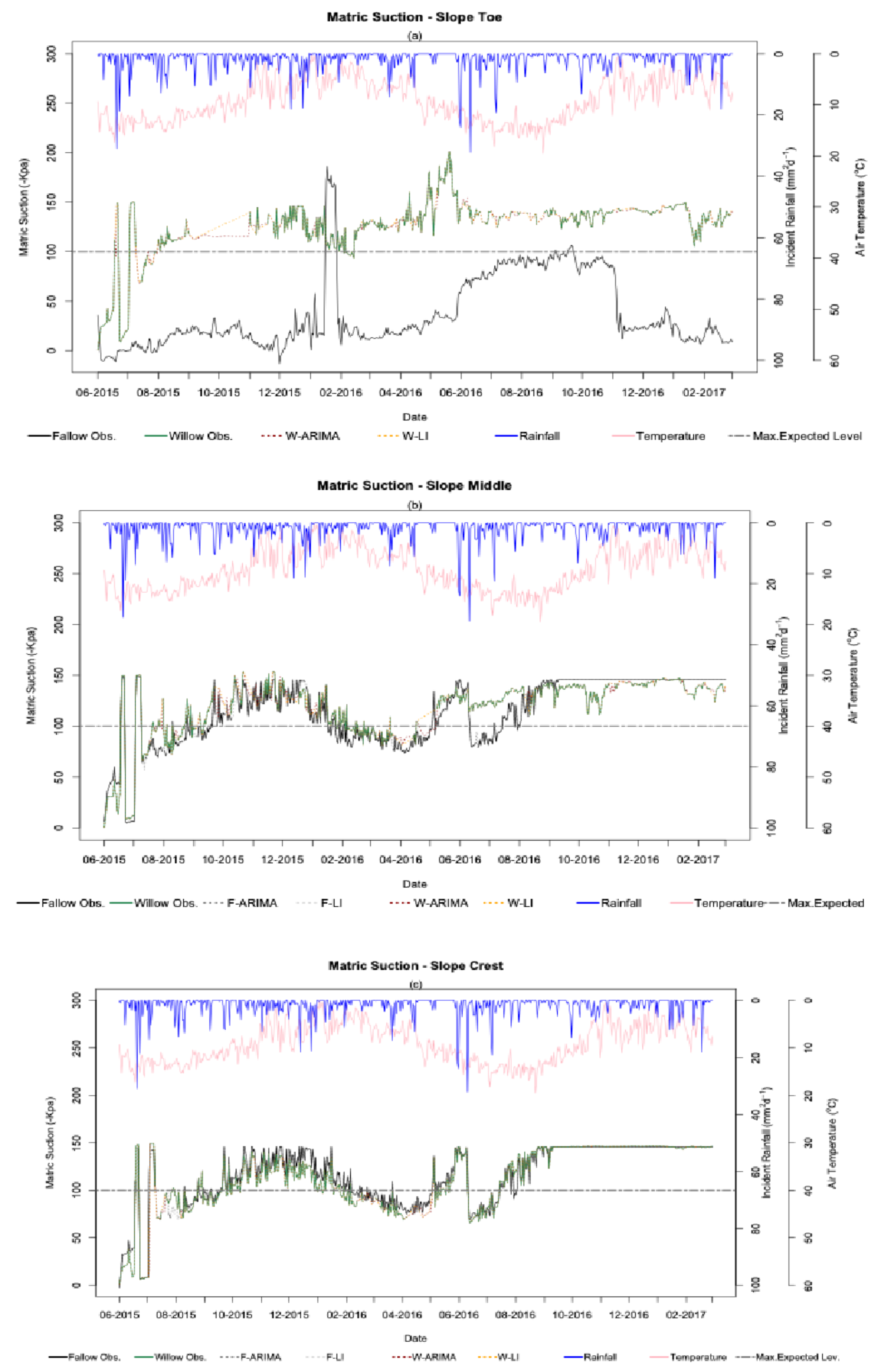
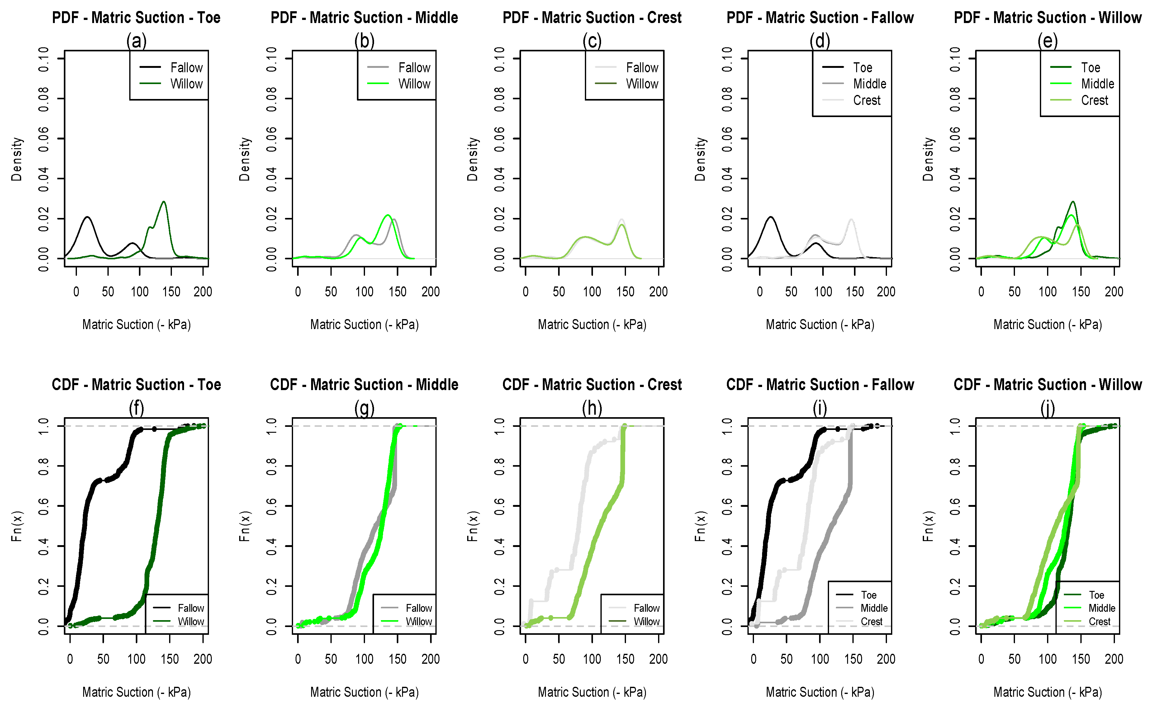
The daily matric suction (φ) showed clear differences between the fallow and willow-vegetated hillslope transects (Figure 5a–c and Figure 6a–j). The highest recorded φ of −201.2 kPa was found at the toe zone in the willow-vegetated transect in May 2016. The lowest recorded φ of +13.6 kPa was found at the toe zone in the fallow transect in December 2015. A negative response of φ to daily rainfall (Pg) was generally observed in the time series plots (Figure 5a–c)—i.e., higher Pg led to lower φ, as well as positive response of φ to mean daily air temperature (Ta)—i.e., higher Ta led to higher φ. Matric suction was significantly higher in the willow-vegetated than in the fallow transect in the three hillslope zones (toe: D = 0.88 p < 0.01; middle: D = 0.24 p < 0.01; crest: D = 0.18 p < 0.01; Figure 6a–j). φ differences between the fallow and willow-vegetated transects were consistent within the toe zone throughout the observation period (Figure 5a), while in the other hillslope zones, they showed some inconsistencies (Figure 5b,c). In the fallow transect, φ differed substantially between the three hillslope zones (D = 0.71 p < 0.01): the highest values measured at the mid-slope and the lowest at the toe (Figure 6i). Moreover, positive pore-water pressures (positive φ records; Figure 5a) were recorded at the toe in the fallow transect. By contrast, the φ differences between the hillslope positions in the willow-vegetated transect (Figure 6j) were not as substantial as in the fallow transect (Figure 6i), where φ was generally higher at the toe when compared to the other two hillslope zones (Figure 6j; D = 0.27 p < 0.01). Linear φ signals were recorded at the mid-slope and crest following the 2016 growing season (Figure 5b,c) as a result of the tensiometers being dysfunctional at these locations. The PDFs for φ (Figure 6a–e) showed that the density distribution of φ was bimodal in all cases except at the toe in the willow-vegetated transect (Figure 6a).
The φ time series were strongly autocorrelated (Supplementary Materials—Figure S1g–l). However, the Augmented Dickey–Fuller test suggested that the φ time series were stationary (i.e., p < 0.01) at all hillslope zones in both fallow and willow-vegetated transects with the exception of the toe zone in the fallow transect, where the time series were non-stationary (D–F = −3.6 p = 0.04).
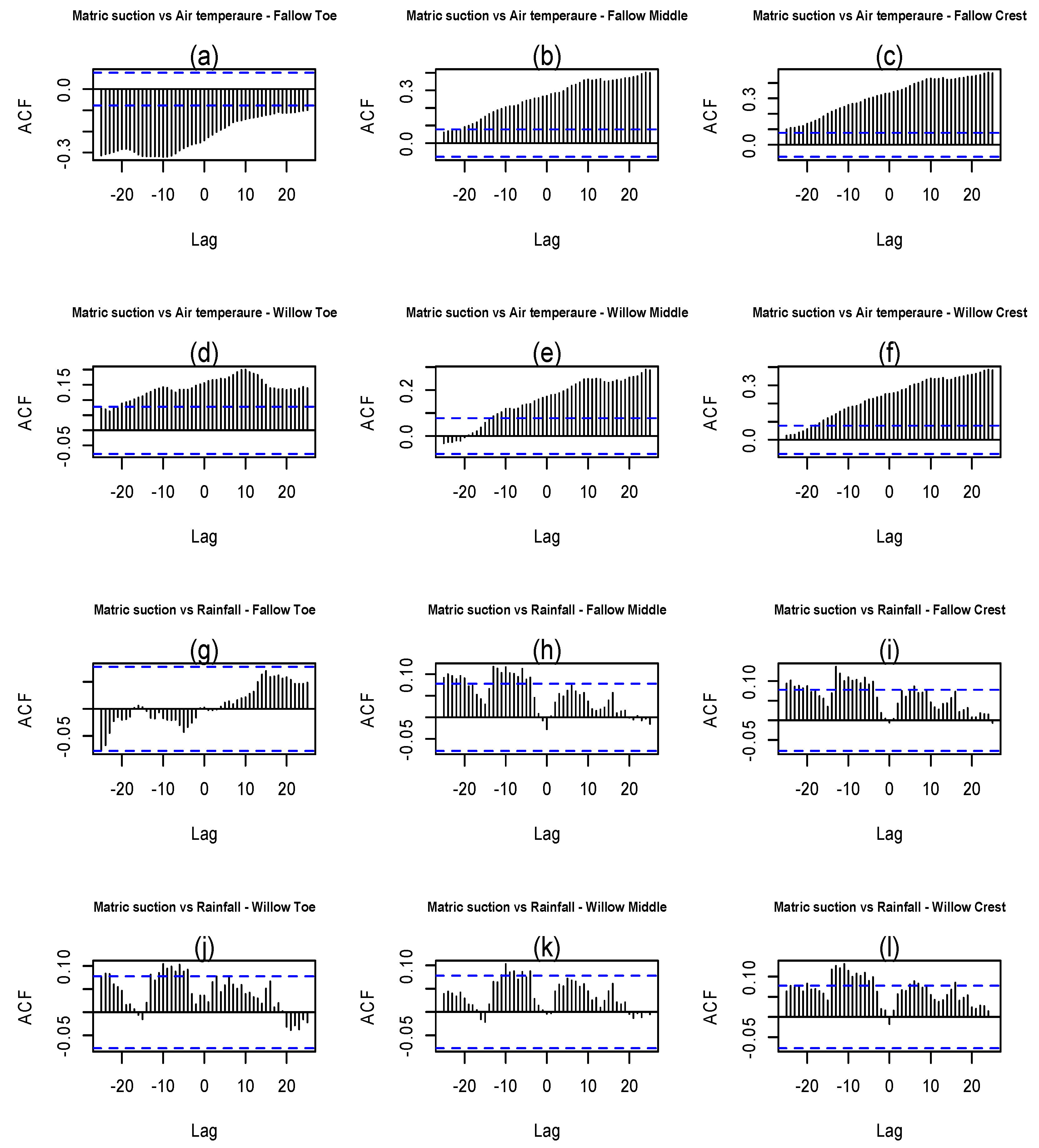
The φ time series were strongly cross-correlated with Ta (Figure 7a–f) and with Pg in most cases (Figure 7g–l). On the one hand, cross-correlation between φ and Ta was generally positive—i.e., higher Ta led to higher φ, despite the strong, negative cross-correlation observed at the toe zone in the fallow transect (Figure 7a). On the other hand, the cross-correlation of φ with Pg was positive and significant at time lags of 4 and 5 days before the observation (Figure 7h–l). However, most φ time series presented a negative, albeit non-significant, cross-correlation with Pg upon observation (Figure 7h,i,k,l). Only the φ time series recorded at the toe zone in the fallow transect showed a shift from negative to positive cross-correlation with Pg before and after observation, although the cross-correlation was not statistically significant at this location (Figure 7a).
With regard to the input of missing records in the φ time series (Table 2; Figure 5), both linear and ARIMA-based interpolation were implemented in all cases for the fallow and willow-vegetated transects. The φ time series recorded at the toe zone in the fallow transect did not have missing records (Figure 5a).
3.3. The Relationship between Soil Moisture and Matric Suction
Soil volumetric moisture content (θv) and matric suction (φ) did not show a clear numerical relationship when plotted against each other (Supplementary Materials—Figure S2). As a result, soil water characteristic curves (SWCC) could not be fitted to the point clouds created by θv and φ without further data processing. However, the time series for θv and φ presented a strong cross-correlation (Figure 8a–f). Cross-correlation of φ with θv was generally negative (i.e., lower θv led to higher φ) in the fallow transect (Figure 8a–c), while it was generally positive in the willow-vegetated transect (Figure 8d–f). A clear, cyclical cross-correlation pattern was observed at the crest of the fallow transect (Figure 8c), and the cross-correlation sign (i.e., positive and negative) also shifted at the mid-slope in both the fallow and willow-vegetated transects (Figure 8b,e).
4. Discussion
Willow had a substantial effect on the soil moisture (θv) and matric suction (φ) relative to the fallow ground cover. In general, θv was substantially lower and φ was markedly higher in the willow-vegetated than in the fallow transect (Figure 2, Figure 3, Figure 5 and Figure 6). The effect of willow on the studied soil-water variables was strongest at the toe zone as a result of a denser vegetation cover established on this zone than on the middle and crest zones (Table 1). The denser vegetation established at the toe of the monitored hillslope may have been due to more optimal conditions for plant growth in terms of soil water and nutrients availability, which tend to accumulate naturally downslope (e.g., [34]). It is worth noting that willow-vegetated soil exhibited higher θv levels than fallow soil during part of the monitoring period (Figure 2 and Figure 3), suggesting that vegetated soil can have a higher water retention capacity than fallow soil (e.g., [21]). The latter may be associated with the lower bulk density (i.e., higher soil porosity and thus, volume to be filled with water [18]) observed in the willow-vegetated transect, which in turn is influenced by the plant cover through the incorporation of organic matter into the soil [41] and through soil structural changes related to the root system [5,42]. However, it is worth noting that we observed two peaks of θv under the willow cover that were above the maximum expected level of θv of 64% (i.e., soil porosity; Figure 2a). These were likely produced by the complete saturation of the soil with water at the point where the TDR probes were inserted, matching the maximum of 80% of θv observed in the lab calibration process when the probes were fully submerged in water. Nevertheless, the PDFs for θv at the hillslope toe and crest (Figure 3a,c) were flatter in the willow-vegetated than in the fallow transect, denoting higher moisture buffer capacity under vegetated than under fallow soil (e.g., [43]). These observations clearly demonstrate the regulating capacity of willow plantations over the soil hydrological cycle at the hillslope transect scale, and they could be useful to establish approaches for the quantification of regulating ecosystem services by NBS (e.g., [44]).
The results provided herein evidenced the positive, hydrological effect of a well-established vegetation cover on slope stability, which were in agreement with previous research (e.g., [3,22]). Water tends to accumulate at the hillslope toe ([11]; Figure 3d,j), contributing to develop positive pore-water pressures (Figure 5a and Figure 6a) which, in turn, reduce the strength of the slope-forming materials [17] with negative implications to their stability [11]. However, vegetation can contribute to dry and drain the excess water from the soil [4], as observed herein (Figure 3a and Figure 6a), which, together with the mechanical reinforcement provided by the plant’s root system [32], can provide substantial stability to hillslopes and embankments [1]. The results also stressed the importance of establishing a dense vegetation cover at the hillslope toe to ensure adequate stability following soil bioengineering interventions [7].
We detected a strong effect of air temperature on the soil-water dynamics (Figure 4 and Figure 7), as it has been acknowledged in previous studies [4,25]. Ta had a significant and consistent effect on θv and φ in the willow-vegetated transect (Figure 4d–f and Figure 7d–f). Here, a negative response of θv to Ta was detected (Figure 4d–f), implying that higher Ta was associated with lower levels of θv as a result of the effect of Ta on the atmospheric demand of water (e.g., [26,45]). Similarly, a positive response of φ to Ta was observed (Figure 7d–f), likely produced by the high levels of plant water uptake and transpiration when Ta was high (i.e., Ta > 10 °C; [46]). These effects were also noticed in the fallow transect (Figure 4a–c and Figure 7a–c), with the exception of the toe zone (Figure 4a and Figure 7a). At the toe of the fallow transect, the observation of positive φ related to positive pore-water pressures suggested that the groundwater table was near the ground surface during part of the monitoring time [18]. The latter observation was likely due to the accumulation of subsurface flow water in the hillslope toe [11], sometimes observed as a visible seepage line at the site, which may have masked the response of θv and φ to Ta at the toe under fallow soil. However, the strong effect of Ta on the two studied soil-water variables in the other monitoring points warrants further investigation of the mathematical relationship of Ta with θv and φ (e.g., [4,47]). The results from such investigations could lead to the development of physical models which could open up an exciting opportunity to gain insight into complex soil-water dynamics under vegetated soil using readily measurable meteorological variables such as Ta. In addition, they could help to circumvent the lack of variability noticed in the imputation of missing records with linear and ARIMA-based interpolations with respect to the one noted in the recorded time series (Figure 2 and Figure 5).
Rainfall (Pg) also had a significant effect on the two studied soil-water variables (Figure 4g–l and Figure 7g–l), albeit this effect was less clear than the one recorded for Ta [25]. On the one hand, θv showed a positive response to Pg [4,16,22], entailing a higher θv increase when Pg intensity was higher (Figure 2 and Figure 4g–l). In addition, the response of θv to Pg differed between the willow-vegetated and fallow transects (Figure 4g–l). Cross-correlation between Pg and θv was consistently positive and dropped more gradually under willow than under fallow soil. This may be related to the ability of vegetation to buffer moisture in the soil, as suggested above. Moreover, cross-correlation sign shifts were observed under fallow soil, which may be related to quicker drainage under fallow than under willow-vegetated soil following rainfall. The negative response of θv to Pg under fallow soil (Figure 4g–i) may be related to a quick drop in θv following rainfall as a result of fast drainage, in turn encouraged by the lack of a good soil structure in the absence of vegetation (e.g., [47]). It is worth noting that the latter effect was strongest at the middle and crest in the fallow transect (Figure 4h–i), corroborating the concept of drainage towards the hillslope toe [11]. On the other hand, φ showed a complex relationship with Pg (Figure 5 and Figure 7g–l), suggesting that the behaviour of φ cannot be portrayed on the basis of rainfall without considering the soil features (e.g., [2]). The unexpected, positive cross-correlation between φ and Pg seen herein (Figure 7g–l) could be related to soil suction derived from rainfall-induced seepage and subsurface flow under unsaturated soil conditions (e.g., [18]), which may be subjected to time lags of 3 to 5 days (Figure 7h–l). This behaviour was not noticed at the toe in the fallow transect (Figure 7g), where impeded drainage was detected as a result of a water table present near the ground surface during parts of the monitoring period, as suggested before.
Although the interpretation of the relationships of rainfall with θv and φ was challenging, the methodology proposed in this study was effective enough to explain the rainfall-induced dynamics in the two studied soil-water variables and to detect differences between willow-vegetated and fallow soil. Moreover, the information provided in this study is readily implementable within the existing frameworks evaluating the hydrological effect of vegetation against shallow landslides [2,22], which require θv and φ as inputs.
The relationship between θv and φ was also complex (Supplementary Materials—Figure S2) and differed at each measuring point without distinction between willow-vegetated and fallow soil (Figure 8 and Figure S2). In particular, we failed in our attempt to portray SWCCs (Figure S2), as we did not observe a clear distinction between residual and saturated moisture levels in the soil [5], nor the characteristic, and generally asymptotic, increase in φ resulting under low θv (i.e., soil under residual hydrological regime in films around the soil particles [17]), the transition between residual and saturated hydrological regimes characterised by the entrance of air in the soil pore pace [18], and/or the characteristic drop in φ resulting from the soil pores being full of water [19]. Finding SWCCs for a given soil is relevant because it provides insight into the hydro-mechanical behaviour of the soil using θv as input [19], and it is therefore a very useful function to shed light on the stability behaviour of hillslopes using readily available meteorological information [2,11]. However, and to the best of our knowledge, SWCCs for vegetated soil under field conditions have not been reported successfully before and further research is therefore recommended. Our outcomes (Figure S2) may possibly be related to the overlapping of drying and wetting cycles (i.e., soil hysteresis; [18]) in the point cloud formed between θv and φ, which may have obscured the established relationship between the two studied soil-water variables in SWCC [19]. To circumvent this, we encourage future research focusing on finding an approach to process the time series and distinguish between drying and wetting events, which may require appropriate time integration techniques and the establishment of clear meteorological boundaries defining drying and wetting cycles. However, the fact that the TDR probes and tensiometers were dysfunctional during parts of the monitoring process (e.g., Figure 2c, Figure 5b,c and Figure S2c) may have also limited our ability to portray SWCCs successfully. On the one hand, we think that the TDR probes at the slope crest (Figure 2c) were dysfunctional as a result of power drops in the monitoring station resulting from limited sunlight powering and recharging the system batteries (Section 2.2). On the other hand, the tensiometers performed, in general, satisfactorily throughout the monitoring period. Yet, we retrieved a linear signal during the last part of the monitoring at the slope crest and middle (Figure 5b,c) likely due to the low level of water in the tensiometer shaft—i.e., the tensiometers need periodic refilling. It is also worth noting that we observed matric suction levels beyond the detection limits specified by the manufacturer (i.e., 0 to 100 kPa; Figure 5). These values, however, resulted from interpolating the retrieved voltage by the tensiometer electronic gauge in the calibration equation obtained under laboratory conditions (Section 2.2), where we observed a matric suction range comprised between +10 and −150 kPa using a pressure transducer. Consequently, we observed a matric suction range onsite comprised between +14 and −200 kPa for the soil under study (Figure 5), which, although it has been assumed as correct from the standpoint of the interpretation of the differences between the fallow and willow-vegetated transects provided herein, it should be taken with caution, given that the observed range was clearly beyond the top detection limit of the probe and the observed records beyond −100 kPa may indicate issues associated to cavitation inside the tensiometer [48]. Yet, our φ observations may have also been influenced by power drops in the hand-made, 5 V voltage regulator and in the wiring system, resulting in φ records outside the detection limits of the employed probes, which need further investigation to clarify the validity of our results.
The limitations of this study included the geographical and site size limitations as well as equipment limitations discussed above. The fact that the data were collected from one relatively small site within one specific geo-climatic zone shows that the results should be treated with caution when attempting validation in other areas. Similarly, the fact that the results were obtained from a limited number of sensors at essentially one depth in the soil and, even then, with some missing or erroneously recorded data, shows that there may be other spatial and temporal variables which were not taken into account in this study and which should be considered in future studies.
In practical terms, the results of this study showed that willow can be used as a vegetation of choice when designing NBS to combat hydro-meteorological hazards. The contribution of willow to the stability of a slope subject to shallow landslides and/or erosion can be not only mechanic (roots acting as soil reinforcement providing strength and ductility to the root–soil composite; [32]) but more importantly hydrological [3] in terms of increasing the matric suction (and thus, the soil cohesion). The higher water retention and moisture buffering capacity of willow can allow the trees to thrive even in prolonged warm/hot periods, while also providing runoff attenuation and minimising surficial erosion during the wet periods. Within an NBS, willow can be combined with other vegetation and/or standard engineering stabilisation solutions in order to provide suitable and sustainable floral and/or faunal habitats and existing frameworks [1] can be used for design of such measures.
5. Conclusions
In light of our observations and findings, it can be concluded that willow can substantially contribute to the reduction in soil moisture and to the increase in matric suction with respect to fallow ground cover. Furthermore, the effect of willow on hillslope hydrology was the highest at the toe of the slope due to the presence of a denser vegetation cover within this zone. Additionally, willow-vegetated soil exhibited higher water retention and moisture buffering capacity than fallow soil. It can also be concluded that both air temperature and rainfall had a strong effect on soil moisture and matric suction. However, the effect of air temperature was more consistent and easier to interpret than that of rainfall. On the other hand, soil moisture and matric suction were shown to have a complex relationship and the soil–water characteristic curve for vegetated soil requires further research.
This study provided novel, field-based information supporting the positive effect of willow on hillslope hydrology. The results gathered herein will undoubtedly enhance the confidence of using woody vegetation in Nature-based Solutions and eco-engineering interventions against geo-climatic hazards. Future work will look into using the information collected herein within the existing frameworks evaluating the hydrological effect of vegetation against shallow landslides and erosion, and into developing novel approaches to derive soil–water characteristic curves under vegetated soil.
Supplementary Materials
The following are available online at https://0-www-mdpi-com.brum.beds.ac.uk/2071-1050/12/23/9789/s1, Figure S1. Autocorrelograms for the soil volumetric moisture content (SM; %) and matric suction (MS; −kPa) time series recorded in the fallow (F) and willow-vegetated (V) hillslope transects at the toe (T), middle (M), and crest (C) zones. Horizontal, blue dash line indicates the minimum threshold for statistically significant autocorrelation. Figure S2. Point clouds formed between soil volumetric moisture content and matric suction for the establishment of soil water characteristic curves (SWCC) in the fallow (a–c) and willow-vegetated (d–f) hillslope transects at the toe, middle, and crest zones, respectively.
Author Contributions
Conceptualization, S.B.M. and A.G.-O.; methodology, A.G.-O. and S.B.M.; software, A.G.-O.; validation, A.G.-O. and S.B.M.; formal analysis, A.G.-O.; investigation, A.G.-O.; resources, S.B.M.; data curation, A.G.-O.; writing—original draft preparation, A.G.-O.; writing—review and editing, S.B.M.; visualization, A.G.-O.; supervision, S.B.M.; project administration, S.B.M.; funding acquisition, A.G.-O. and S.B.M. All authors have read and agreed to the published version of the manuscript.
Funding
The research setup was funded by a PhD scholarship of the Glasgow Caledonian University (S1340554).
Acknowledgments
The help and support from the Catterline Braes Action Group (CBAG) is greatly acknowledged. Special thanks to Pieter voor de Porte for kindly supplying meteorological records and to Ian Mcintosh for logistical and moral support. The help of a summer student funded by Erasmus +, Julie Tiriat, is greatly acknowledged. The research setup was funded by a PhD scholarship of the Glasgow Caledonian University (S1340554).
Conflicts of Interest
The authors declare no conflict of interest. The funders had no role in the design of the study; in the collection, analyses, or interpretation of data; in the writing of the manuscript, or in the decision to publish the results.
References
- Gonzalez-Ollauri, A.; Mickovski, S.B. Plant-Best: A novel plant selection tool for slope protection. Ecol. Eng. 2017, 106, 154–173. [Google Scholar] [CrossRef] [Green Version]
- Waldron, L.J.; Dakessian, S. Soil reinforcement by roots: Calculation of increased soil shear resistance from root properties. Soil Sci. 1981, 132, 427–435. [Google Scholar] [CrossRef]
- Gonzalez-Ollauri, A.; Mickovski, S.B. Hydrological effect of vegetation against rainfall-induced landslides. J. Hydrol. 2017, 549, 374–387. [Google Scholar] [CrossRef] [Green Version]
- Gonzalez-Ollauri, A.; Stokes, A.; Mickovski, S.B. A novel framework to study the effect of tree architectural traits on stemflow yield and its consequences of soil-water dynamics. J. Hydrol. 2020, 582, 124448. [Google Scholar] [CrossRef]
- Gonzalez-Ollauri, A.; Mickovski, S.B. Plant-soil reinforcement response under different soil hydrological regimes. Geoderma 2017, 285, 141–150. [Google Scholar] [CrossRef] [Green Version]
- Debele, S.; Kumar, P.; Sahani, J.; Marti-Cardona, B.; Mickovski, S.B.; Leo, L.S.; Porcù, F.; Bertini, F.; Montesi, D.; Vojinovic, Z.; et al. Nature-based solutions for hydro-meteorological hazards: Revised concepts, classification schemes and databases. Environ. Res. 2019, 179 Pt B, 108799. [Google Scholar] [CrossRef]
- Schiechtl, H.-M.; Stern, R. Water Bioengineering Techniques: For Watercourse, Bank and Shoreline Protection; Wiley-Blackwell: Oxford, UK, 1997. [Google Scholar]
- Norris, J.; Stokes, A.; Mickovski, S.B.; Cameraat, E.; Van Beek, R.; Nicoll, B.; Achim, A. (Eds.) Slope Stability and Erosion Control: Ecotechnological Solutions; Springer: Doerdrecht, The Netherlands, 2008. [Google Scholar]
- Kumar, P.; Debele, S.E.; Sahani, J.; Aragão, L.; Barisani, F.; Basu, B.; Bucchignani, E.; Charizopoulos, N.; Di Sabatino, S.; Domeneghetti, A.; et al. Towards an operationalisation of nature-based solutions for natural hazards. Sci. Total Environ. 2020. Accepted for Publication. [Google Scholar] [CrossRef]
- Kirkby, M.J. Hillslope Hydrology. Landscape Systems: A series in Geomorphology; John Wiley and Sons: Hoboken, NJ, USA, 1978. [Google Scholar]
- Lu, N.; Godt, J. Hillslope Hydrology and Stability; Cambridge University Press: New York, NY, USA, 2013. [Google Scholar]
- Fan, Y.; Clark, M.; Lawrence, D.M.; Swenson, S.; Band, L.E.; Brantley, S.L.; Brooks, P.D.; Dietrich, W.E.; Flores, A.; Grant, G.; et al. Hillslope hydrology in global change research and Earth system modeling. Water Resour. Res. 2019, 55, 1737–1772. [Google Scholar] [CrossRef] [Green Version]
- Sidle, R.C.; Bogaard, T.A. Dynamic earth system and ecological controls of rainfall-initiated landslides. Earth Sci. Rev. 2016, 159, 275–291. [Google Scholar] [CrossRef]
- Bachmair, S.; Weiler, M.; Troch, P.A. Intercomparing hillslope hydrological dynamics: Spatio-temporalvariability and vegetation cover effects. Water Resour. Res. 2012, 48, W05537. [Google Scholar] [CrossRef]
- Li, E.; Kim, S. Seasonal and spatial characterization of soil moisture and soil water tension in a steep hillslope. J. Hydrol. 2019, 568, 676–685. [Google Scholar]
- Peskett, L.; MacDonald, A.; Heal, K.; McDonnell, J.; Chambers, J.; Uhlemann, S.; Upton, K.; Black, A. The impact of across-slope forest strips on hillslope subsurface hydrological dynamics. J. Hydrol. 2020, 581, 124427. [Google Scholar] [CrossRef]
- Vanapalli, S.K.; Fredlund, D.G.; Pufahl, D.E.; Clifton, A.W. Model for the prediction of shear strength with respect to soil suction. Can. Geotech. J. 1996, 33, 379–392. [Google Scholar] [CrossRef]
- Lu, N.; Likos, W.J. Unsaturated Soil Mechanics; John Wiley and Sons: Hoboken, NJ, USA, 2004. [Google Scholar]
- Van Genuchten, M. A closed-form equation predicting hydraulic conductivity of unsaturated soils. Soil Sci. Soc. Am. J. 1980, 44, 892–898. [Google Scholar] [CrossRef] [Green Version]
- Leung, A.; Garg, A.; Ng, C.W.W. Effects of plant roots on soil-water retention and induced suction in vegetated soil. Eng. Geol. 2015, 193, 183–197. [Google Scholar] [CrossRef] [Green Version]
- Ni, J.; Leung, A.K.; Ng, C.W.W. Unsaturated hydraulic properties of vegetated soil under single and mixed planting conditions. Géotechnique 2019, 69, 554–559. [Google Scholar] [CrossRef]
- Hayati, E.; Abdi, E.; Saravi, M.M.; Nieber, J.L.; Majnounian, B.; Chirico, G.B.; Wilson, B.; Nazarirad, M. Soil water dynamics under different forest vegetation cover: Implications for hillslope stability. Earth Surf. Process. Landf. 2018, 43, 2106–2120. [Google Scholar] [CrossRef]
- Norman, J.M.; Anderson, M.C. Soil–Plant–Atmosphere continuum. In Encyclopedia of Soils in the Environment; Hillel, D., Ed.; Elsevier: Amsterdam, The Netherlands, 2005; pp. 513–521. [Google Scholar]
- Rodríguez-Iturbe, I.; Porporato, A. Ecohydrology of Water-Controlled Ecosystems: Soil Moisture and Plant Dynamics; Cambridge University Press: Cambridge, UK, 2005. [Google Scholar] [CrossRef]
- Feng, H.; Liu, Y. Combined effects of precipitation and air temperature on soil moisture in different land covers in a humid basin. J. Hydrol. 2015, 531, 1129–1140. [Google Scholar] [CrossRef]
- Williams, C.A.; Reichstein, M.; Buchmann, N.; Baldocchi, D.; Beer, C.; Schwalm, C.; Wohlfahrt, G.; Hasler, N.; Bernhofer, C.; Foken, T.; et al. Climate and vegetation controls on the surface water balance: Synthesis of evapotranspiration measured across a global network of flux towers. Water Resour. Res. 2012, 48, W06523. [Google Scholar] [CrossRef]
- Zaimes, G.N.; Tardio, G.; Iakovoglou, V.; Gimenez, M.; Garcia-Rodriguez, J.L.; Sangalli, P. New tools and approaches to promote soil and water bioengineering in the Mediterranean. Sci. Total Environ. 2019, 693, 1–10. [Google Scholar] [CrossRef]
- Mabberley, D.J. The Plant Book; Cambridge University Press: Cambridge, UK, 1997. [Google Scholar]
- Vervaeke, P.; Luyssaert, S.; Mertens, J.; Meers, E.; Tack, F.M.G.; Lust, N. Phytoremediation prospects of willow stands on contaminated sediment: A field trial. Environ. Pollut. 2003, 126, 275–282. [Google Scholar] [CrossRef]
- Gray, D.H.; Sotir, R.B. Biotechnical and Eco-Engineering Slope Stabilization; Wiley: New York, NY, USA, 1996. [Google Scholar]
- Tardio, G.; Mickovski, S.B. Implementation of eco-engineering design into existing slope stability design practices. Ecol. Eng. 2016, 92, 138–147. [Google Scholar] [CrossRef]
- Mickovski, S.; Hallet, P.; Bransby, M.; Davis, M.; Sonnenberg, R.; Bengough, A. Mechanical reinforcement of soil by willow roots: Impacts of roots properties and root failure mechanisms. Soil Sci. Soc. Am. 2009, 73, 1276–1285. [Google Scholar] [CrossRef]
- Köppen, W. Die Wärmezonen der Erde, nach der Dauer der heissen, gemässigten und kalten Zeit und nach der Wirkung der Wärme auf die organische Welt betrachtet [The thermal zones of the earth according to the duration of hot, moderate and cold periods and to the impact of heat on the organic world]. Meteorol. Z. 2011, 20, 351–360. [Google Scholar]
- Gonzalez-Ollauri, A.; Mickovski, S.B. Shallow landslides as drivers for slope ecosystem evolution and biophysical diversity. Landslides 2017, 14, 1699–1714. [Google Scholar] [CrossRef] [Green Version]
- Voor de Poorte, P. PEDROX, Live Weather from Catterline. 2018. Available online: http://www.pedrox.com (accessed on 1 April 2019).
- Metcalfe, A.V.; Cowpertwait, P.S.P. Introductory time series with R; Use R Series; Springer: London, UK, 2009. [Google Scholar] [CrossRef]
- Brockwell, P.; Davis, R. Introduction to Time Series and Forecasting, 2nd ed.; Springer: Berlin, Germany, 2002; pp. 35–38. ISBN 978-0-387-94719-8. [Google Scholar]
- Kalman, R.E. A New Approach to Linear Filtering and Prediction Problems. J. Basic Eng. 1960, 82, 35–45. [Google Scholar] [CrossRef] [Green Version]
- Pratt, J.W.; Gibbons, J.D. Kolmogorov-Smirnov Two-Sample Tests. In Concepts of Nonparametric Theory; Springer Series in Statistics; Springer: New York, NY, USA, 1981. [Google Scholar]
- R Core Team. R: A Language and Environment for Statistical Computing; R Foundation for Statistical Computing: Vienna, Austria, 2018; Available online: https://www.R-project.org/ (accessed on 25 May 2020).
- Pulido-Fernández, M.; Schnabel, S.; Lavado-Contador, J.F.; Miralles Mellado, I.; Ortega Pérez, R. Soil organic matter of Iberian open woodland rangelands as influenced by vegetation cover and land management. Catena 2013, 109, 13–24. [Google Scholar] [CrossRef]
- Whalley, W.R.; Riseley, B.; Leeds-Harrison, P.B.; Bird, N.R.A.; Leech, P.K.; Adderley, W.P. Structural differences between bulk and rhizosphere soil. Eur. J. Soil Sci. 2005, 56, 353–360. [Google Scholar] [CrossRef]
- Davis, K.T.; Dobrowski, S.Z.; Holden, Z.A.; Higuera, P.E.; Abatzoglou, J.T. Microclimatic buffering in forests of the future: The role of local water balance. Ecography 2019, 42, 1–11. [Google Scholar] [CrossRef] [Green Version]
- Gonzalez-Ollauri, A.; Mickovski, S.B. Providing ecosystem services in a challenging environment by dealing with bundles, trade-offs, and synergies. Ecosyst. Serv. 2017, 28, 261–263. [Google Scholar] [CrossRef] [Green Version]
- Dolschak, K.; Gartner, K.; Berger, T.W. The impact of rising temperatures on water balance and phenology of European beech (Fagus sylvatica L.) stands. Model. Earth Syst. Environ. 2019, 5, 1347–1363. [Google Scholar] [CrossRef] [PubMed] [Green Version]
- Allen, R.; Pereira, L.; Raes, D.; Smith, M. Crop Evapotranspiration Guidelines for Computing Crop Water Requirements; FAO Irrigation and Drainage Paper No 56; Food and Agriculture Organization of the United Nations: Rome, Italy, 1998. [Google Scholar]
- Leung, A.K.; Feng, S.; Vitali, D.; Ma, L. Temperature Effects on the Hydraulic Properties of Unsaturated Sand and Their Influences on Water-Vapor Heat Transport. J. Geotech. Geoenviron. Eng. 2020, 146, 06020003. [Google Scholar] [CrossRef]
- Marshall, T.J.; Holmes, J.W.; Rose, C.W. Soil Physics; Cambridge University Press: Cambridge, UK, 1996. [Google Scholar]
Figure 1.
(a) Hillslope transects selected for study, in which monitoring of soil-water dynamics (i.e., volumetric soil moisture content and matric suction) was undertaken at the toe, middle, and crest zones in both willow-vegetated and fallow transects; (b) Illustration showing the experimental setup deployed onsite to study soil moisture and matric suction dynamics in the fallow and willow-vegetated hillslope transects at the toe, middle, and crest zones. The coloured arrows depict the hydrological processes captured through monitoring the hillslope’s soil-water dynamics. See online version for colours.

Figure 2.
Daily volumetric soil moisture content (θv; %) time series recorded in the willow-vegetated (i.e., green line) and fallow (i.e., black line) hillslope transects at the (a) Toe, (b) Middle, and (c) Crest zones. The time series are plotted together with daily incident rainfall (Pg; mm d−1) and mean daily air temperature (Ta; °C). Coloured dash lines portray the imputation of missing records in the θv time series through linear, polynomial, or ARIMA-based interpolation, as indicated in Table 2. F—fallow; W—willow; LI—linear interpolation; ARIMA—autoregressive integrated moving average. The horizontal dash line indicates the maximum level of soil moisture expected to be recorded in the studied soil with the TDR probes employed—i.e., 64%. See the online version for colours.

Figure 3.
(a–e) Probability density functions (PDF) for the volumetric soil moisture content (θv; %) time series recorded in willow-vegetated (i.e., green shades) and fallow (i.e., grey shades) hillslope transects at the (a) Toe, (b) Middle, and (c) Crest zones; (f–j) Cumulative distribution functions (CDF) for the θv time series recorded in willow-vegetated (i.e., green shades) and fallow (i.e., grey shades) hillslope transects at the (a) Toe, (b) Middle, and (c) Crest zones. The Kolmogorov–Smirnov (K–S) test was carried out to quantify whether the distance between two CDFs was statistically significant (Section 2.3). See the online version for colours.

Figure 4.
Cross-correlograms showing the cross-correlation between volumetric soil moisture content θv ; %) time series and (a–f) mean daily air temperature (Ta; °C), (g–l) daily incident rainfall (Pg; mm d−1) time series in the fallow (a–c and g–i) and willow-vegetated (d–f, j–l) hillslope transects and at the Toe, Middle, and Crest zones. ACF—autocorrelation function; Lag—time lag in days with respect to the observation time (i.e., Lag = 0). Horizontal, blue dash line indicates the minimum threshold for statistically significant cross-correlation.

Figure 5.
Daily soil matric suction (φ; −kPa) time series recorded in the willow-vegetated (i.e., green line) and fallow (i.e., black line) hillslope transects at the (a) Toe, (b) Middle, and (c) Crest zones. The time series are plotted together with daily incident rainfall (Pg; mm d−1) and mean daily air temperature (Ta; °C). Coloured dash lines portray the imputation of missing records in the φ time series through linear, polynomial, or ARIMA-based interpolation as indicated in Table 2. F—fallow; W—willow; LI—linear interpolation. The horizontal dash line indicates the maximum level of matric suction to be recorded in the studied soil with the tensiometers employed—i.e., −100 kPa. See the online version for colours.

Figure 6.
Probability density functions (PDF) for the soil matric suction (φ; −kPa) time series recorded at the (a) Toe, (b) Middle, and (c) Crest zones in fallow (i.e., grey shades; (d)) and willow-vegetated (i.e., green shades; (e)) hillslope transects; Cumulative distribution functions (CDF) for the φ time series recorded at the (f) Toe, (g) Middle, and (h) Crest zones in fallow (i.e., grey shades; (i)) and willow-vegetated (i.e., green shades; (j)) hillslope transects. The Kolmogorov–Smirnov (K–S) test was carried out to quantify whether the distance between two CDFs was statistically significant (Section 2.3). See the online version for colours.

Figure 7.
Cross-correlograms showing the cross-correlation between soil matric suction (φ; −kPa) time series and (a–f) mean daily air temperature (Ta; °C) and (g–l) daily incident rainfall (Pg; mm d−1) time series in the fallow (a–c and g–i) and willow-vegetated (d–f and j–l) hillslope transects and at the Toe, Middle, and Crest zones. ACF—autocorrelation function; Lag—time lag in days with respect to the observation time (i.e., Lag = 0). Horizontal, blue dash line indicates the minimum threshold for statistically significant cross-correlation.

Figure 8.
Cross-correlograms showing the cross-correlation between volumetric soil moisture content (θv; %) and soil matric suction (φ; −kPa) time series in the fallow (a–c) and willow-vegetated (d–f) hillslope transects and at the Toe, Middle, and Crest zones. ACF—autocorrelation function; Lag—time lag in days with respect to the observation time (i.e., Lag = 0). Horizontal, blue dash line indicates the minimum threshold for statistically significant cross-correlation.


Table 1.
Tree traits for the willow individuals in which monitoring probes were deployed to investigate volumetric soil moisture content and matric suction dynamics in the willow-vegetated hillslope transect. DBH—diameter at breast height; LAI—leaf area index.
Table 1.
Tree traits for the willow individuals in which monitoring probes were deployed to investigate volumetric soil moisture content and matric suction dynamics in the willow-vegetated hillslope transect. DBH—diameter at breast height; LAI—leaf area index.
| Tree Individual | Species | Hillslope Zone | DBH (m) | Height (m) | Crown Area (m2) | LAI |
|---|---|---|---|---|---|---|
| 1 | Salix viminalis | Toe | 0.44 | 2.84 | 6.54 | 3.26 |
| 2 | Salix caprea | Middle | 0.20 | 4.93 | 13.05 | 3.63 |
| 3 | Salix caprea | Crest | 0.11 | 4.52 | 8.77 | 4.46 |
Table 2.
Interpolation methods implemented in the imputation of missing records in the volumetric soil moisture content (θv; %) and matric suction (φ;—kPa) time series retrieved from monitoring soil-water dynamics in the fallow and willow-vegetated hillslope transects at the toe, middle, and crest zones. AIC—Akaike information criterion. θv—soil volumetric moisture content (%); φ—soil matric suction (−kPa); ARIMA(p = autoregressive parameter; d = differencing parameter; q = moving average parameter).
| Variable | Transect | Hillslope Zone | Interpolation | Model | AIC |
|---|---|---|---|---|---|
| θv | Fallow | Toe | None | ||
| Middle | Linear | ||||
| ARIMA | ARIMA(1,0,0) | −2815 | |||
| Crest | ARIMA | ARIMA(0,1,0) | −399 | ||
| Willow-vegetated | Toe | ARIMA | ARIMA(4,0,0); | −1361 | |
| Middle | ARIMA | ARIMA(2,1,1) | −2438 | ||
| Crest | ARIMA | ARIMA(2,1,0) | −1208 | ||
| φ | Fallow | Toe | None | ||
| ARIMA | ARIMA(5,1,2) | 4685 | |||
| Crest | Linear | ||||
| ARIMA | ARIMA(3,2,1) | 4725 | |||
| Willow-vegetated | Toe | Linear | |||
| ARIMA | ARIMA(3,1,3) | 3572 | |||
| Middle | Linear | ||||
| ARIMA | ARIMA(4,1,4) | 3742 | |||
| Crest | Linear | ||||
| ARIMA | ARIMA(1,1,1) | 4539 |
Publisher’s Note: MDPI stays neutral with regard to jurisdictional claims in published maps and institutional affiliations. |
© 2020 by the authors. Licensee MDPI, Basel, Switzerland. This article is an open access article distributed under the terms and conditions of the Creative Commons Attribution (CC BY) license (http://creativecommons.org/licenses/by/4.0/).
Share and Cite
MDPI and ACS Style
Gonzalez-Ollauri, A.; Mickovski, S.B. The Effect of Willow (Salix sp.) on Soil Moisture and Matric Suction at a Slope Scale. Sustainability 2020, 12, 9789. https://0-doi-org.brum.beds.ac.uk/10.3390/su12239789
AMA Style
Gonzalez-Ollauri A, Mickovski SB. The Effect of Willow (Salix sp.) on Soil Moisture and Matric Suction at a Slope Scale. Sustainability. 2020; 12(23):9789. https://0-doi-org.brum.beds.ac.uk/10.3390/su12239789
Chicago/Turabian StyleGonzalez-Ollauri, Alejandro, and Slobodan B. Mickovski. 2020. "The Effect of Willow (Salix sp.) on Soil Moisture and Matric Suction at a Slope Scale" Sustainability 12, no. 23: 9789. https://0-doi-org.brum.beds.ac.uk/10.3390/su12239789
Note that from the first issue of 2016, this journal uses article numbers instead of page numbers. See further details here.