Sustainable Wearable System: Human Behavior Modeling for Life-Logging Activities Using K-Ary Tree Hashing Classifier


1
Department of Computer Science, Air University, Islamabad 44000, Pakistan
2
Department of Human-Computer Interaction, Hanyang University, Ansan 15588, Korea
*
Author to whom correspondence should be addressed.
Sustainability 2020, 12(24), 10324; https://0-doi-org.brum.beds.ac.uk/10.3390/su122410324
Submission received: 23 October 2020
/
Revised: 5 December 2020
/
Accepted: 7 December 2020
/
Published: 10 December 2020
(This article belongs to the Special Issue Sustainable Human-Computer Interaction and Engineering)
Abstract
:Human behavior modeling (HBM) is a challenging classification task for researchers seeking to develop sustainable systems that precisely monitor and record human life-logs. In recent years, several models have been proposed; however, HBM remains an inspiring problem that is only partly solved. This paper proposes a novel framework of human behavior modeling based on wearable inertial sensors; the system framework is composed of data acquisition, feature extraction, optimization and classification stages. First, inertial data is filtered via three different filters, i.e., Chebyshev, Elliptic and Bessel filters. Next, six different features from time and frequency domains are extracted to determine the maximum optimal values. Then, the Probability Based Incremental Learning (PBIL) optimizer and the K-Ary tree hashing classifier are applied to model different human activities. The proposed model is evaluated on two benchmark datasets, namely DALIAC and PAMPA2, and one self-annotated dataset, namely, IM-LifeLog, respectively. For evaluation, we used a leave-one-out cross validation scheme. The experimental results show that our model outperformed existing state-of-the-art methods with accuracy rates of 94.23%, 94.07% and 96.40% over DALIAC, PAMPA2 and IM-LifeLog datasets, respectively. The proposed system can be used in healthcare, physical activity detection, surveillance systems and medical fitness fields.
1. Introduction
Recent developments in human behavior modeling (HBM) help individuals shift their goals from merely counting steps to more comprehensive monitoring and surveillance especially associated with human activities within a controlled environment [1]. Human movements can be analyzed through sophisticated sensors that can be safely attached to the body for efficient monitoring and the compilation of human life-log activities within both indoor and outdoor environments [2]. However, wearable sensors possess certain challenges in recognizing human activities due to a lack of reliable contextual information caused by inconsistency in human body movement, lapses during activity recording and other interruptions like resting etc. [3]. Therefore, an efficient model is required that can correctly detect complex human postures and their significance.
Wearable sensors can continuously monitor human posture and record different raw-signal attributes such as life-log, biological, and physiological parameters [4]. Standard parameters include heart rate, physical activities through wearable electrocardiogram (ECG), accelerometer and other sensors in wearable devices [5]. Nowadays, such sensors are incorporated in body-mounted devices like smart-watches and gloves etc. Similarly, sensors can also be embedded in smart clothing, mobile phone covers, hospital beds, car seats, mattresses etc. [6]. Wearable sensors have a wide range of real-world applications that include patient healthcare management, interactive 3D games, security and surveillance, robotics, sports assistance, and tele-immersion technologies. In patient healthcare management, wearable sensors are used for fall identification, fall prevention, physical activity monitoring, interaction monitoring, mental status monitoring, sports medicine, weight control monitoring, and public education. In interactive 3D games, various games are playable within an indoor environment [7]. These games are designed for young people to enhance participation in physical exercise in indoor environments. In security surveillance systems, violence detection applications are developed so that immediate action can be initiated against suspicious activities. These systems are used by government intelligence agencies to gather relevant information and for the prevention of crime. They are also used by business persons to gather intelligence on competitors and customers. In robotics systems, robots can carry out life-threatening tasks and work for extended periods without fatigue, service or maintenance. Robots like the social humanoid “Sophia” and waiter robots have been introduced to socially interact with humans. They exercise intelligent abilities using activity recognition technologies. In sports assistance, sensors help physical trainers, athletes, and coaches to conduct exercises and to track functional movements utilizing wearable sensors to monitor and maximize performance and minimize the potential injury [8]. In tele-immersion technologies, systems are used by people in different geographic locations to come together in a common simulated environment.
Wearable sensors have revolutionized the daily lives of patients in patient health care, making them safer and more comfortable. Recently, heartbeat sensors, humidity sensors, touch sensors, thermistors, accelerometers, gyroscopes, etc., are used to detect environmental changes. Inertial measurement unit (IMU) sensors that include a 3-axis accelerometer, 3-axis gyroscope, and 3-axis magnetometer can efficiently detect and monitor specific forces, angular rates, and the orientation of the body in life-log activities [9]. Gyroscopes measure an object’s orientation and angular velocity; accelerometers can only measure linear motion; magnetometers measure the direction, strength, and relative changes in a magnetic field at a particular location. By fusing information from the accelerometer, gyroscope, and magnetometer sensors, the IMU’s orientation can be estimated. Our work is specifically designed to exploit for the affordances of such IMU sensors. However, these sensors still present certain challenges that affect the wearable sensors’ capability to deliver comprehensive and reliable results [10].
Wearable sensors have revolutionized every aspect of human life from health care to general comfort and convenience. In our daily lives, sensors for humidity, temperature, and thermostatic control contribute a great deal to understand and work with our environments. With demands for increased processing capacity and reduced size, sensors have been adapted to the micro electro-mechanical sensors accordingly. Our motivation for this paper is facilitated by IMU technology.
In this paper, a novel multi-combined HBM system is proposed that will overcome the problems, complexities and limitations posed by our need for the sustainable and comprehensive life-log monitoring of daily activities. Initially, IMU sensor data is filtered using Chebyshev, Elliptic, and Bessel filters. The proposed system adopts the two main approaches for feature extraction including time and frequency domain features. The large dimensions of the features include computational complexity, which is further reduced by using Probability Based Incremental Learning (PBIL) to efficiently discriminate HBM based life-logging activities. Finally, a K-Ary-based tree hashing (KATH) classifier is embodied in the model to identify and set parameters to classify human activities from feature vectors to attain significant accuracy. To evaluate the performance of our proposed model, comparisons are made with other state-of-the-art models. The proposed model is evaluated on DALIAC, PAMPA2 and IM-LifeLog datasets and is based on inertial and IMU sensors. In this paper, a novel KATH classification algorithm is proposed to solve the complexity of human behavior recognition from a triaxle wearable devices. The KATH algorithm is usually used to construct a traversal table to quickly approximate the subtree patterns in graph classification using K-Ary trees. In our proposed model the KATH classifier classifies the optimized features for activities classification purposes, so that the contextual information with behavioral transitions are maintained. The major contributions of our paper are as follows:
- We propose a multi-feature extraction methodology from time and frequency domains that improve the feature selection process of life-logging activities.
- Multiple features from different domains are then optimized with Probability Based Incremental Learning and a K-Ary based hashing tree classifier that provides contextual information and classifies behaviors.
- Comprehensive evaluation is performed on two public benchmark datasets and on a self-annotated dataset that delivers significantly better performance than other state-of-the-art methodologies.
The rest of this paper is organized as follows. In Section 2, the literature review is presented based on four main categories of human behavior modeling (HBM). Section 3 addresses the proposed HBM model that includes time and frequency domain features, probability-based optimization, and the K-Ary based tree hashing classifier. Section 4 discusses the experimental setup and a comparison of the proposed method with other state-of-the-art methods. Finally, Section 5 presents the conclusion and future work.
2. Related Work
A substantial amount of work has been done to develop life-logging activities using the image and inertial sensors. This section divides the related work into four subsections: i.e., (1) feature-based activity recognition using images, (2) feature-based activity recognition using wearable sensors, (3) activity classification via images, and (4) activity classification via wearable sensors.
2.1. Feature Based Activity Recognition Using 2D/3D Images
Image processing techniques that increase the perception of certain features have been used to improve the interpretability of 2D/3D videos and still images. Due to the variety of features extraction methodologies, this has become a trending topic and numerous methods have been proposed. Most of the approaches can be divided into five broad categories: (i) Spatio-Temporal (ii) Frequency-based (iii) Local Descriptors (iv) Shape-based and (v) Appearance-based methods. For example, Hu et al. [11] proposed a local features descriptor based on spatial displacement and direction relations for human interaction recognition. 3D skeleton data is captured by Kinect sensors and is determined by a spatial-temporal saliency-based representation method. Anitha et al. [12] presented Laplace smoothing transforms (LST) as a feature extraction method for human action recognition. The LST is used to extract action recognition properties via low frequency characteristics of the image based on a Laplacian function. The extracted frequency features are later used for classification purposes. The major limitation in this model is that the KNN classifier deliver poor performance with high dimensional data and it takes too much time calculating the distance between dataset points all of which drastically reduce the performance of this model. Mahmood et al. [13] proposed a WHITE STAG model and angular-geometric sequential based features to extract features in space-time methods. This approach is applied over full-body silhouettes and skeleton joints to track human activities. Sreela et al. [14] proposed an image action recognition model in which a deep neural network, i.e., a residual neural network, is used for feature extraction. The neural network eliminates the vanishing gradient problem as the errors are back propagated through a short-cut connection. This also reduces the training time for the deep network. The input image to the neural network is 224 × 224 × 3 in size and the convolution layer is a 7 × 7 kernel. The model is evaluated over a Pascal VOC action dataset and it outperforms in fifteen classes of actions. This model has been used in deep neural networks that can perform well on the trained dataset but has failed badly on external real world images. Moreover, it is highly sensitive to changes in the context of the images. Jalal et al. [15] proposed invariant features of depth silhouettes using R transform. They used body shape information to encode depth values for human activity recognition in indoor environments. In [16], Weng and Fu proposed histogram of oriented gradients (HOG) features for searching indexes by combining the upper body part and pose estimation to recognize human activities.
2.2. Feature Based Activity Recognition Using Wearable Sensors
Developments in sensing technologies help researchers build various smart systems to monitor daily human life activities. Nowadays, wearable sensors have the ability to detect abnormal and unforeseen situations and can provide assistance in times of dire need. Numerous researchers have proposed different human activity recognition models by monitoring various physiological parameters along with other symptoms. In a comparative study, Jalal et al. [17] proposed hierarchical features to recognize human behavior. These hierarchical features include mostly statistical features that respond to abrupt changes, temporal variation, and signal magnitude. Tahir et al. [18] developed a combination of multiple features that include statistical features, 1-D walsh Hadamard wavelet transform features, and 1-D local binary pattern features. Statistical features include mean, variance, peak to peak and peak magnitude to RMS ratio which together achieve a reasonable accuracy rate. Batool et al. [19] proposed Mel-frequency cepstral coefficients and statistical features to detect physical activity using accelerometer and gyroscopic sensors. Shahar et al. [20] analyzed the accelerometer and gyroscope signal via sensors mounted at the chest, waist, and left and right wrists of the body. The mean, standard deviation, maximum, and minimum peak features are extracted for hockey playing activities. The model outperforms configurations where the sensors are mounted at the waist and the left wrist location only. Their model is best suited for gaming activities. This model can also be further enhanced and applied for daily life activities. The major limitations in extracting features from mean, standard deviation, maximum, and minimum peak features is that obtained features might not be optimal as redundant features will be obtained that might not give optimal performance in real time situations. Uddin et al. [21] proposed a feature selection methodology based on Guided Random Forest. To select the features, the Guided Random Forest is first trained on the dataset to get important scores for the features. The selected scores are then injected to influence the feature selection process. The Random Forest allows parallel computing, low computational cost, and the selection of high quality features which helped to develop an improved activity recognition model. Iqbal et al. [22] collected a CUI-HPAR dataset of physical activities represented as feature vectors. The extracted statistical and frequency features include mean, standard deviation, entropy, cross-correlation, root mean square, zero crossing, and max value. The extracted features are classified using a supervised learning model. The depicted model achieved an accuracy rate of 90%.
2.3. Activity Classification via Images
Image classification is a vital topic in the computer vision research field. Many methods have been developed to improve image classification models and they can be broadly classified into supervised and unsupervised learning. The supervised learning model usually selects class label information from the same class, ignoring with-in class image variability and thereby degrading feature selection performance. Some contributions in the image classification field follow: Adama et al. [23] proposed a methodology for human activity recognition (HAR) for assistive robotics. Eleven features are acquired from an RGB-depth sensor and redundant features are removed by an ensemble of three classifiers, namely, Support Vector Machine, K-nearest neighbor, and Random Forest. Their proposed methodology performed better compared to methods having a single classifier. Ijjina et al. [24] used a Convolution Neural Network to train discriminative features to recognize human activity-based motion sequence information from RGB-D video images. The performance evaluation is demonstrated on Weizmann, MIVIA, SBU, and NATOPS datasets. The model performed well but it has certain limitations; if the images contain any degree of rotation then this model cannot classify the image accurately. Moreover, the information about position can be lost and will not be able to classify the image accurately. Cippitelli et al. [25] exploited the multiclass Support Vector Machine (SVM) classifier for HAR to monitor elderly people in home environments. The SVM classifier is trained on skeleton data extracted by RGBD sensors. Koppula et al. [26] developed the descriptive labeling of sub-activities and human interaction with objects by Markov random field. The labelled objects are further trained via a Structural Support Vector Machine (SSVM) methodology. The SSVM methodology, which is tested over a challenging dataset, obtains an accuracy of 79.4%. Jalal et al. [27] trained spatiotemporal features based on skeleton joint features using a Hidden Markov Model (HMM) to detect human activities in their HAR system. The HMM is trained with the code vectors to recognize the segmented human activity by the forward spotting scheme. This model gives better results than other state-of-the-art models. Zanfir et al. [28] designed a moving pose descriptor by using a modified KNN classifier to evaluate the pose information of low-latency information and applied it to HAR.
2.4. Activity Classification via Wearable Sensors
Human activity classification applications mostly rely on wearable sensor technologies. However, in practical applications, several factors like noise, data losses, and data quality need to be addressed. Therefore a data-driven classification algorithm is required that is capable of tackling experimental constraints. In a comprehensive study, Mannini et al. [29] presented a wavelet-based activity classifier to separate dynamic motion components from gravity components using multiple accelerometer sensors that produce a significantly improved performance accuracy. Akram et al. [30] evaluated the performance of five classifiers that include multilayer perceptron, SVM, LMT, Random Forest, and Simple Logistic using a 10-fold cross-validation method of daily life activities. The proposed method delivers an accuracy rate of 91.15%. Tahir et al. [31] exploited a Maximum Entropy Markov Model classifier to measure the highest entropy for human activities. This model provided an accuracy of more than 91% against IMSB and USC-HAD datasets. Cao et al. [32] proposed a group-based context-aware classifier to recognize human activities on smartphones. The Group-based context-aware system exploits hierarchical features known as GCHAR that design two-level inter and intra-group structures to detect transitions in activity groups. It achieved an accuracy rate of 94.1%. This model becomes non-responsive if the input space is very large in real time situations. These issues caused a serious downgrade in the performance of this model. Golestani et al. [33] implemented a Deep Recurrent Neural Network (RNNs) based on long/short-term memory (LSTM) units. This model can learn complex activities compared to the commonly used classifiers. Zebin et al. [34] proposed a feature learning methodology to classify human activities using a Convolution Neural Network (CNN). The inertial sensors were located at five different locations of the lower body to systematically classify CNN from the feature learning methodology. Murahari et al. [35] introduced attention models as a data-driven approach for exploring relevant temporal contexts. The attention model learns a set of weight over input data and adds this attention layer to the Deep Convolution LSTM for classification decisions. This model is evaluated over a PAMPA2 dataset and it achieved an accuracy of 87.5%. Xi et al. [36] used dilated convolutional layers to automatically extract inter-sensor and intra-sensor features by using convolution neural network (CNN) and recurrent neural network (RNN). They also proposed a novel dilated Simple Recurrent Unit (SRU) approach to capture latent time dependencies among PAMPA2 dataset features. The proposed model achieved an overall accuracy of 93.5%. Hammerla et al. [37] explored convolution neural network (CNN) to evaluate over the PAMPA2 dataset which contains movement data captured with wearable sensors. The proposed model achieved an accuracy of 93.7% over the PAMPA2 dataset.
3. Proposed Methods
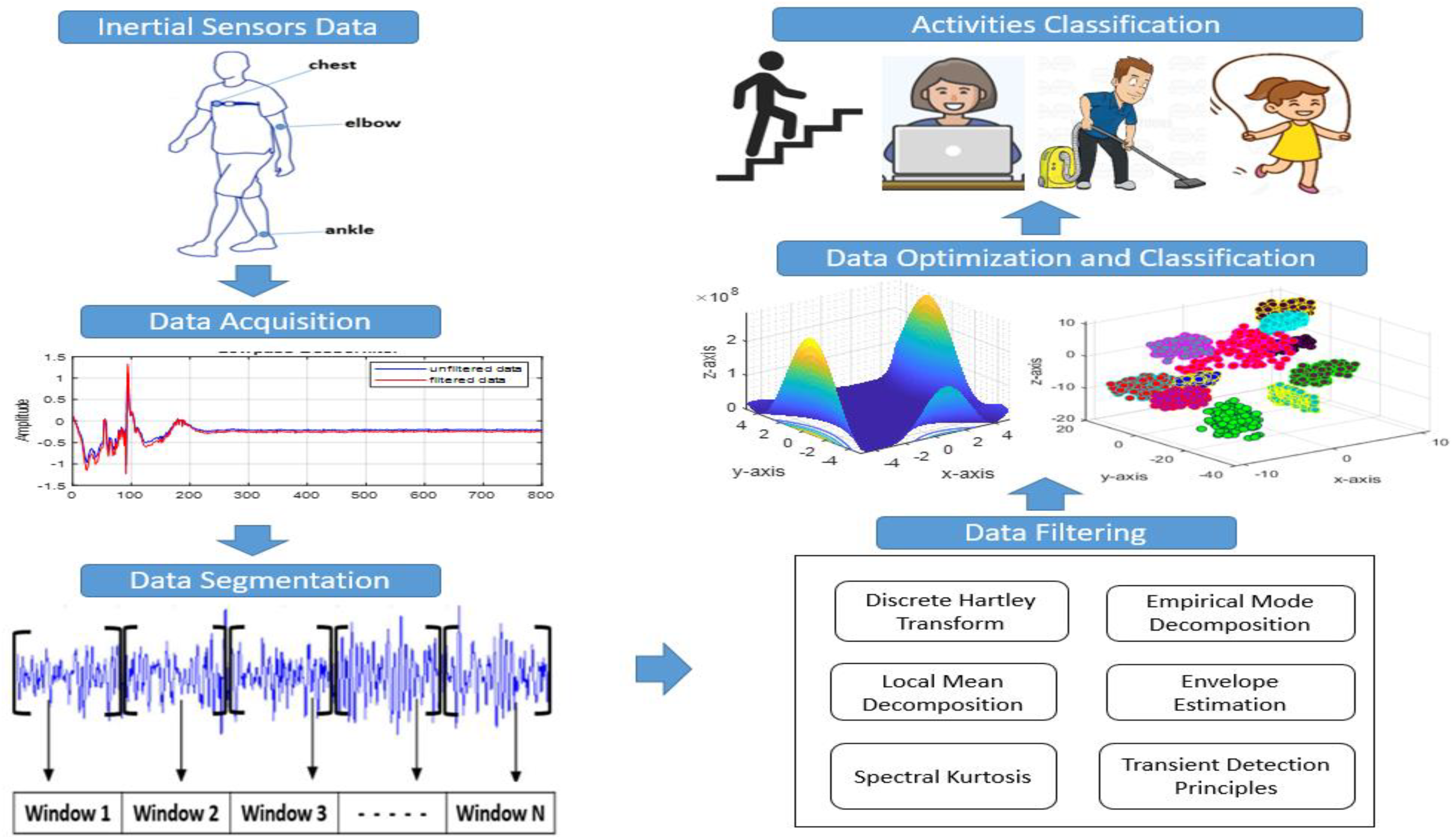
The proposed model has been integrated by passing the signal through a standardized model to achieve enhanced classification. The block diagram of the proposed HBM is shown in Figure 1. It includes five main steps, namely data acquisition, data segmentation and denoising, feature extraction, data optimization, and classification. The data of the signal is first segmented with a fixed window frame. The signal is refined using Chebyshev, Elliptic, and Bessel filters. Then, the filtered and denoised signals are used for the extraction of features. The extracted features include both frequency and time-domain features. Next, extracted features are optimized using a Probability Based Incremental Learning (PBIL) optimizer. Finally, the optimized data is classified using a K-Ary Tree Hashing (KATH) classifier.
3.1. Preprocessing Stage
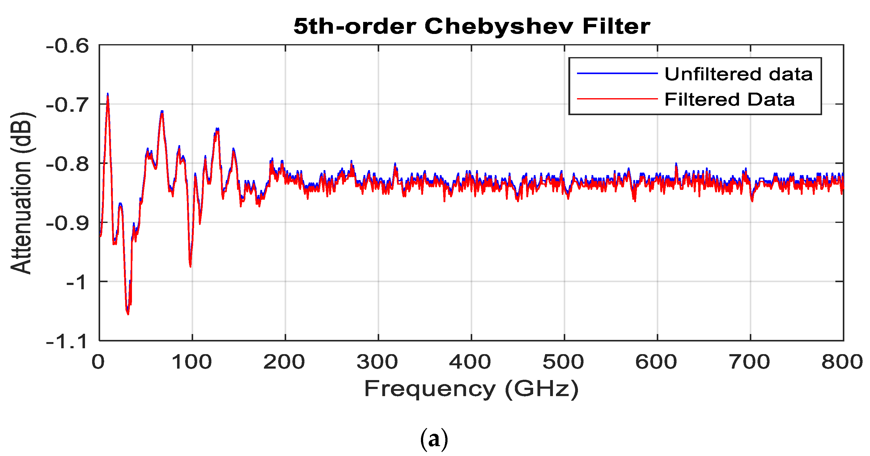
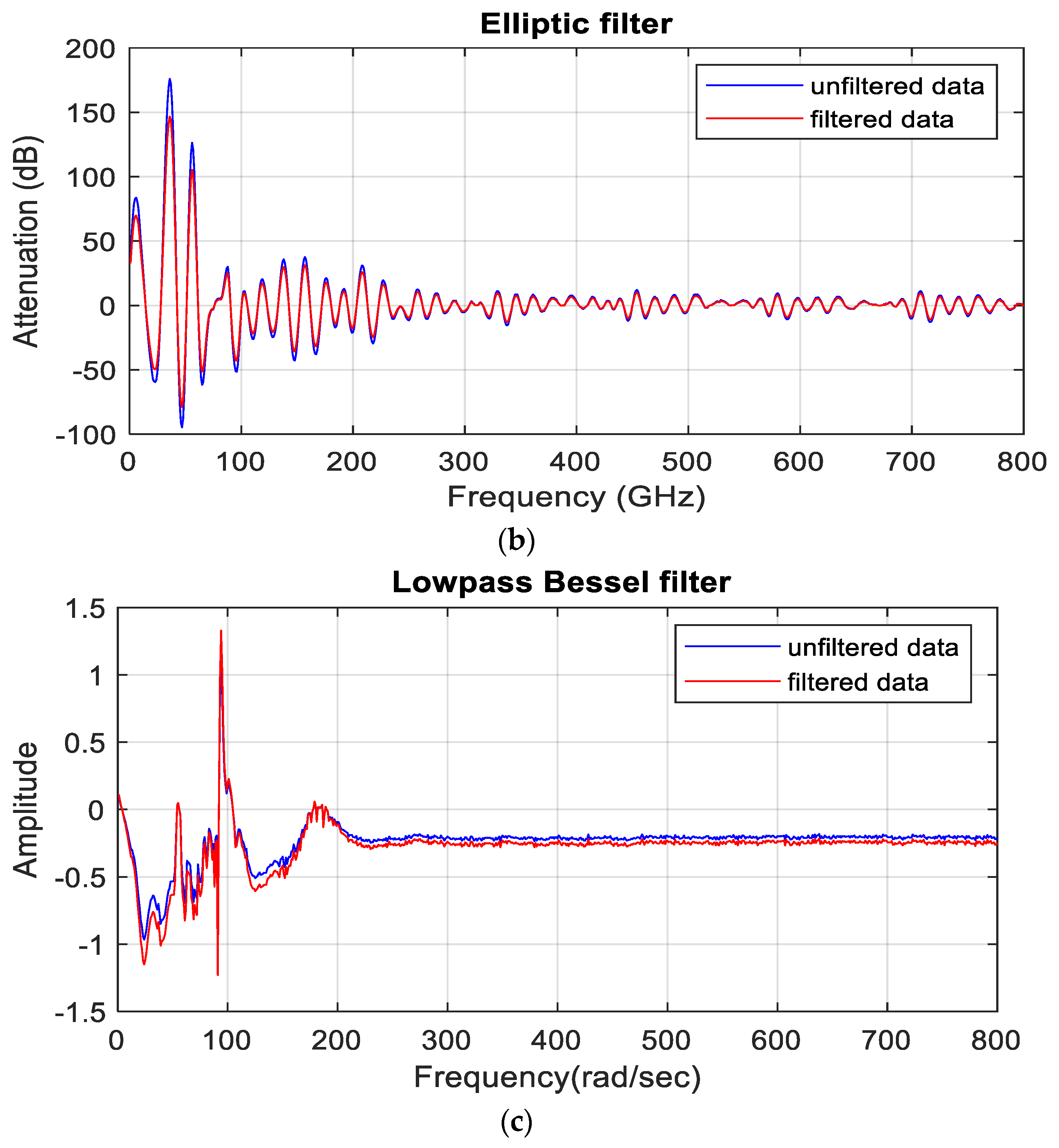
An inertial sensor, like an IMU sensor, is highly prone to error, so any unintentional change can alter the signal shape and complicate feature extraction. Therefore, signal data is first preprocessed using multiple filters such as Chebyshev, Elliptic, and Bessel filter. The Chebyshev filter removes power line interference, smooths the raw data, and increases the accuracy of the data (See Figure 2a). The Elliptic filter removes the random oddities in raw signals as shown in See Figure 2b. The Bessel filter preserves the shape of the filtered signals in the passband and eliminates the impulsive type of noise. The Bessel filter provides a better response than Chebyshev and Elliptic filter as illustrated in Figure 2. Meanwhile, the Bessel filter denoises the signal in the proposed model.
3.2. Windows Selection
A signal cannot be processed in a non-stationary form. Therefore, framing or windowing is needed to divide the signal into short stationary segments. In this way, each behavior can be accommodated to recognize different signal patterns. The three datasets used in this paper reflect different behavioral patterns. Human motion patterns such as ascending stairs, treadmill running, bicycling, and rope jumping in the DALIAC dataset required a short time duration frame to accurately analyze and predict the subject’s behavior.
Inertial signals are taken as a stream and subjected to feature extraction for the sensor data stream. Initially, the definitive parameters are considered, namely window selection into a fixed size for better recognition of signal patterns. Conventionally, a 4–5 s window has been utilized because the same pattern of the activity is followed in most of the databases [38,39,40]. In our case, due to the proposition to use a physical activities dataset that reveals more dynamicity in the data, the selection of the traditional approach was considered less effective and needs further analysis. While considering our data, different window sizes from 4 s to 9 s were chosen to quantify the effect of the varying window length on DALIAC, PAMPA2, and IM-LifeLog datasets, as shown in the Table 1. In the proposed model a 9 s window was used to obtain accurate results.
3.3. Features Extraction
In the features extraction methodology, we proposed a novel combination of features that included Discrete Hartley Transform, Local Mean Decomposition, Spectral Kurtosis, Transient Detection Principles, Envelope Estimation, and Empirical Mode Decomposition. Algorithm 1 defines the novel set of features as;
| Algorithm 1. Human Locomotion Feature Extraction. |
| Input: Inertial sensors data Accelerometer (x, y, z), Gyroscope (x, y, z), Magnetometer (x, y, z); Output: FeatureMatrix (vm1, vm2, vm3, ……………., vmN) FeatureMatrix ← [] WindowSize ← GetWindowSize () While signal data in (acc, gyro, mag) do FramedSignal ← WindowSignal (signal data, WindowSize) DHT ← Extract_DiscreteHartleyTransform (FramedSignal) LMD ← Extract_LocalMeanDecomposition (FramedSignal) SKT ← Extract_SpectralKurtosis (FramedSignal) TDP ← Extract_TransientDetectionPrinciples (FramedSignal) EET ← Extract_EnvelopeEstimation (FramedSignal) EMD ← Extract_EmpiricalDiscreteHartleyTransform (FramedSignal) FeatureMatrix.append (DHT, LMD, SKT, TDP, EET, EMD) return FeatureMatrix |
3.3.1. Discrete Hartley Transform Feature
The Discrete Hartley Transform (DHT) feature is an orthogonal transform that computes complex numbers Xn to accurately capture the behavior of the signal as a function of time. The real Xn_real and imaginary Xn_img part of the complex number represent the cosine and sine components in real numbers with embedded magnitude and phase information. The standard DHT is defined as;
where,
where N represents the total number of Discrete Hartley Transform of a sequence x(n), for 0 to N − 1. Figure 3 represents Discrete Hartley Transform of signal components.
3.3.2. Local Mean Decomposition Feature
Local Mean Decomposition (LMD) gradually and smoothly decomposes the complicated signal into many single components known as product functions (PFs). The PFs give the information of two important attributes: frequency and envelope of the signal from which a time-varying instantaneous frequency can be derived. The LMD process will continue until all the PFs components are formed, as shown in Figure 4. The following are the steps of the LMD method:
- Calculate the Local Mean Decomposition of the adjacent samples, i.e., ni and ni+1 of the signal as;
- Then, calculate the envelope estimation of the signal of the frame of the signal, i.e., ai
- Next, the calculated mean value m(t) is separated from the current sample x(t). Then, the frequency modulation signal s(t) is achieved by dividing the separated function g(t) from the envelope function a(t) as;
- Later on, all estimated envelops are multiplied to attain an envelope signal a(t).
- Next, the PFs components are obtained by multiplying the frequency modulated signal, i.e., s(t) and the envelope signal a(t) together.
- Finally, calculated PFs components are then subtracted from the original current sample to determine whether uk(t) is a monotonic function or not. If the result is not monotonic then all the above processes are repeated from the first step.
3.3.3. Spectral Kurtosis Feature
The Spectral Kurtosis (SKT) is the time-frequency domain method. It calculates the nearness arrangement of transients in the frequency domain by taking a proportion of peakedness and signal impulsiveness. Hence, it is a useful tool for characterizing non-stationary or non-Gaussian behavior in the frequency domain. The SKT is depicted as;
where fk is the frequency in Hertz, sk is the spectral value, µ1 and µ2 are the spectral centroid and spectral spread, respectively. The b1 and b2 are the band edges that calculate Spectral Kurtosis.
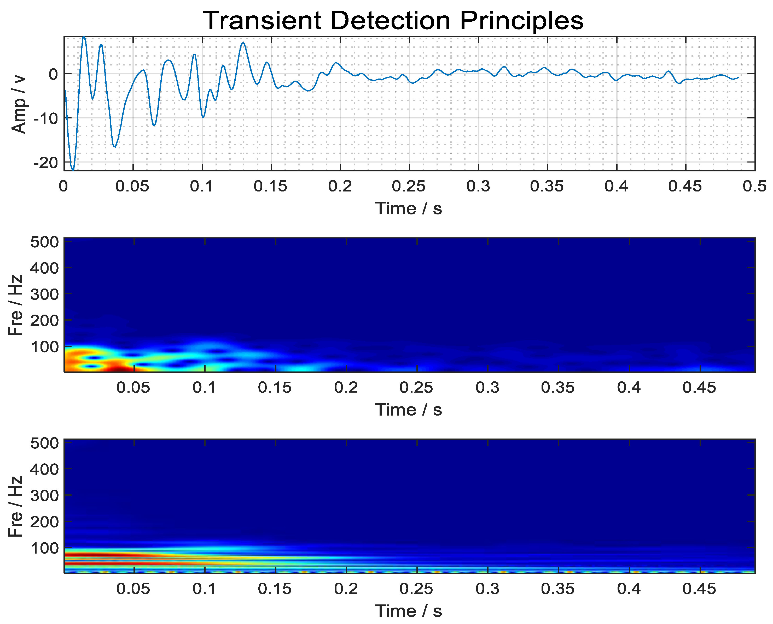
3.3.4. The Transient Detection Principles Feature
The Transient Detection Principles (TDP) eliminate the area of low background activity and detect transient events in the signal data. It detects the non-harmonic phase of a signal within short frames of the signal, as shown in Figure 3. The mean absolute value of the signal is selected as threshold value t, to eliminate the area of low background activity. The threshold t is calculated as;
where xi represents the samples of the signal and N is the total number of samples within a given frame.
3.3.5. Envelope Estimation Feature
The Hilbert transform envelope detector is used to detect the envelope of the amplitude of the signal. The envelope is calculated by first taking the square root of the differentiator f′(t). The resultant f′(t)2 is then summed up with the product of f(t) and f″(t). The square root is then fed with gain. Envelope estimation is shown in Figure 4. The final equation is defined as;
3.3.6. Empirical Mode Decomposition Feature
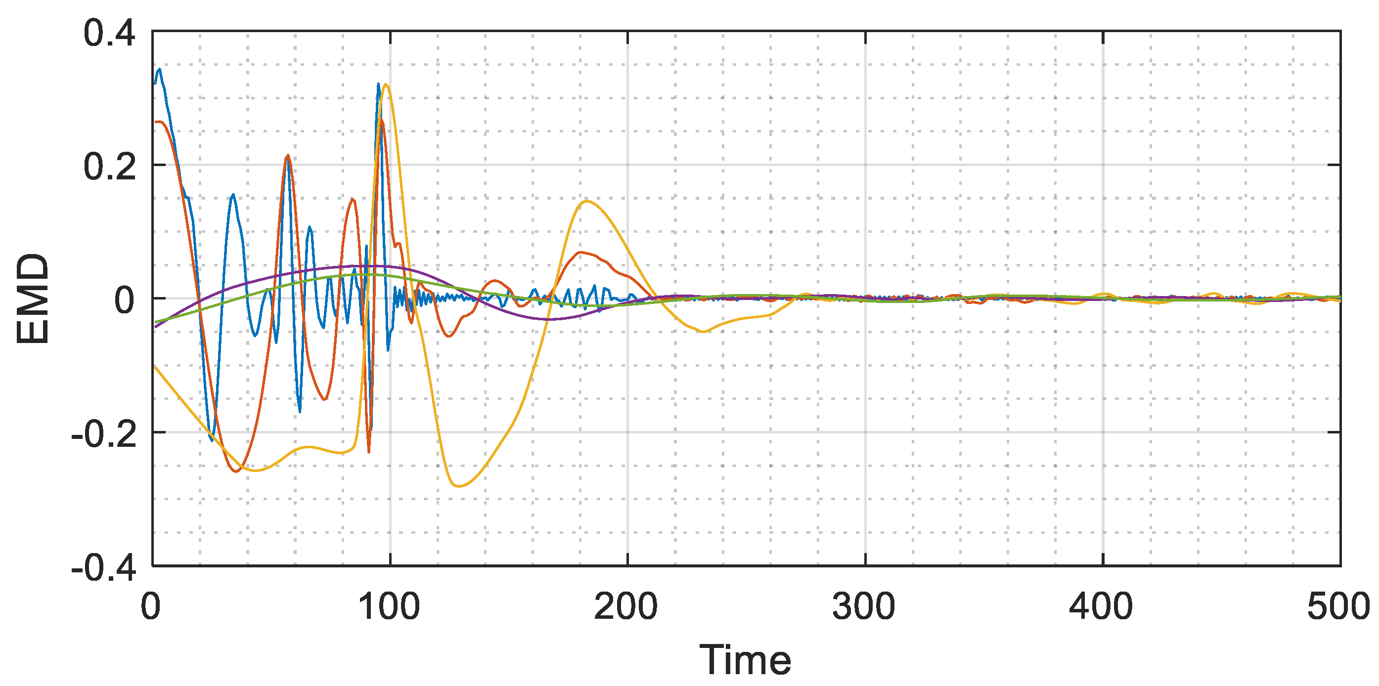
The Empirical Mode Decomposition (EMD) is an adaptive analysis method. It is a data-driven method that uses the characteristics of the signal to decompose its values. Moreover, it automatically and efficiently adjusts the scale of the signal. The decomposition process starts by first finding local maxima and minima values. Moreover, two important conditions are checked: Firstly, zero crossing of the signal should not exceed the value of one and, secondly, the local mean of the envelope of the signal should be close to zero. If both conditions are satisfied, we proceed further and extract the intrinsic mode function (IMF). The envelope of the signal is taken, and we extract the intrinsic mode function (IMF) from the signal, but only if zero-crossing does not exceed one and the local mean of envelope of the signal is close to zero, as shown in Figure 5. If it does not meet these two conditions, then the whole process is repeated until it satisfies the above-mentioned conditions. It is represented as;
where Emean is the mean of the upper envelope of the signal Eup, and the lower envelope of the signal Edown. The mean of the envelope Emean is subtracted from the original signal x(t) to get a decomposition of the signal d(t).
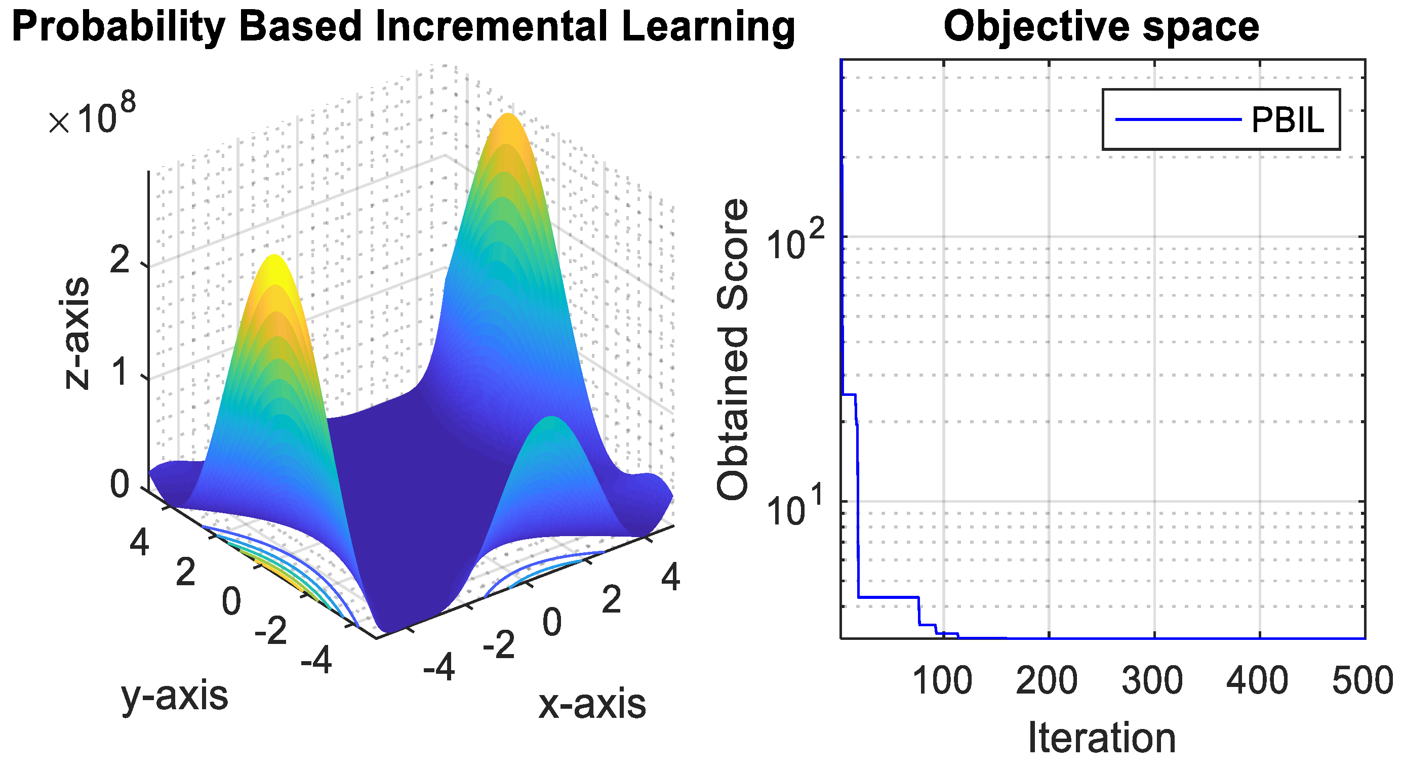
3.4. Optimization Algorithm: Probability Based Incremental Learning
Probability Based Incremental Learning (PBIL) is a combination of a genetic algorithm (GA) and competitive learning. GA is mostly known as a function optimizer that works on three complex operations, i.e., selection, crossover, and mutation [38]. These GA operations are theoretical and numerically complex. To overcome the disadvantage of GA, a PBIL algorithm is designed that works like a GA on a binary encoded representation of an optimal problem. The PBIL algorithm works on a real valued probability vector from which potential solutions are generated. The population of an individual is represented by a probability vector. It is defined as;
where, p1(xi) represents the probability of ith gene position that has obtained the value of 1. The PBIL vectors are initialized to 0.5 which produces uniform distribution with an equal probability of 1 and 0 for each bit of chromosomes. Thus, the chromosomes gradually shift toward the solution with highest fitness value [39].
The evolution process in PBIL works by generating M number of solutions on the basis of current probability vector p1(x). The results are then evaluated and N best solutions (N ≤ M) are selected to update the probability vector by using a Hebbian inspired rule. It is depicted as;
where a is the learning rate and it is represented as a ϵ (0,1]. After the probability vector is updated, a new set of solutions is generated by sampling from the new probability vector. The process is repeated until the probability vector for each bit position is either converged to 0.0 or 1.0.
The PBIL algorithm efficiently works on the data. Still, a major drawback of PBIL is that it often gets trapped in a local optimum as a single probability vector which is used to generate the complete population. To overcome this issue, the updated PBILs proposed in [41] are used in this paper. In the updated PBIL, each individual vector uses different probability vectors to generate its own children. Moreover, to further speed up the convergence, the neighborhood updates its probability vectors on a random basis, as shown in Figure 6. It is depicted as;
where LR is the learning rate, best(i) and neigbest(i) are the best solution of ith string. While, r is the random parameter selected from the interval of [0, 1].
3.5. K-Ary Tree Hashing Classifier
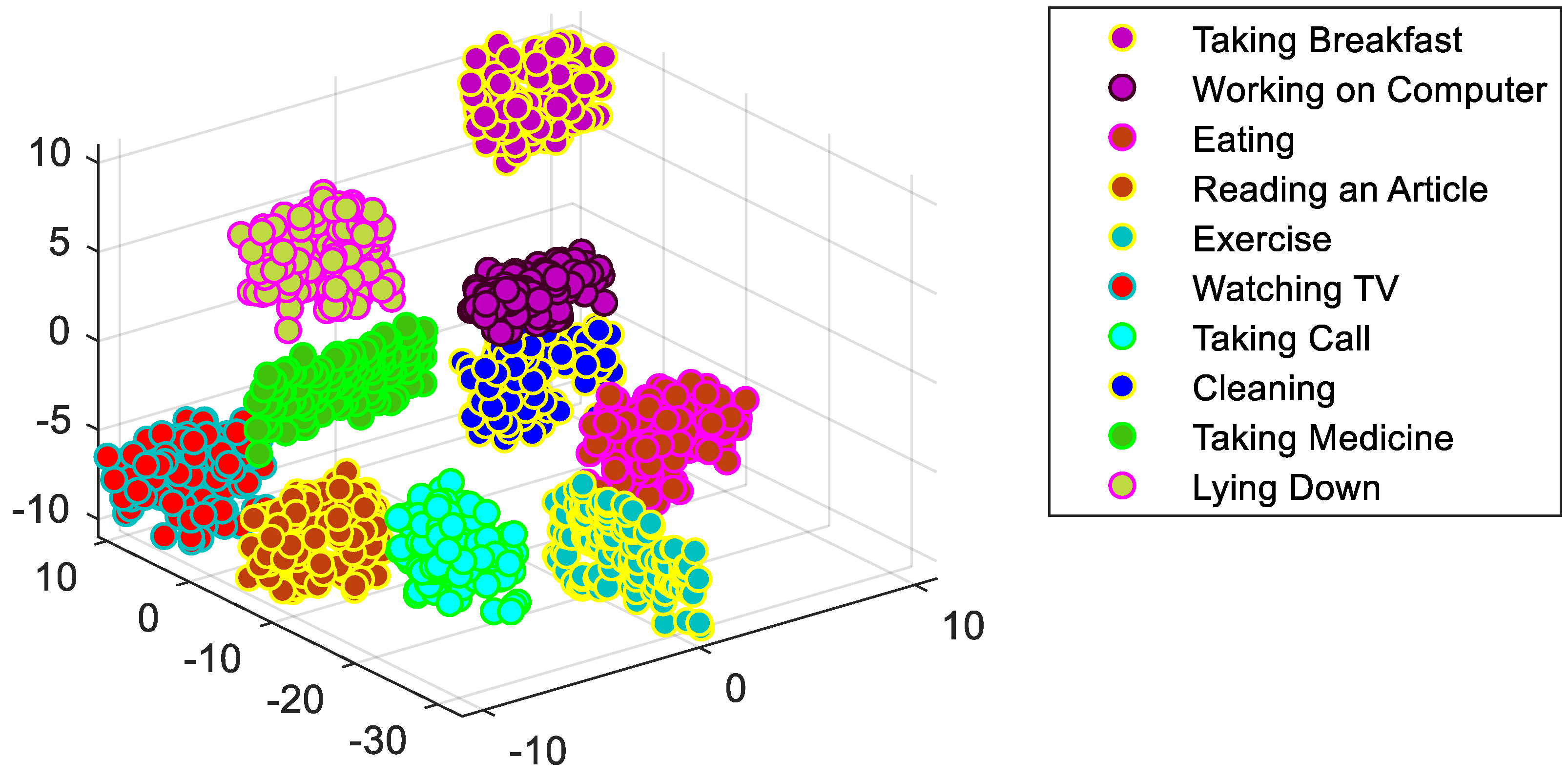
The K-Ary Tree Hashing (KATH) classifier is a graph classification algorithm that obtains competitive accuracy with a fast run time, especially for large scale graphs. The main idea of KATH is that the whole graph is projected on a set of optimized features in a common feature space without having any prior knowledge of subtree patterns. Later, a traversal table is constructed that keeps track of similar patterns within the optimized data. It performs recursive indexing for a N number of optimized data to generate (n − 1) depth optimized data to uniquely specify the patterns. Finally, MinHash is applied to classify the sub-patterns to discriminate against different human activities [42]. After analyzing the KATH algorithm, two favorable properties of KATH are obtained: Firstly, the bound of convergence rate tends to become tighter as the KATH algorithm steps into higher resolution. Secondly, the KATH kernel is robust in that it tolerates drift between graph chunks over a stream [43,44]. The experimental results show that KATH can classify data from significantly different activities other than the generic framework, e.g., SVM and logistic regression, as shown in Figure 7. Algorithm 1 depicts the pseudocode of the KATH algorithm. The input includes a graph represented by g = (ν, Ɛ,ℓ), the number of iterations is represented by R while M represents the feature space. The nodes ν are relabeled and only consider their neighboring nodes Nv to assign a new label ℓ(r). The traversal table is generated and stored in T. The algorithm works in three steps, as shown in Algorithm 2. The First Traversal Table is constructed (Lines 1–7), where each leaf is extended to new leaves (Lines 8–13) based on the indexing of optimized data. Finally, a MinHash scheme is applied (Lines 15–16) to classify the data into different human activities. The results of DALIAC, PAMAP2, and IM-LifeLog datasets at k iterations are depicted in Table 2. PCA (Principle Component Analysis) is used as a dimensional reduction algorithm to plot the clustering results in a 3D feature space. We construct a dxk dimensional transformation matrix W that allows us to map a sample vector x onto a new k-dimensional feature subspace that has fewer dimensions than the original d-dimensional feature space as shown in the below equation.
where x is the array of sample vectors from x1 to xd, and z is the array of sample vectors from z1 to zk in Rd and Rk dimensional space respectively.
| Algorithm 2. KATH Classifier. |
| Input: Output: 1: 2: 3: 4: fordo 5: 6: 7: end for 8: 9: 10: fordo 11: ifthen 12: 13: 14: end if 15: 16: |
4. Experimental Results and Analysis
4.1. Experimental Testing and Datasets Descriptions
A platform is established to evaluate the performance of the proposed methodology using inertial sensors to attain data on human daily life activities. All datasets are applied in real-time situations, especially in health care assessments of physical exercises and daily life-log routines. All datasets are evaluated using a Leave One Subject Out (LOSO) cross-validation method over training and testing data.
Three datasets are used for experimental evaluations. The DALIAC dataset [45] is taken from four sensors placed on the right hip, chest, right wrist, and left ankle of thirteen healthy subjects. The age of the subjects ranged between 8 to 26 years, and their weight ranged between 14 kg to 75 kg. Thirteen activities were performed by the participants: sitting, lying, standing, washing dishes, vacuuming, sweeping, walking, ascending stairs, descending stairs, treadmill running, bicycling on ergometer (50 W), bicycling on ergometer (100 W) and rope jumping.
The PAMAP2 dataset [46] was performed on IMUs inertial sensors that consist of accelerometer, gyroscope, and magnetometer signal values. Three IMU sensors are placed on the subject’s wrist, chest, and ankle. We performed experiments over thirteen activities: lying, sitting, standing, walking, running, cycling, nordic walking, watching TV, computer work, car driving, ascending stairs, descending stairs, and vacuum cleaning.
The IM-LifeLog dataset [47] is our self-annotated human life-logging dataset. Three IMU sensors were placed on the subject’s body at the ankle, elbow, and chest. A total of nine subjects performed ten activities: taking breakfast, working on computer, eating, reading an article, exercise, watching tv, taking call, cleaning, taking medicine, and lying down. Each activity was performed for one minute duration. The age of the participants ranged from 10 to 45 years and the weight range was 15 to 80 kg.
4.2. Hardware Platform
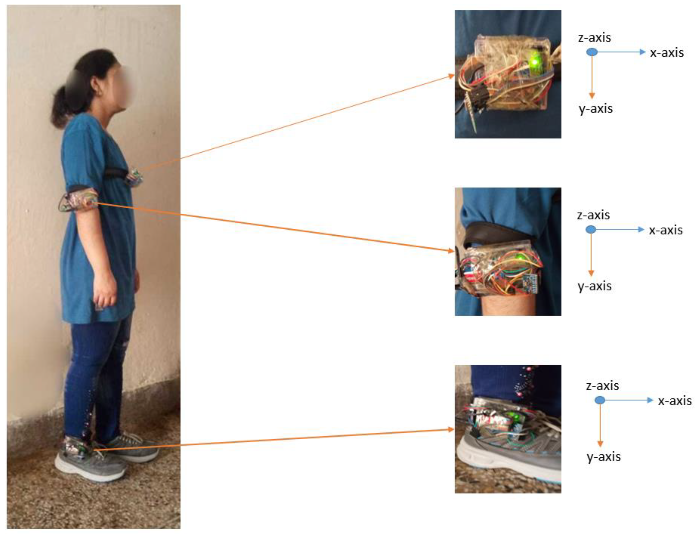
Three IMU sensors and an NRFL01 module were interfaced with Arduino UNO; these are known as the sender modules. The three sender modules were mounted on the participant’s ankle, elbow, and chest, as shown in Figure 8. The fourth setup is comprised of only the NRFL01 interfaced with an Arduino UNO, which is known as the receiver module. All three sender modules were mounted on the human body in order to send the IMU sensor data to the fourth module, the receiver modules. Arduino software (IDE) was used to develop the software for the complete setup. The fourth module, the receiver, was interfaced with a Visual studio 2015 application for simulation in the real-time environment. The IMU sensors consisted of a 3-axis accelerometer, a 3-axis gyroscope, and a 3-axis magnetometer in a small package. The main limitation in this setup was the 9-volt battery, which could only operate for up to two days. This limitation can be overcome by recharging or replacing the battery at appropriate times.
The accuracy of individual sensor groups with their location is investigated by placing the sensors at seven different locations, specifically, upper arm, elbow, wrist, chest, hip, thigh, and ankle. These configurations create 12 different combinations that are investigated using the proposed methodology. The sensors mounted at joint locations, wrist, ankle, and elbow, provide the information of 3D motion capture data regarding human body movement. The sensor mounted at the wrist captures the 3D rotation of hand movement. Similarly, by placing the sensor at the ankle position, four ankle movements can be monitored: plantar flexion (PF), dorsiflexion (DF), inversion (INV), and eversion (EVR) which are further used to capture the accurate leg movement. The results regarding the position of the sensors are evaluated and the best accuracy on our model is achieved by placing the sensors at the chest, elbow, and ankle as shown in Table 3. Hence, the elbow, ankle, and chest position are recommended for recognizing human activity classification.
4.3. Experimental Results and Evaluation
Experiments are conducted on three benchmark datasets to evaluate the performance of the proposed HBM model. Table 4 presents the confusion matrix of 13 activities in the DALIAC dataset, where accuracy of 94.23% was obtained. On the other hand, Table 5 depicts the mean accuracy of 94.07% over 13 different activities in the PAMAP2 dataset. Table 6 shows the confusion matrix of the IM-LifeLog dataset over 10 activities, where accuracy of 96.40% over the KATH classifier was achieved. Finally, Table 7 presents the comparison results of the proposed approach over DALIAC, PAMAP2, and IM-LifeLog datasets, respectively.
5. Conclusions and Future Works
In this paper, we proposed novel frequency and time domain features for an HBM system that recognizes life-logging activities transmitted from inertial IMU sensors. These features examined the Discrete Hartley Transform, Local Mean Decomposition, Spectral Kurtosis, Transient Detection Principles, Envelope Estimation, and Empirical Mode Decomposition features. Such features are optimized using Probability Based Incremental Learning (PBIL) and are then classified using a K-Ary based Tree Hashing classifier (KATH). The proposed model is evaluated on three benchmark datasets that give an accuracy of 94.23%, 94.07%, 96.40% over DALIAC, PAMAP2, and self-annotated IM-LifeLog datasets, respectively. Our proposed methodology achieved remarkable accuracy rates over current state-of-the-art methods.
As future work, the proposed method will be further improved by adding features from different domains. Additionally, we are planning to develop datasets for elderly healthcare using inertial and optical sensors.
Author Contributions
Conceptualization, M.B.; methodology, M.B. and A.J.; software, M.B.; validation, A.J.; formal analysis, K.K.; resources, A.J. and K.K.; writing—review and editing, A.J. and K.K.; funding acquisition, A.J. and K.K. All authors have read and agreed to the published version of the manuscript.
Funding
This research was supported by Basic Science Research Program through the National Research Foundation of Korea (NRF) funded by the Ministry of Education (no. 2018R1D1A1A02085645).
Conflicts of Interest
The authors declare no conflict of interest.
References
- Ranasinghe, S.; Machot, F.A.; Mayr, H.C. A review on applications of activity recognition systems with regard to performance and evaluation. Int. J. Distrib. Sens. Netw. 2016, 12, 1–22. [Google Scholar] [CrossRef] [Green Version]
- Susan, S.; Agrawal, P.; Mittal, M.; Bansal, S. New shape descriptor in the context of edge continuity. Caai Trans. Intell. Technol. 2019, 4, 101–109. [Google Scholar] [CrossRef]
- Shokri, M.; Tavakoli, K. A review on the artificial neural network approach to analysis and prediction of seismic damage in infrastructure. Int. J. Hydromechatronics 2019, 4, 178–196. [Google Scholar] [CrossRef]
- Priya, L.G.G.; Domnic, S. Walsh–Hadamard Transform Kernel-Based Feature Vector for Shot Boundary Detection. IEEE Trans. Image Process. 2014, 23, 5187–5197. [Google Scholar]
- Tingting, Y.; Junqian, W.; Lintai, W.; Yong, X. Three-stage network for age estimation. Caai Trans. Intell. Technol. 2019, 4, 122–126. [Google Scholar] [CrossRef]
- Wiens, T. Engine speed reduction for hydraulic machinery using predictive algorithms. Int. J. Hydromechatronics 2019, 2, 16–31. [Google Scholar] [CrossRef]
- Ichikawa, F.; Chipchase, J.; Grignani, R. Where’s the phone? A study of mobile phone location in public spaces. In Proceedings of the 2005 IEE International Conference on Mobile Technology, Guangzhou, China, 15–17 November 2005; pp. 142–148. [Google Scholar]
- Zhu, C.; Miao, D. Influence of kernel clustering on an RBFN. Caai Trans. Intell. Technol. 2019, 4, 255–260. [Google Scholar] [CrossRef]
- Osterland, S.; Weber, J. Analytical analysis of single-stage pressure relief valves. Int. J. Hydromechatronics 2019, 2, 32–53. [Google Scholar] [CrossRef]
- Zhang, M.; Sawchuk, A.A. A feature selection-based framework for human activity recognition usingwearable multimodal sensors. In Proceedings of the 6th International Conference on Body Area Networks, Beijing, China, 7–8 November 2011; pp. 92–98. [Google Scholar]
- Hu, T.; Zhu, X.; Wang, S.; Duan, L. Human interaction recognition using spatial-temporal salient feature. Multimed Tools Appl. 2018, 78, 1–21. [Google Scholar] [CrossRef]
- Anithaa, U.; Narmadhab, R.; Sumanthc, R.D.; Kumarc, D.N. Robust Human Action Recognition System via Image Processing. Procedia Comput. Sci. 2020, 167, 870–877. [Google Scholar]
- Mahmood, M.; Jalal, A.; Kim, K. WHITE STAG model: Wise human interaction tracking and estimation (WHITE) using spatio-temporal and angular-geometric (STAG) descriptors. Multimed. Tools Appl. 2019, 79, 6919–6950. [Google Scholar] [CrossRef]
- Sreela, S.R.; Idicula, S.M. Action Recognition in Still Images using Residual Neural Network Features. Proc. Comput. Sci. 2018, 143, 563–569. [Google Scholar] [CrossRef]
- Jalal, A.; Uddin, M.Z.; Kim, T.-S. Depth Video-based Human Activity Recognition System Using Translation and Scaling Invariant Features for Life Logging at Smart Home. IEEE Trans. Consum. Electr. 2018, 58, 863–871. [Google Scholar] [CrossRef]
- Weng, E.J.; Fu, L.C. On-Line Human Action Recognition by Combining Joint Tracking and Key Pose Recognition. In Proceedings of the IEEE/RSJ International Conference on Intelligent Robots and Systems, Vilamoura, Portugal, 7–12 October 2012. [Google Scholar]
- Jalal, A.; Quaid, M.A.K.; Hasan, A.S. Wearable Sensor-Based Human Behavior Understanding and Recognition in Daily Life for Smart Environments. In Proceedings of the International Conference on Frontiers of Information Technology (FIT), Islamabad, Pakistan, 17–19 December 2018. [Google Scholar]
- Tahir, S.B.; Jalal, A.; Batool, M. Wearable Sensors for Activity Analysis using SMO-based Random Forest over Smart home and Sports Datasets. In Proceedings of the 3rd International Conference on Advancements, Lahore, Pakistan, 17–19 February 2020. [Google Scholar]
- Batool, M.; Jalal, A.; Kim, K. Sensors Technologies for Human Activity Analysis Based on SVM Optimized by PSO Algorithm. In Proceedings of the IEEE conference on International Conference on Applied and Engineering Mathematics, Taxila, Pakistan, 27–29 August 2019. [Google Scholar]
- Shahar, N.; Ghazali, N.F.; Asari, M.A.; Swee, T.T. Wearable Inertial Sensor for Human Activity Recognition in Field Hockey: Influence of Sensor Combination and Sensor Location. In Proceedings of the 2nd Joint International Conference on emerging computing technology and sports (JICETS), Bandung, Indonesia, 25–27 November 2019. [Google Scholar]
- Uddin, M.T.; Uddin, M.A. A Guided Random Forest based Feature Selection Approach for Activity Recognition. In Proceedings of the 2nd Int’l Conf. on Electrical Engineering and Infonnation & Communication Technology (ICEEICT), Dhaka, Bangladesh, 21–23 May 2015. [Google Scholar]
- Iqbal, A.; Ullah, F.; Anwar, H.; Kiran, S. Wearable Internet-of-Things platform for human activity recognition and health care. Int. J. Distrib. Sens. Netw. 2020, 16. [Google Scholar] [CrossRef]
- Adama, D.A.; Lotfi, A.; Langensiepen, C.; Lee, K.; Trindade, P. Human activity learning for assistive robotics using a classifier ensemble. Soft Comput. 2018, 22, 7027–7039. [Google Scholar] [CrossRef] [Green Version]
- Ijjina, E.P.; Mohan, K. Human action recognition in RGB-D videos using motion sequence information and deep learning. Pattern Recognit. 2017. [Google Scholar] [CrossRef]
- Cippitelli, E.; Gasparrini, S.; Gambi, E.; Spinsante, S. A Human Activity Recognition System Using Skeleton Data from RGBD Sensors. Comput. Intell. Neurosci. 2016. [Google Scholar] [CrossRef] [Green Version]
- Koppula, H.S.; Gupta, R.; Saxena, A. Learning Human Activities and Object Affordances from RGB-D Videos. arXiv 2013, arXiv:1210.1207. [Google Scholar] [CrossRef] [Green Version]
- Jalal, A.; Kim, Y.H.; Kim, Y.J.; Kamal, S.; Kim, D. Robust human activity recognition from depth video using spatiotemporal multi-fused features. Pattern Recognit. 2017, 295–308. [Google Scholar] [CrossRef]
- Zanfir, M.; Leordeanu, M.; Sminchisescu, C. The moving pose: An efficient 3d kinematics descriptor for low-latency action recognition and detection. In Proceedings of the IEEE International Conference on Computer Vision, Sydney, Australia, 1–8 December 2013; pp. 2752–2759. [Google Scholar]
- Mannini, A.; Rosenberger, M.; Haskell, W.L.; Sabatini, A.M.; Intille, S.S. Activity recognition in youth using single accelerometer placed at wrist or ankle. Med. Sci. Sports Exercise. 2017, 49. [Google Scholar] [CrossRef] [Green Version]
- Akram, B.; Pomplun, M.; Tran, D.A. A Study on Human Activity Recognition Using Accelerometer Data from Smartphones; Elsevier Procedia Computer Science: Amsterdam, The Netherlands, 2014; Volume 34. [Google Scholar]
- Tahir, S.B.; Jalal, A.; Kim, K. Wearable Inertial Sensors for Daily Activity Analysis Based on Adam Optimization and the Maximum Entropy Markov Model. Entropy 2020, 22, 579. [Google Scholar] [CrossRef]
- Cao, L.; Wang, Y.; Zhang, B.; Jin, Q.; Vasilakos, A.V. GCHAR: An efficient Group-based Context—Aware human activity recognition on smartphone. J. Parallel Distrib. Comput. 2018, 118, 67–80. [Google Scholar] [CrossRef]
- Golestani, N.; Moghaddam, M. Human activity recognition using magnetic induction-based motion signals and deep recurrent neural networks. Nat. Commun. 2020, 11, 1–11. [Google Scholar] [CrossRef] [PubMed]
- Zebin, T.; Scully, P.J.; Ozanyan, K.B. Human activity recognition with inertial sensors using a deep learning approach. In Proceedings of the IEEE Sensors, Orlando, FL, USA, 30 October–3 November 2016. [Google Scholar]
- Murahari, V.S.; Plotz, T. On attention models for human activity recognition. In Proceedings of the 2018 ACM International Symposium on Wearable Computers, Singapore, 8–12 October 2018; pp. 100–103. [Google Scholar]
- Xi, R.; Li, M.; Hou, M.; Fu, M.; Qu, H.; Liu, D. Deep dilation on multimodality time series for human activity recognition. IEEE Access. 2018, 6, 53381–53396. [Google Scholar] [CrossRef]
- Hammerla, Y.; Halloran, S.; Ploetz, T. Deep convolutional and recurrent models for human activity recognition using wearables. arXiv 2016, arXiv:1604.08880. [Google Scholar]
- Kulkarni, R.G. Synthesis of a new signal processing window. Electr. Lett. 2019, 55, 1108–1110. [Google Scholar] [CrossRef]
- Bonomi, A.G.; Goris, A.H.C.; Yin, B.; Westerterp, K.R. Detection of type, duration, and intensity of physical activity using an accelerometer. Med. Sci. Sports Exerc. 2009, 41, 1770–1777. [Google Scholar] [CrossRef]
- Chifu, E.S.; Chifu, V.R.; Pop, C.B.; Vlad, A.; Salomie, I. Machine Learning Based Technique for Detecting Daily Routine and Deviations. In Proceedings of the 2018 IEEE 14th International Conference on Intelligent Computer Communication and Processing (ICCP), Cluj-Napoca, Romania, 6–8 September 2018; pp. 183–189. [Google Scholar] [CrossRef]
- Yang, S.Y.; Ho, S.L.; Ni, G.Z.; Machado, J.M.; Wong, K.F. A New Implementation of Population Based Incremental Learning Method for Optimization Studies in Electromagnetics. In Proceedings of the 12th Biennial IEEE Conference on Electromagnetic Field Computation, Miami, FL, USA, 30 April–3 May 2006; p. 163. [Google Scholar] [CrossRef]
- Quaid, M.; Jalal, A. Wearable Sensors based Human Behavioral Pattern Recognition using Statistical Features and Reweighted Genetic Algorithm. Multimed. Tools Appl. 2020, 79, 6061–6083. [Google Scholar] [CrossRef]
- Ahmed, N.; Rafiq, J.I.; Islam, M.R. Enhanced Human Activity Recognition Based on Smartphone Sensor Data Using Hybrid Feature Selection Model. Sensors 2020, 20, 317. [Google Scholar] [CrossRef] [Green Version]
- Shervashidze, N.; Schweitzer, P.; Leeuwen, E.J.V.; Mehlhorn, K.; Borgwardt, K.M. Weisfeiler-lehman graph kernels. J. Mach. Learn. Res. 2011, 12, 2539–2561. [Google Scholar]
- Vaquette, G.; Orcesi, A.; Lucat, L.; Achard, C. The Daily Home Life Activity Dataset. A High Semantic Activity Dataset for Online Recognition. In Proceedings of the 12th IEEE International Conference on Automatic Face & Gesture Recognition (FG 2017), Washington, DC, USA, 30 May–3 June 2017. [Google Scholar]
- Arif, M.; Kattan, A. Physical activities monitoring using wearable acceleration sensors attached to the body. PLoS ONE 2015, 10, e0130851. [Google Scholar] [CrossRef] [Green Version]
- Intelligent Media Center (IMC). Available online: http://portals.au.edu.pk/imc/Pages/Datasets.aspx (accessed on 19 September 2020).
- Zdravevski, E.; Lameski, P.; Trajkovik, V. Improving activity recognition accuracy in ambient-assisted living systems by automated feature engineering. IEEE Access. 2017, 5, 5262–5280. [Google Scholar] [CrossRef]
- Zaki, Z.; Muhammad, A.; Wakil, K.; Sher, F. Logistic regression based human activities recognition. J. Mech. Contin. Math. Sci. 2020. [Google Scholar] [CrossRef]
- Heroy, A.M.; Gill, Z.; Sprague, S.; Stroud, D.; Santerre, J. Stationary Exercise Classification using IMUs and Deep Learning. SMU Data Sci. Rev. 2020, 20, 1. [Google Scholar]
- Priyadharshini, J.M.H.; Kavitha, S.; Bharathi, B. Classification and analysis of human activities. In Proceedings of the International Conference on Communication and Signal Processing (ICCSP), Chennai, India, 6–8 April 2017; pp. 1207–1211. [Google Scholar] [CrossRef]
Figure 1.
Block diagram of the proposed model.

Figure 2.
Initial preprocessing. (a) 5th order Chebyshev filter, (b) Elliptic filter and (c) Low pass Bessel filter.
Figure 2.
Initial preprocessing. (a) 5th order Chebyshev filter, (b) Elliptic filter and (c) Low pass Bessel filter.


Figure 3.
Transient Detection Principles of signal data over the PAMPA2 dataset.

Figure 4.
Envelope estimation of signal data over the PAMPA2 dataset.

Figure 5.
Empirical mode decomposition of the signal data.

Figure 6.
Empirical mode decomposition of signal data.

Figure 7.
K-Ary Tree Hashing Classifier of optimized data over IM-LifeLog dataset.

Figure 8.
Wearable sensors mounted on the human body at the chest, elbow and ankle position in IM-LifeLog dataset.
Figure 8.
Wearable sensors mounted on the human body at the chest, elbow and ankle position in IM-LifeLog dataset.


Table 1.
Adaptive window size selection over DALIAC, PAMPA2, and IM-LifeLog datasets.
| Datasets | Four Second | Five Second | Six Second | Seven Second | Eight Second | Nine Second |
|---|---|---|---|---|---|---|
| DALIAC | 72.47% | 76.35% | 83.88% | 84.70% | 92.01% | 94.23% |
| PAMPA2 | 70.66% | 73.40% | 81.06% | 88.91% | 90.22% | 94.07% |
| IM-LifeLog | 74.54% | 72.87% | 86.55% | 82.35% | 94.12% | 96.40% |
Table 2.
K-Ary tree hashing implementation over DALIAC, PAMAP2 and IM-LifeLog datasets.
| Iterations | DALIAC | PAMAP2 | IM-LifeLog | |||
|---|---|---|---|---|---|---|
| Kth | Accuracy Rate | Loss Rate | Accuracy Rate | Loss Rate | Accuracy Rate | Loss Rate |
| 1 | 0.697 | 0.302 | 0.652 | 0.347 | 0.629 | 0.370 |
| 2 | 0.700 | 0.299 | 0.745 | 0.254 | 0.645 | 0.354 |
| 3 | 0.746 | 0.253 | 0.786 | 0.213 | 0.686 | 0.313 |
| 4 | 0.782 | 0.217 | 0.788 | 0.211 | 0.768 | 0.231 |
| 5 | 0.780 | 0.219 | 0.789 | 0.210 | 0.769 | 0.230 |
| 6 | 0.778 | 0.221 | 0.787 | 0.212 | 0.777 | 0.222 |
| 7 | 0.804 | 0.195 | 0.790 | 0.209 | 0.790 | 0.209 |
| 8 | 0.812 | 0.187 | 0.791 | 0.208 | 0.861 | 0.138 |
| 9 | 0.820 | 0.179 | 0.800 | 0.199 | 0.899 | 0.100 |
| 10 | 0.834 | 0.165 | 0.823 | 0.176 | 0.923 | 0.076 |
| 11 | 0.828 | 0.171 | 0.844 | 0.155 | 0.934 | 0.065 |
| 12 | 0.828 | 0.171 | 0.869 | 0.130 | 0.946 | 0.053 |
| 13 | 0.837 | 0.162 | 0.873 | 0.126 | 0.944 | 0.055 |
| 14 | 0.830 | 0.169 | 0.893 | 0.106 | 0.953 | 0.046 |
| 15 | 0.840 | 0.159 | 0.898 | 0.101 | 0.958 | 0.041 |
| 16 | 0.859 | 0.140 | 0.899 | 0.100 | 0.964 | 0.035 |
| 17 | 0.863 | 0.136 | 0.909 | 0.090 | 0.923 | 0.076 |
| 18 | 0.869 | 0.130 | 0.939 | 0.060 | 0.959 | 0.040 |
| 19 | 0.873 | 0.126 | 0.943 | 0.056 | 0.968 | 0.031 |
| 20 | 0.875 | 0.124 | 0.945 | 0.054 | 0.951 | 0.048 |
| 21 | 0.883 | 0.116 | 0.953 | 0.046 | 0.953 | 0.046 |
| 22 | 0.884 | 0.115 | 0.884 | 0.115 | 0.960 | 0.039 |
| 23 | 0.890 | 0.109 | 0.897 | 0.102 | 0.961 | 0.038 |
| 24 | 0.894 | 0.105 | 0.898 | 0.101 | 0.961 | 0.038 |
| 25 | 0.895 | 0.104 | 0.902 | 0.097 | 0.960 | 0.039 |
| 26 | 0.896 | 0.103 | 0.899 | 0.100 | 0.961 | 0.038 |
| 27 | 0.897 | 0.102 | 0.901 | 0.098 | 0.962 | 0.037 |
| 28 | 0.898 | 0.101 | 0.922 | 0.077 | 0.962 | 0.037 |
| 29 | 0.926 | 0.073 | 0.928 | 0.071 | 0.963 | 0.036 |
| 30 | 0.932 | 0.067 | 0.916 | 0.083 | 0.963 | 0.036 |
| 31 | 0.941 | 0.058 | 0.935 | 0.064 | 0.963 | 0.036 |
| 32 | 0.940 | 0.059 | 0.938 | 0.061 | 0.964 | 0.035 |
| 33 | 0.942 | 0.057 | 0.940 | 0.059 | 0.964 | 0.035 |
Table 3.
Sensors location at different body position.
| Sensors Location | DALIAC | PAMPA2 | IM-LifeLog |
|---|---|---|---|
| Wrist + Thigh + Hip | 72.47% | 76.35% | 83.88% |
| Wrist + Thigh + Chest | 90.66% | 93.40% | 91.06% |
| Wrist + Ankle + Hip | 88.61% | 89.08% | 84.34% |
| Wrist + Ankle + Chest | 79.09% | 88.17% | 79.42% |
| Upper Arm + Thigh + Hip | 74.54% | 92.87% | 76.55% |
| Upper Arm + Thigh + Chest | 89.25% | 73.36% | 89.59% |
| Upper Arm + Ankle + Hip | 74.69% | 79.50% | 86.69% |
| Upper Arm + Ankle + Chest | 91.85% | 89.32% | 88.58% |
| Elbow + Thigh + Hip | 88.04% | 91.02% | 87.40% |
| Elbow + Ankle + Hip | 76.03% | 84.09% | 93.97% |
| Elbow + Thigh + Chest | 90.79% | 78.61% | 82.42% |
| Elbow + Ankle + Chest | 94.23% | 94.07% | 96.40% |
Table 4.
Confusion matrix of human behavior modeling (HBM) accuracies over DALIAC dataset.
| Dynamic Activities | SI | LY | ST | WD | VC | SW | WK | AS | DS | TR | BF | BT | RJ |
|---|---|---|---|---|---|---|---|---|---|---|---|---|---|
| SI | 0.98 | 0 | 0.02 | 0 | 0 | 0 | 0 | 0 | 0 | 0 | 0 | 0 | 0 |
| LY | 0.02 | 0.96 | 0.01 | 0 | 0 | 0.01 | 0 | 0 | 0 | 0 | 0 | 0 | 0 |
| ST | 0.02 | 0.01 | 0.97 | 0 | 0 | 0 | 0 | 0 | 0 | 0 | 0 | 0 | 0 |
| WD | 0 | 0 | 0 | 0.93 | 0.03 | 0.01 | 0.01 | 0 | 0 | 0 | 0 | 0 | 0.02 |
| VC | 0 | 0 | 0 | 0.01 | 0.95 | 0.03 | 0.01 | 0 | 0 | 0 | 0 | 0 | 0 |
| SW | 0 | 0 | 0 | 0 | 0 | 0.98 | 0 | 0.01 | 0.01 | 0 | 0 | 0 | 0 |
| WK | 0 | 0 | 0 | 0 | 0.02 | 0 | 0.96 | 0.01 | 0.01 | 0 | 0 | 0 | 0 |
| AS | 0 | 0 | 0 | 0 | 0.04 | 0 | 0.01 | 0.91 | 0.03 | 0 | 0 | 0 | 0 |
| DS | 0 | 0 | 0 | 0 | 0.01 | 0 | 0 | 0.04 | 0.92 | 0 | 0 | 0.03 | 0 |
| TR | 0 | 0 | 0 | 0 | 0 | 0 | 0.01 | 0 | 0 | 0.94 | 0 | 0 | 0.05 |
| BF | 0 | 0 | 0 | 0 | 0 | 0.02 | 0 | 0.03 | 0 | 0 | 0.91 | 0.03 | 0 |
| BT | 0 | 0 | 0 | 0 | 0.01 | 0 | 0.03 | 0 | 0 | 0 | 0.06 | 0.90 | 0 |
| RJ | 0 | 0 | 0 | 0.01 | 0 | 0 | 0 | 0 | 0 | 0.05 | 0 | 0 | 0.94 |
| Mean Accuracy = 94.23% | |||||||||||||
SI = Sitting, LY = Lying, ST = Standing, WD = Washing dishes, VC = Vacuuming, SW = Sweeping, WK = Walking, AS = Ascending stairs, DS = Descending stairs, TR = Treadmill running, BF = Bicycling on ergometer (50 W), BT = Bicycling on ergometer (100 W), RJ = Rope Jumping.
Table 5.
Confusion matrix of HBM accuracies over PAMAP2 dataset.
| Dynamic Activities | LY | SI | ST | WK | RN | CY | NW | WT | CW | CD | AS | DS | VC |
|---|---|---|---|---|---|---|---|---|---|---|---|---|---|
| LY | 0.96 | 0.02 | 0.01 | 0 | 0 | 0 | 0 | 0.01 | 0 | 0 | 0 | 0 | 0 |
| SI | 0 | 0.98 | 0.02 | 0 | 0 | 0 | 0 | 0 | 0 | 0 | 0 | 0 | 0 |
| ST | 0.01 | 0.02 | 0.97 | 0 | 0 | 0 | 0 | 0 | 0 | 0 | 0 | 0 | 0 |
| WK | 0 | 0 | 0 | 0.94 | 0.03 | 0 | 0.02 | 0 | 0 | 0 | 0 | 0 | 0.01 |
| RN | 0 | 0 | 0 | 0.04 | 0.92 | 0 | 0.02 | 0 | 0 | 0 | 0.01 | 0.01 | 0 |
| CY | 0 | 0 | 0 | 0 | 0 | 0.95 | 0 | 0 | 0.02 | 0.02 | 0 | 0 | 0.01 |
| NW | 0 | 0 | 0 | 0.05 | 0 | 0 | 0.94 | 0 | 0 | 0 | 0 | 0 | 0.01 |
| WT | 0 | 0.01 | 0 | 0 | 0 | 0 | 0 | 0.96 | 0.02. | 0.01 | 0 | 0 | 0 |
| CW | 0 | 0 | 0 | 0 | 0 | 0.01 | 0 | 0.05 | 0.92 | 0.02 | 0 | 0 | 0 |
| CD | 0 | 0.02 | 0 | 0 | 0 | 0 | 0 | 0.02 | 0.03 | 0.93 | 0 | 0 | 0 |
| AS | 0 | 0 | 0 | 0 | 0.02 | 0 | 0.02 | 0 | 0 | 0 | 0.92 | 0.03 | 0.01 |
| DS | 0 | 0 | 0 | 0 | 0.03 | 0 | 0.04 | 0 | 0 | 0 | 0.06 | 0.87 | 0 |
| VC | 0 | 0 | 0 | 0 | 0 | 0 | 0.01 | 0 | 0 | 0 | 0.01 | 0.01 | 0.97 |
| Mean Accuracy = 94.07% | |||||||||||||
LY = Lying, SI = Sitting, ST = Standing, WK = Walking, RN = Running, CY = Cycling, NW = Nordic walking, WT = Watching TV, CW = Computer work, CD = Car driving, AS = Ascending stairs, DS = Descending stairs, VC = Vacuum cleaning.
Table 6.
Confusion matrix of HBM accuracies over IM-LifeLog dataset.
| Dynamic Activities | TB | WC | ET | RA | EX | WT | TC | CL | TM | LD |
|---|---|---|---|---|---|---|---|---|---|---|
| TB | 0.97 | 0 | 0.03 | 0 | 0 | 0 | 0 | 0 | 0 | 0 |
| WC | 0.01 | 0.96 | 0 | 0.02 | 0 | 0.01 | 0 | 0 | 0 | 0 |
| ET | 0.02 | 0 | 0.98 | 0 | 0 | 0 | 0 | 0 | 0 | 0 |
| RA | 0 | 0.03 | 0 | 0.94 | 0 | 0.01 | 0 | 0 | 0.02 | 0 |
| EX | 0 | 0 | 0 | 0 | 0.98 | 0 | 0 | 0.02 | 0 | 0 |
| WT | 0.01 | 0 | 0 | 0 | 0 | 0.96 | 0.02 | 0 | 0 | 0.01 |
| TC | 0.02 | 0.01 | 0 | 0.03 | 0.01 | 0 | 0.93 | 0 | 0 | 0 |
| CL | 0.01 | 0 | 0.01 | 0 | 0 | 0 | 0 | 0.98 | 0 | 0 |
| TM | 0.02 | 0 | 0.02 | 0 | 0 | 0 | 0 | 0 | 0.96 | 0 |
| LD | 0 | 0 | 0 | 0.02 | 0 | 0 | 0 | 0 | 0 | 0.98 |
| Mean Accuray = 96.40% | ||||||||||
TB = Taking breakfast, DC = Driving car, WC = Working on computer, ET = Eating, RA = Reading an article, EX = Exercise, WT = Watching TV, TC = Taking call, CL = Cleaning, TM = Taking Medicine, LD = Lying Down.
Table 7.
Comparison of the proposed method’s accuracy with the state-of-the-art methods using DALIAC, PAMAP2, and IM-LifeLog datasets.
Table 7.
Comparison of the proposed method’s accuracy with the state-of-the-art methods using DALIAC, PAMAP2, and IM-LifeLog datasets.
| Methods | Recognition Accuracy Using DALIAC (%) | Recognition Accuracy Using PAMAP2 (%) | Recognition Accuracy Using IM-LifeLog (%) |
|---|---|---|---|
| Classification using Deep Convolution LSTM [35] | - | 87.50% | - |
| Classification using CNN and RNN [36] | - | 93.50% | - |
| Classification using CNN [37] | - | 93.70% | - |
| Diversified forward-backward [48] | 91.2% | - | - |
| Classification using Logistic Regression [49] | 93.4% | - | - |
| Classification using Bidirectional LSTM [50] | - | 64.1% | - |
| Classification using Random Forest [51] | - | 90.11% | - |
| Proposed Method | 94.23% | 94.07% | 96.40% |
Publisher’s Note: MDPI stays neutral with regard to jurisdictional claims in published maps and institutional affiliations. |
© 2020 by the authors. Licensee MDPI, Basel, Switzerland. This article is an open access article distributed under the terms and conditions of the Creative Commons Attribution (CC BY) license (http://creativecommons.org/licenses/by/4.0/).
Share and Cite
MDPI and ACS Style
Jalal, A.; Batool, M.; Kim, K. Sustainable Wearable System: Human Behavior Modeling for Life-Logging Activities Using K-Ary Tree Hashing Classifier. Sustainability 2020, 12, 10324. https://0-doi-org.brum.beds.ac.uk/10.3390/su122410324
AMA Style
Jalal A, Batool M, Kim K. Sustainable Wearable System: Human Behavior Modeling for Life-Logging Activities Using K-Ary Tree Hashing Classifier. Sustainability. 2020; 12(24):10324. https://0-doi-org.brum.beds.ac.uk/10.3390/su122410324
Chicago/Turabian StyleJalal, Ahmad, Mouazma Batool, and Kibum Kim. 2020. "Sustainable Wearable System: Human Behavior Modeling for Life-Logging Activities Using K-Ary Tree Hashing Classifier" Sustainability 12, no. 24: 10324. https://0-doi-org.brum.beds.ac.uk/10.3390/su122410324
Note that from the first issue of 2016, this journal uses article numbers instead of page numbers. See further details here.