Article

Speed Limit Induced CO2 Reduction on Motorways: Enhancing Discussion Transparency through Data Enrichment of Road Networks

Faculty of Business, Economics and Management Information Systems, University of Regensburg, 93053 Regensburg, Germany
*
Author to whom correspondence should be addressed.
Sustainability 2021, 13(1), 395; https://0-doi-org.brum.beds.ac.uk/10.3390/su13010395
Submission received: 16 November 2020 / Revised: 26 December 2020 / Accepted: 30 December 2020 / Published: 4 January 2021
(This article belongs to the Special Issue Sustainable Operations and Logistics)

Abstract

:
Considering climate change, recent political debates often focus on measures to reduce CO2 emissions. One key component is the reduction of emissions produced by motorized vehicles. Since the amount of emission directly correlates to the velocity of a vehicle via energy consumption factors, a general speed limit is often proposed. This article presents a methodology to combine openly available topology data of road networks from OpenStreetMap (OSM) with pay-per-use API traffic data from TomTom to evaluate such measures transparently by analyzing historical real-world circumstances. From our exemplary case study of the German motorway network, we derive that most parts of the motorway network on average do not reach their maximum allowed speed throughout the day due to traffic, construction sites and general road utilization by network participants. Nonetheless our findings prove that the introduction of a speed limit of 120 km per hour on the German autobahn would restrict 50.74% of network flow kilometers for a CO2 reduction of 7.43% compared to the unrestricted state.

1. Introduction

Greenhouse gas emissions, especially carbon dioxide emissions, are a significant driver of climate change [1]. Therefore, political discussions and ecological debates have focused on reducing CO2 emissions to slow down the impact of man-made climate change for more than 25 years [2].
According to the European Environment Agency (EEA), the energy supply and transport sectors are main contributors to this problem by producing the largest amounts of CO2 emissions. More specifically, one major factor is road transport, which accounted for 18% of European CO2 emissions in 2018. Road transportation can generally be divided into the commercial and private transportation sectors. The European Commission stated that commercial road transportation accounts for about 38% of all CO2 emissions produced via road transportation, whereas private road transportation represented by passenger vehicles contributes the remaining 62% of CO2 emissions. Extensive literature can be found on the topic of dealing with the connection between the public road transport sector and greenhouse gas emission as well as potential actions to achieve certain reductions [3,4,5,6,7,8,9,10]. While examining the literature, two major proposals to reduce greenhouse gas emissions within the private road transport sector are identified: (1) a global change of fleet to electric vehicles powered by renewable energy sources instead of fossil fuels, as well as (2) the introduction of general speed limits to reduce higher amounts of emission produced at increased velocities.
The proposal of switching to electric vehicles has one significant disadvantage: It is considered a long-term strategy and therefore has no significant instant impact on CO2 emissions [11]. Research on electric vehicle sales forecasting provides evidence that the first country to achieve a targeted market penetration of electric vehicles of 50% will be Norway by the year 2026. Germany is considered to reach the 50% mark of electric vehicle market penetration by 2032 [12]. This slow diffusion stems from two sub-problems: The first and rather obvious problem lies in the fact that people are required to swap their combustion engine vehicles for electric vehicles. In most cases, this means buying a new car. Buying a new car leads to an additional financial burden, which results in people not daring to take the step without need or necessity [13]. The financial burden can be lowered by governmental support in the form of subsidies or tax discounts [14]. In addition to that, the willingness to adopt this new technology is highly dependent on the available charging infrastructure, which must be improved to make using an electric vehicle over long distances a viable alternative [15,16]. Therefore, the problem of conversion time from conventional vehicles to electric vehicles is dependent on the life cycle of current conventional fleets, the financial support provided by the government and the willingness of consumers to adopt and accept this new technology. Secondly, a more severe problem inhibiting a short-term change of fleet is the required power supply to support large fleets of battery-powered vehicles. Electric vehicles do not rely on fossil fuels during operation, which results in reduced operating CO2 emissions. Nonetheless, one key fact that is easily forgotten is the heavily increased CO2 emission as a result of generating large amounts of electric energy via conventional means of power generation. Therefore, electric vehicles can realistically only help reduce road-transport-induced CO2 emissions under the assumption that electricity output is generated in a decarbonized way [17,18]. Inspecting the G20 states, Brazil and Canada lead the comparison with shares over 70% of renewable power generation capacities. Indonesia, Republic of Korea, and South Africa are considered negative examples with shares of renewable power generation capacities under 20%. Trailing far behind in terms of renewable power generation is Saudi Arabia with zero renewable power generation capacity [19]. Generating most of the electricity demand via renewable resources like wind and sunlight is part of most governmental and ecological plans but certainly is not the main contributor to power generation in many countries yet. Implementing and realizing these plans cannot be achieved overnight and therefore still impede a fleet-wide electrification [20]. Consequently, politicians and researchers are looking for actions to reduce CO2 emissions quickly. An action that is meant to instantly reduce CO2 emissions is the introduction of speed limits on public streets.
To allow for a better understanding of the political debate in general, we take a closer look at the following question: How do speed limits affect CO2 emissions? Speed limits directly influence and, in most cases, reduce the average velocity of motorized vehicles [21,22], even if not every driver can be expected to obey the restrictions [23]. Since the amount of energy required to move a conventional vehicle at a specific speed directly results in liters of fossil fuel burned, which in turn leads to carbon dioxide emissions, the total amount of pollution created by a vehicle is heavily correlated to the velocity it is moving at [24,25,26]. Therefore, in theory a restriction in maximum allowed speed significantly reduces the maximum amount of CO2 produced on a per-kilometer basis. This correlation between speed limits and CO2 reductions has been researched extensively [23,27,28,29,30,31].
Furthermore, a general speed limit can smooth out the velocity across network participants, leading, theoretically, to a smoothed traffic flow, which requires less braking and accelerating [32]. Since the amount of fuel burned during acceleration is much higher than during cruising speeds, this in turn results in less air pollution by CO2 emissions [29,31] while also decreasing the likelihood of accidents caused by speeding within the traffic network as well as noise emissions [33,34,35].
As a result, one key argument that is heavily controversial within the German parliament and public opinion alike is the introduction of a general speed limit on the German autobahn. This stems from the fact that carbon dioxide emissions generally increase disproportionally above 120 kph and the German autobahn is one of the last motorway networks worldwide where it is legally allowed to drive at unrestricted speeds throughout large parts of the network. Studies cited in favor of speed reductions on urban streets as well as highways presented substantial savings in CO2 emissions in the range of 5 to 30%, depending on the intensity of traffic congestion [30,31]. Additionally, the German Environment Agency (GEA) recently published a study to evaluate the consequences of a general speed limit on German motorways. According to this official study, the proposed reduction to a maximum velocity of 120 kph should result in yearly total CO2 savings of 2.6 million tons. These savings assume that 55.5% of the entire motorway network flow is unrestricted and driving speeds along these unrestricted edges average at about 124.7 kph [36]. Critics question the validity of the proposed savings in terms of the assumptions made and the methodology used, since the official study partly relied on old data from 2010 as well as non-public information.
When reading the referenced study [37], three suggestions for improvement regarding the estimation of vehicle velocities stand out that should be considered and improved upon:
  • The study references data from nearly one decade ago to estimate an underlying distribution of vehicle velocities throughout the network. According to the study, additional data were gathered from 2010 to 2014 to measure velocity but this information has never received an update and could be outdated, since road conditions and construction sites have a significant impact on network velocity and could very well change within the span of 10 years. Therefore, more recent data should be included.
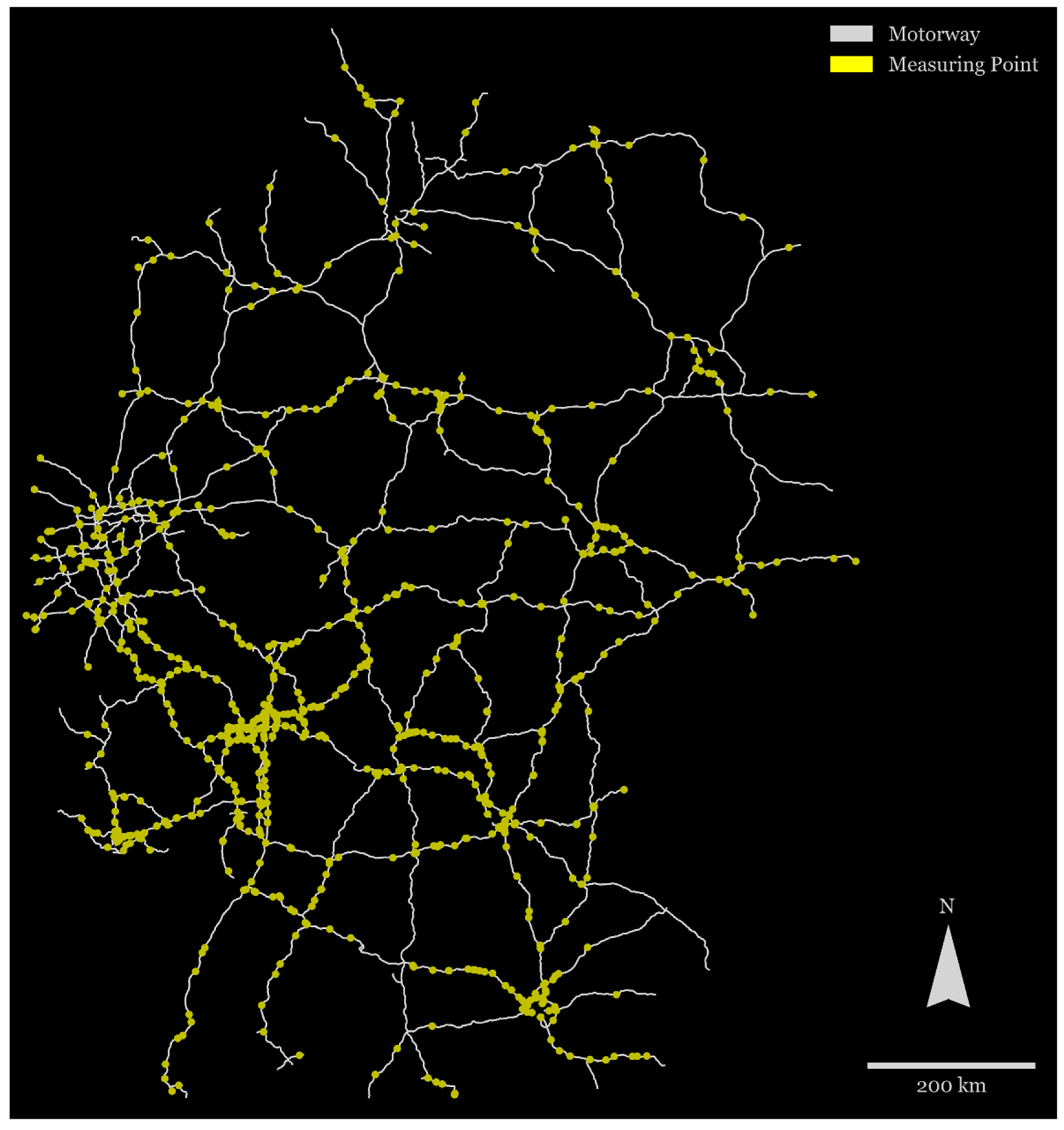
  • The aforementioned information was gathered via measuring points directly installed on individual motorway edges. However, the number of measuring points was very limited. In sequence for the years 2010 to 2014, the number of measuring points that were working as intended and generating data was 80, 102, 108, 114 and 116 points, respectively. Comparing the number of measuring stations to the total motorway network length of 25,665 km, one measuring point had to cover approximately 221 km. Due to this small coverage, relevance of the provided velocity estimations on a large scale is questionable and requires validation.
  • The last argument for an in-depth review of these velocity estimations is one concerning data transparency. The raw data basis as well as the presented estimations have never been published in detail, which inflicts doubts on the credibility of the used methodology and implementation.
Due to the shortcomings of the previously published study by the GEA as well as the general necessity to regularly update such assessments in a perpetually changing field of research [38], the following article aims to validate or disprove political and ecological statements transparently by using publicly available up-to-date data from providers such as OpenStreetMap (OSM) and TomTom. Within our context, publicly available means the source of the information allows access to the information by anyone upon request. We aim to evaluate whether the actual driving speeds as measured by navigation devices throughout the entirety of the road network are as high as presented during previous selected studies based on historical averages. Based on this evaluation, we compute possible savings via the introduction of a speed limit into the network by referencing general emission curves for motorized passenger vehicles. The general research question to be answered via this methodology can therefore be formulated as follows:
How can road networks be enriched by publicly available real-world data to enable CO2 emission calculations?
The remainder of this article is structured as follows: Section 2 describes and applies our methodology to generate representative and routable (road) networks from publicly available data. We begin by retrieving geographical street data via OpenStreetMap to build the network and continue by supplementing the network by means of static, official traffic count and traffic distribution data provided by the GEA. In addition to this static information, we reference and map historically averaged traffic flow information from the TomTom API onto our network to approximate network usage on a per-edge basis throughout any given day. Section 3 continues by outlining the calculations applied to this enhanced network to derive results in terms of CO2 emission reductions achievable by introducing speed limits into the traffic network. Finally, Section 4 discusses the results of our calculations in comparison to the previously published study by the GEA, while Section 5 discusses our findings in relation to previous studies on dynamic traffic speed limits and road participant acceptance in different countries.

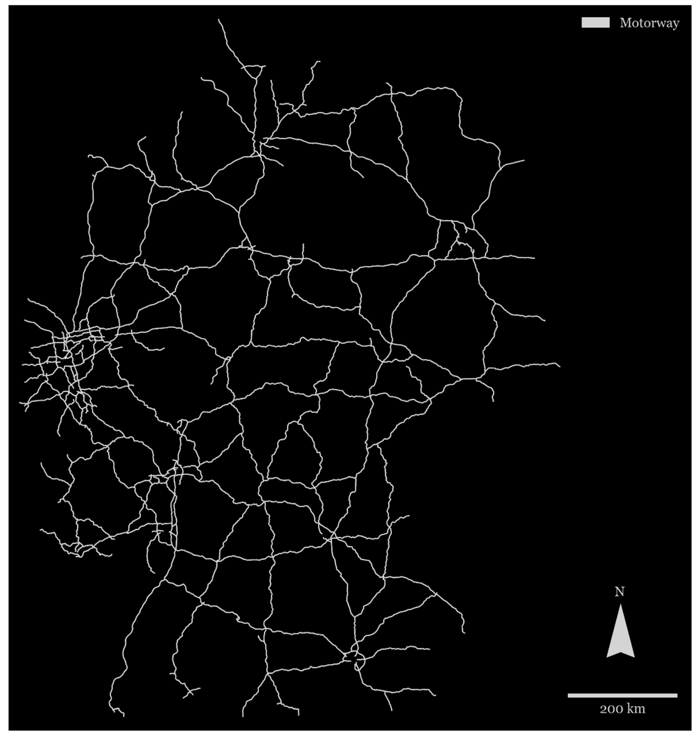
2. Generating Routable Networks from Publicly Available Data

2.1. Extracting Data from OSM

At its core, the methodology to be presented is based on a programmatic analysis of traffic networks. Within this context, a traffic network is defined as a combination of nodes and edges, while edges are defined as a direct link between a set of exactly two nodes. One key component of mapping traffic information onto network data structures is the assumption of directed connections. Therefore, two-way streets are defined by different nodes and edges for each individual direction. This fact plays a crucial role in our need to develop auxiliary functions to correctly map external data onto the right nodes and edges within our network.
Building such networks from scratch would require mapping any relevant street within the network as a connection of nodes and edges while also adding geospatial information to each data point. Due to the sheer size of a country-wide motorway network, this would require hours upon hours of manual and labor-intensive work. This is where open-data platforms like OpenStreetMap come into play. These platforms use crowdsourcing to keep information up to date and openly accessible. Especially for primary road networks, this approach results in a high coverage and accuracy [39,40].
Unsurprisingly, these data pools are used regularly by researchers and practitioners alike to extract detailed topological information. One such framework to create spatial networks from OSM data is the Python package OSMnx by Geoff Boeing [41]. By using this package, we extracted the relevant motorway network, in the example defined via bounding box, and saved the network to disk as a GraphML file. This GraphML file not only contained information about nodes and edges, which, in their sum, define the network, but also included additional information from OSM such as, for example, speed limits as enforced by traffic signs as well as the length in meters for any given edge throughout the network. Note, however, that this information is entirely crowdsourced and might therefore include errors or missing details if no OSM user has added a specific parameter to the platform yet. Nonetheless, this first step left us with a fully connected and routable road network that already contained most basic information. In our context, fully connected and routable describes the fact that the network topology enables the construction of routes from a source to a destination both defined by separate nodes via an uninterrupted path containing several edges. Since every node at least contains information about its geospatial location in the form of latitude–longitude coordinate pairs, we can already visualize the retrieved network as depicted in Figure 1.

2.2. Adding Official Traffic Count Data

We began enhancing the information density of the network by adding traffic count data to identify estimated total quantities of cars on a per-edge basis for any average day. In case of the German motorway network, the “Bundesanstalt für Straßenwesen” (BASt), a governmental institution, regularly measures traffic counts on German primary and secondary roads via a total of 1913 counting points. For application in different countries or regions, corresponding local data sources must be identified accordingly. Of these 1913 counting points throughout Germany, 1125 are located on motorways.
The most recent data available at the time of this writing were from the year 2018. Data was exported as a comma-separated values (.csv) file. It was then imported into the Python workspace where the network resides. By using a getNearestNode function from the OSMnx package with a maximum cutoff radius of 5 km, we mapped the traffic count data (which include latitude/longitude coordinate pairs for every counting point) onto their respective nodes in the network. The contextually relevant information included in this data was comprised of
  • the average daily quantity of cars measured by the counting point,
  • as well as the average daily quantity of trucks measured by the counting point.
After successful mapping, these data were incorporated into the network and could be referenced as a data dictionary for every node’s unique ID. Figure 2 depicts all nodes that now contained traffic data information in yellow.
Since we only mapped data onto the individual closest node identified via getNearestNode, as can be seen in Figure 2, we needed to enrich all remaining nodes throughout our network as well. We achieved this by iterating over all nodes without data and identifying the closest node that contained traffic count data via great-circle distance. Therefore, all nodes around the individual nodes we mapped traffic count data onto were supplied with the same traffic count information. Since our analysis was mostly concerned with actual road sections instead of selective points, we needed to derive a methodology to approximate the traffic count for every edge between two nodes. Throughout multiple iterations of this process, we found that a simple average calculation led to satisfactory and sensible results. Therefore, the formula to estimate the traffic count (TC) for any given edge E defined by one start- and endnode (n1, n2) inside the network is the simple average of both its adjacent nodes. By applying this logic to every edge in the network, we arrived at the first intermediate result of our methodology: A road network enriched by daily traffic count data.
T C E ( n 1 , n 2 ) = 1 2 ( T C n 1 + T C n 2 ) .
As can be seen in Figure 3, throughout Germany, certain areas showed a specifically high traffic count. The western area, mainly the state of North Rhine–Westphalia, as well as the areas around Frankfurt, Stuttgart, Berlin and Munich, depicted a higher-than-average traffic count, which was to be expected since these geographical areas are known socioeconomic conurbations and therefore are central traffic turnstiles throughout the German traffic landscape. Note, however, that by now, the network only contained averaged daily traffic count information for every edge. To perform a thorough and time-specific case study, region-specific car distribution data on an hourly or even a 30-min interval basis needed to be added. Otherwise, all calculations performed within the network would need to be averaged for an entire day. This would require the assumption that traffic was evenly distributed throughout any given day, ignoring the existence of rush hours.

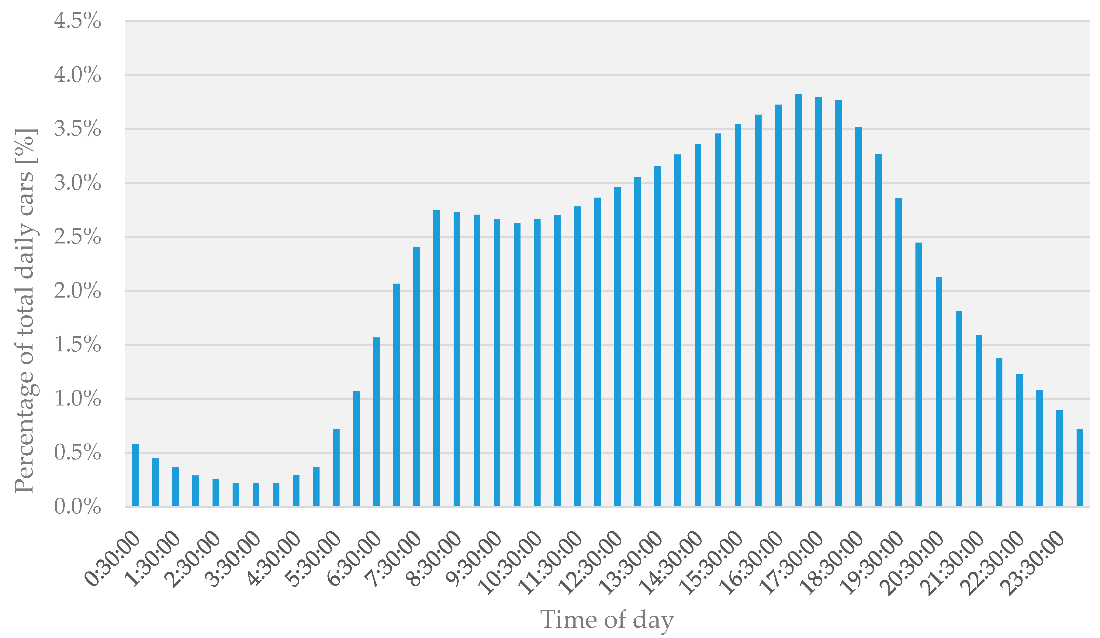
2.3. Adding Additional Traffic Distribution Information throughout the Day

To be able to divide the daily total traffic count per edge into 30-min intervals, a distribution function was derived using another set of officially published BASt data. This second data set is a more detailed version of the previously used traffic count data set and includes hourly data points for the same traffic counting points. We grouped this data by hour and extracted bidirectional traffic counts, derived the average hourly traffic count, and used linear interpolation to approximate data for every half-hour mark. This results in the distribution shown in Figure 4.
As expected, two major peaks were identified, corresponding to the daily commuting rush hours across the German motorway network. At 8:00 a.m., on average, 3% of the total daily number of vehicles were traveling along any given edge. Between 9:00 a.m. and 7:00 p.m., the average percentage of daily vehicles on edge varied between 2.5 and 4%, peaking in between 5:00 p.m. and 6:30 p.m. Between 11 p.m. and 4:00 a.m., only a marginal amount of daily traffic occurred on German motorways. This distribution later allowed for a more precise calculation of flow kilometers across edges for any given timestamp within the network. The total quantity of daily cars per edge (see Section 2.2 and Figure 3) was therefore multiplied by the average percentage from Figure 4. By applying this transformation, specific travel speeds could be weighted by the total sum of applicable flow kilometers. A detailed description of the flow kilometer calculation is given in Section 3.1.
In case no suitable, region-specific data set to estimate a daily traffic distribution is available, the distribution provided in Figure 4 can be used as a reference for countries with comparable size and similar official working hours.

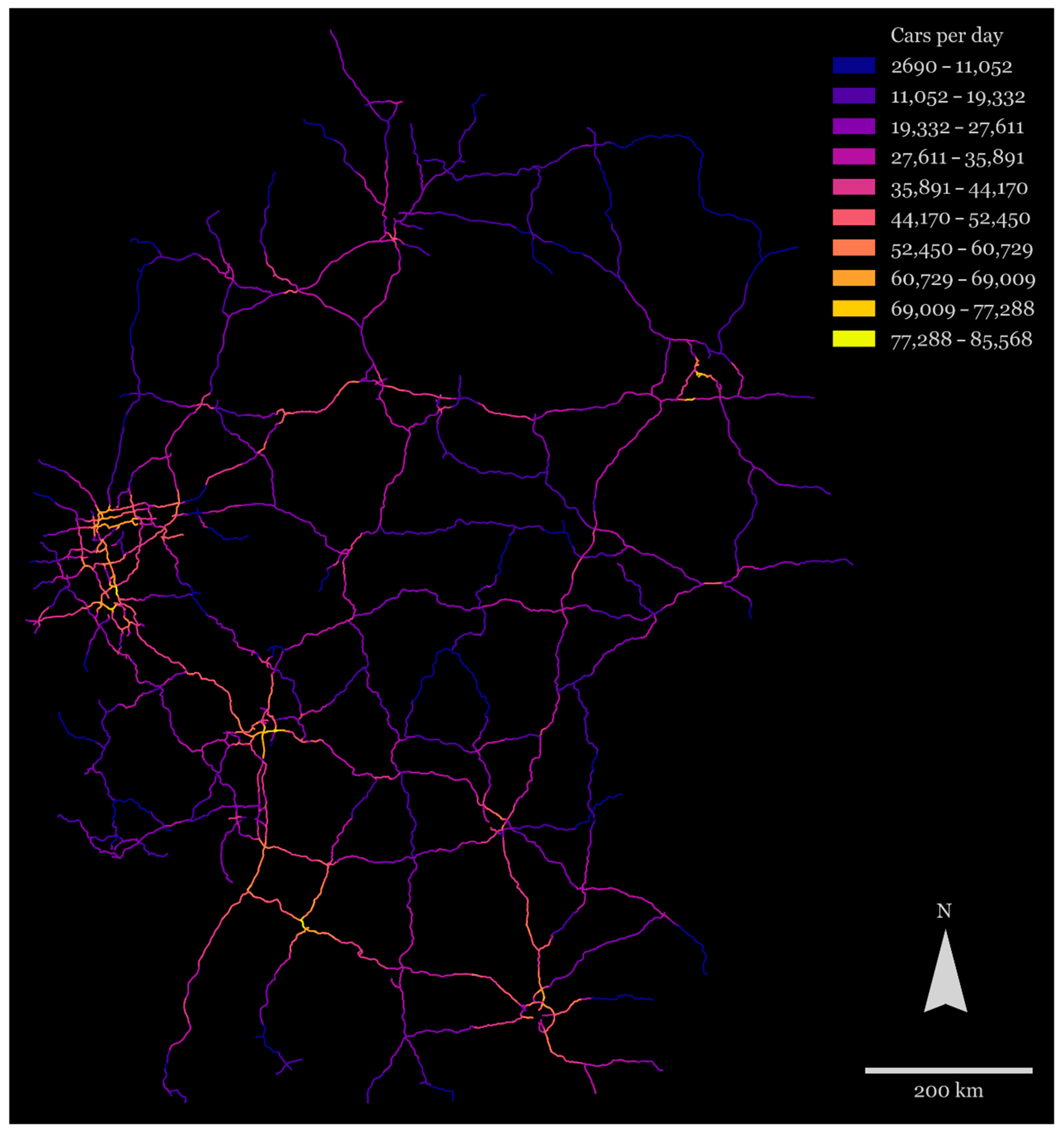
2.4. Adding Real-World Traffic Flow Information to the Network

Continuing, the next part of our methodology was concerned with adding external real-world traffic flow information, in this case using the TomTom Routing Application Programming Interface (API) into the network. Real-world information refers to historical data gathered under practical circumstances, in this case via navigation devices. In comparison, the official (in this case mostly governmental) data sources used in previous studies by the GEA were mostly estimations from small-scale data samples or simulation-based. Therefore, the accuracy of real-world data was considered significantly higher on a wide scale. Data that adhered to this definition could be retrieved programmatically by sending HTTP-compliant GET-requests to a remote API endpoint provided by TomTom. The endpoint allowed access to a database of navigation information supplemented by historical data gathered via personal and commercial navigation devices. Every route request, excluding free quotas provided to experiment with the API, required authentication and incurred a cost. To request and incorporate this data efficiently, we first needed to generate routes such that, at best, every edge included in the network was also included in at least one or more TomTom routing calls while minimizing the total number of routes required.

2.4.1. Generating Network Routes Requestable via TomTom Routing API

A TomTom route is defined by a single source and destination coordinate pair. In between these two points, up to 148 points along the route can be inserted. By trial and error, we devised a five-step process to generate a list of 958 routes in total, which resulted in a network coverage of 98.79% of all relevant motorway nodes. These five steps can be summarized as follows:
  • Identify all motorway endpoints by filtering for network nodes with only one adjacent motorway edge.
  • For every node identified in such a way (destination), apply the Dijkstra algorithm to calculate the shortest path from the network’s central node (source) identified via degree centrality. The result is a sequence of nodes comprising the shortest path.
  • Since the network is defined as a directed graph, Step 1 only handled one direction. Therefore, apply the same logic from Step 1 in reverse to all endpoints that have not yet been found in any route from Step 1.
  • For every remaining endnode, calculate the shortest path from the endnode (source) to the central node (destination).
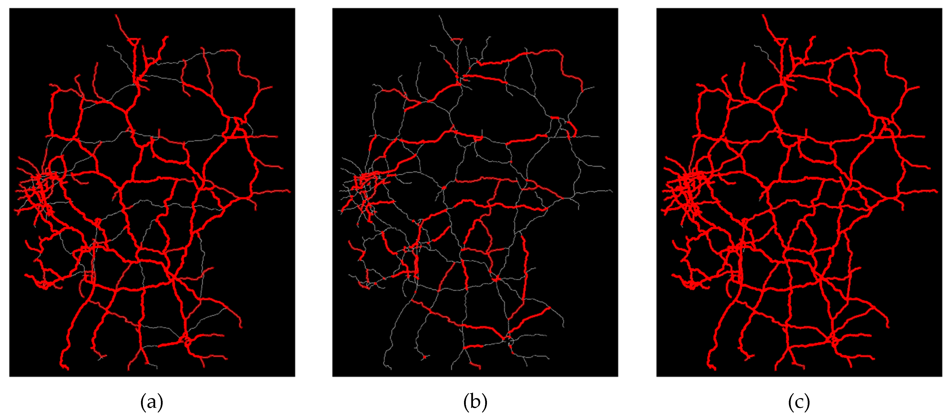
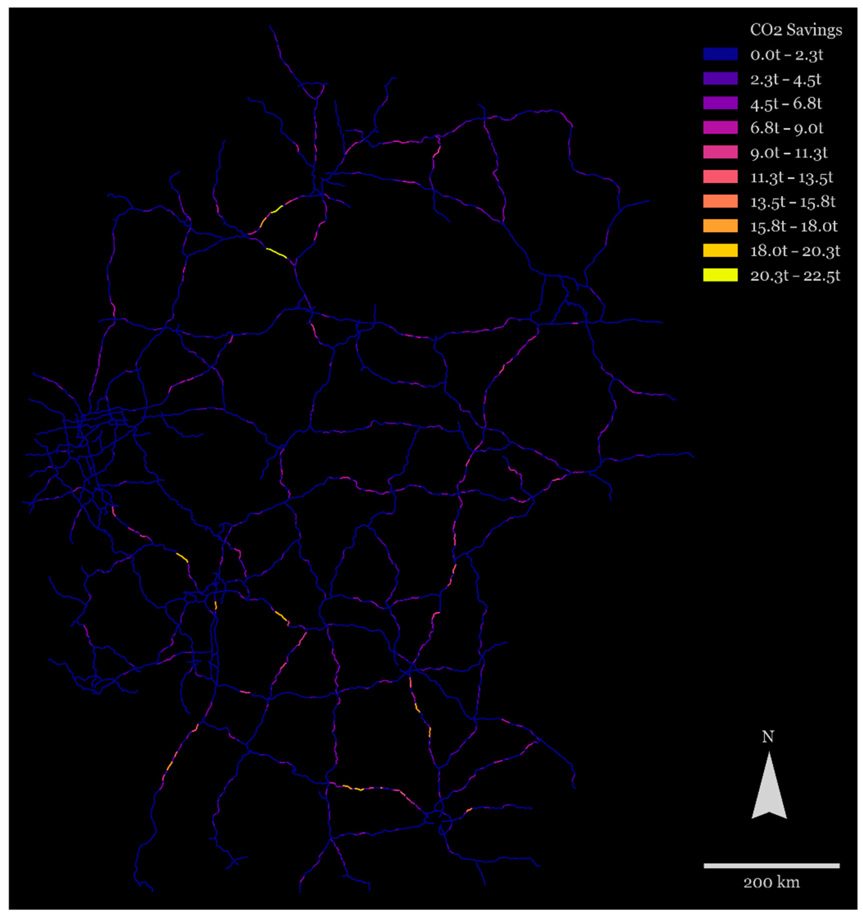
  • After applying Steps 1 and 2, a total of 3630 nodes (out of 13,763 network nodes) were still not included in any path, since these nodes did not lie on any shortest path to or from the previously identified network endpoints in combination with the central node. To handle these nodes as well, we derived the following logic: Select new start- and endpoints within all remaining nodes by identifying nodes that border on exactly one node already included in paths from Steps 1 and 2. For every start- and endnode pairing identified this way, once again create the shortest paths using the Dijkstra algorithm. Figure 5 depicts the different stages of route coverage described above.
As a next step, all 958 routes needed to be converted to a suitable format to use with the TomTom Routing API. In its most basic form, the API requires a route as a colon-delimited list of successive coordinate pairs. We therefore retrieved the latitude and longitude attribute for every node along a route and added them together as a text string in the format.
r o u t e S t r i n g 1   t o   n = l a t 1 : l o n 1 ; l a t 2 : l o n 2 ; ; l a t n : l o n n .
Since the maximum number of points contained within any given TomTom route is restricted to 150, we only added one coordinate pair for every motorway exit along the route, since these exit nodes were the only possible change in direction on a motorway. In case a route contained more than 150 individual points, we divided the full route into individual slices, resulting in multiple API calls for full route coverage. An additional restriction was added in the form of a minimum aerial distance of 100 m between consecutive coordinate pairs. This was incorporated to compensate for slight discrepancies between our network coordinates and TomTom’s routing network, which in the case of high-granularity routing led to mismatches and unwanted detours. The resulting list of routes comprised of coordinate pairings as specified and required for use with the TomTom Routing API was then saved to disk as a .csv file.

2.4.2. Mapping TomTom Routing API Data onto the Network

Using the comma-separated values file created during the previous paragraph, a total of 45,984 API requests were necessary to retrieve all relevant data via the Routing API. The total amount was comprised of 958 requests per individual pass. One pass equaled the request of all routes throughout the network for a single timestamp on any future date, in this case, a future Monday. Requesting a future date led to the calculation of historical averages by TomTom. We observed a timeframe from 0:00 a.m. to 11:30 p.m. in 30-min intervals, leading to 48 separate API passes. One important parameter that must be set is the sectionType = motorway parameter. Using this optional parameter, the TomTom response included additional information describing which of the return legs, corresponding to network edges, lay on the motorway network. This was necessary because, as previously mentioned, the TomTom routing network marginally deviates from the underlying OSM network data. In some cases, this led to TomTom mapping the provided coordinate pairs slightly off to the side of any actual motorway, resulting in high deviations of route length caused by significant detours to navigate to the next freeway ramp and get back on route. Since we did not want to map any of these detours onto our network, we eliminated this problem by using the sectionType parameter.
The result for any individual API call was saved to disk as a JSON file. Every JSON response file contained multiple trip legs. Every leg contained multiple successive coordinate points. Additionally, every leg contained information such as length of the leg in meters, travel time in seconds required to fully traverse the leg, the associated travel speed in kilometers per hour as well as historically averaged counterparts and information about traffic-induced delays. All of these details remained to be incorporated into the local OSM network. To do this, we derived the following logic, which was applied to every response file:
  • Iterate through all legs within the response file;
  • Check if the entirety of points inside a leg are included in a motorway section (meaning the leg is entirely located on a motorway and therefore relevant);
  • If true, calculate the shortest paths from start- to endpoint of the leg within the OSM network, resulting in a list of network nodes along the TomTom leg;
  • If leg length and corresponding OSM network path length deviate by less than 10%, a correct mapping is found;
  • Therefore, iterate across all edges of this path and update the edge attributes with TomTom leg traffic flow information.
By running this logic, we created a data dictionary for every edge contained in the OSM network with a single index for every timestamp during which the edge was traversed by the API response data. This allowed for indexing by specific timestamps and retrieving the average travel speed for any given edge for a specific time of the day.
In total, this methodology reached a traffic flow information coverage across the OSM network of 81.5% of all edges.

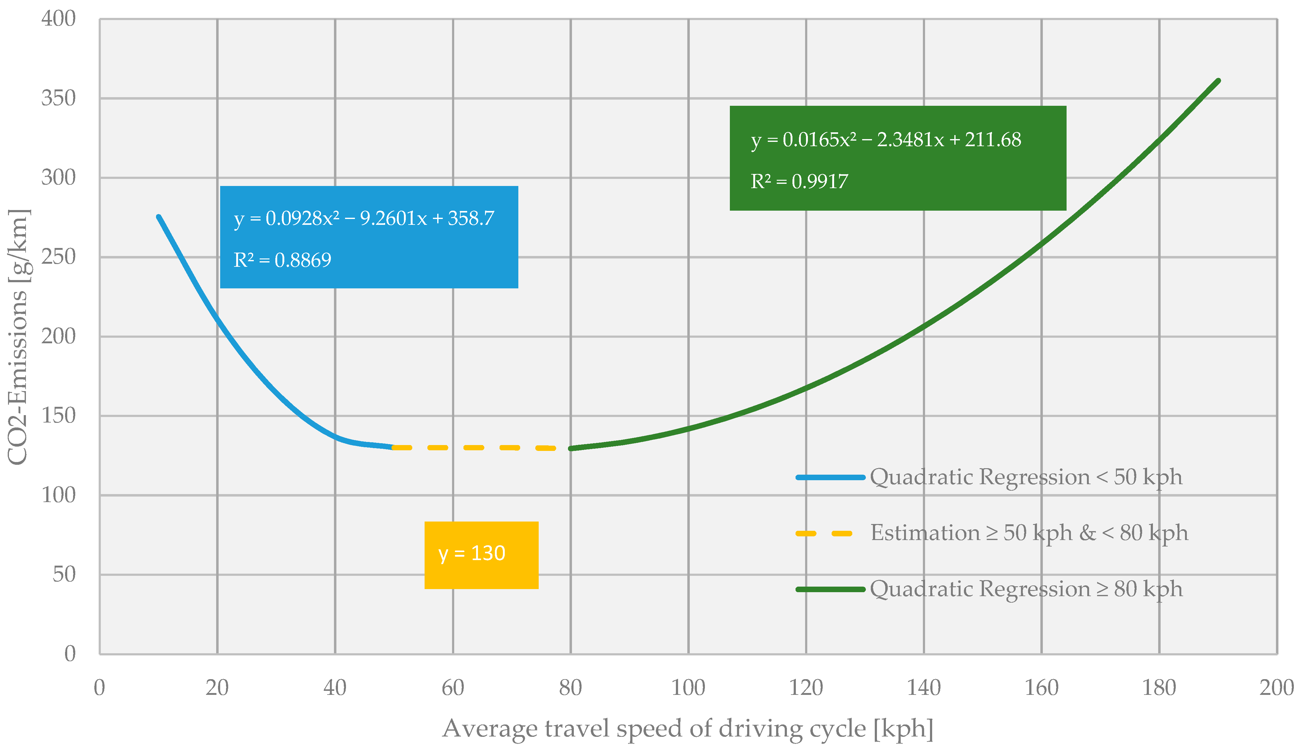
2.5. Translating Average Speed into Estimated Actual Speed

Up to this point, all calculations were based on a single average travel speed for any given edge at a specified time t. Gathering reliable data on travel speed distributions for motorway networks is a laborious task and is, to the best of our knowledge, only undertaken by governmental organizations in small sample sizes. To adjust our calculations, we therefore needed to rely on individually published excerpts of a non-public data set by the GEA. Depicted in Figure 6 is an averaged version of the original speed distribution according to the GEA. By applying this speed distribution to the historically averaged travel speeds returned by TomTom, a more realistic indication of network speeds on any given edge was estimated.

3. Case Study: Calculating CO2 Emissions

The methodology provided in the previous section can be applied to any region that can be defined either via a geographical bounding box or a unique literal identifier like “Bavaria, Germany” to create a programmatically analyzable traffic network as long as general traffic information, OSM and TomTom data are available. The types of analyses possible are predefined solely by the type of additional data that can be gathered. For this case study, we focused on CO2 emission calculations, but the necessary steps can easily be modified to include traffic-induced noise emissions or similar data as well.

3.1. Establishing General Key Parameters for CO2 Calculations

According to the DIN EN 16258:2013-03 norm, every Megajoule of petroleum burned produces 75.2 g of CO2 equivalents (CO2e), while one Megajoule of diesel leads to 71.0 g of CO2e emissions [42]. According to the European Automobile Manufacturers Association, one liter of diesel fuel has an energy density of 36.9 Megajoule, while one liter of petroleum has an energy density of 33.7 Megajoule. Therefore, both engine types produce roughly the same amount of CO2e emission on a per-kilometer basis, depending on the exact composition of the fuel and drivetrain efficiency. Due to this fact, the different fuel types were not analyzed separately.
To quantify the total amount of possible CO2 savings resulting from the introduction of a speed limit, it was necessary to compute the total emissions by any given vehicle in relation to its velocity. As a basis for this calculation, we concurred with the recommendation of the German Environment Agency by referencing adjusted driving cycles provided by the Handbook Emission Factors for Road Transport (HBEFA). For all driving cycles, CO2 emissions on a per-kilometer basis were calculated using the Passenger Car and Heavy-Duty Emission Model (PHEM). For this model, modern Euro-6 passenger vehicles were used as a baseline. Euro-6 vehicles have a nearly identical fleet average of CO2 emissions in day-to-day usage compared to older vehicles adhering to previous Euro-3 to Euro-5 norms [36]. Since more than 90% of registered vehicles in Germany adhered to at least Euro-3 standard and newer, we considered PHEM as representative and generally applicable for this analysis. Since most emission models, PHEM included, are only defined for velocities up to 130 kph, the GEA provides unpublished “further driving cycles” up to 190 kph inside their study, which we could neither validate nor disprove but adhered to for comparability between both studies. Figure 7 depicts the final regression model used to estimate CO2 emissions by means of averaged travel speeds.
Applying this regression to all edges within the network resulted in the total amount of CO2 g emitted on any average Monday throughout the German motorway network. Unfortunately, this result only held true under the previous assumption that all traffic is evenly distributed across the day. It was therefore prone to error because travel speeds as well as traffic delays vary throughout the day, as can be measured by inspecting the specific attributes across edges throughout the day. Given the fact that during a possible morning rush hour, the travel speed on a specific edge is much lower than during the rest of the day, this should be weighted accordingly by also including the percentage of daily cars that need to traverse the edge at this specific time of the day into the calculation (see Section 2.3).
The measurement of kilometers traveled along an edge multiplied by the number of total applicable cars at any specific time t was therefore defined as the edge flow kilometers of any edge at time t. Due to this, the total edge flow kilometers (TEFK) of any edge can be calculated via the formula
T E F K = t = 1 48 e d g e   l e n g t h   [ m ] 1000 ( P e r c e n t a g e   o f   d a i l y   c a r s ( t ) T C E ) ,
which enables weighting of time-specific edge calculations based on their proportion of total edge flow kilometers. All following calculations and results depicted were based on these weighted flow kilometers.

3.2. Applying Speed Limits to the Network

Introducing a speed limit into the network was as simple as defining a cutoff-threshold that was applied at time of calculation. During unrestricted state, every network edge contained several average travel speeds—one value per timestamp. By defining an exemplary threshold of 120 kph, we simply cut off any average travel speeds above 120 kph on a per-unrestricted-edge basis. Any edge with a speed below the threshold remained unchanged while sections above the threshold were limited to the threshold when included in any calculation. This simplified introduction of a speed limit could therefore be compared to the introduction of legally binding, static traffic signs on the motorway network. As depicted in Figure 6, not all network participants could be expected to implicitly comply with the legal restrictions. Therefore, we additionally applied the speed distribution in restricted state (see Figure 6, depicted in blue) to arrive at a more realistic speed distribution for any given edge at specified time t. A thorough discussion of the results achieved by introducing different speed thresholds into the network can be found in the upcoming section.

4. Results

In this section, we examine the results presented by the German Environment Agency within the official study and compare these results to calculations derived directly via the network.

4.1. Network Benchmark

We began by comparing basic statements concerning the general motorway infrastructure, its state of restriction and general usage-patterns to establish a baseline similarity between both the official study and our programmatical analysis. The results of this comparison are shown in Table 1.
According to the GEA, 55.5% of the German motorway flow across the network currently has no permanent speed restriction (e.g., static traffic signs) in place. In cases of no speed restriction, hereby defined as “open” sections, the average travel speed across network participants is measured at 124.7 kph. A total of 10.95% of network flow is permanently restricted to 100 kph with a measured average travel speed of 103.3 kph. The largest part of the restricted network flow is statically restricted to 120 kph with an average travel speed slightly below the allowed maximum speed at 115.6 kph. Another 7.4% of network flow is presented as currently restricted to 130 kph with an average travel speed of 118.3 kph. The remaining 8.9% of network flow belongs to speed categories below 100 kph, as is the case with inner-city motorways or permanent construction sites. On average, travel speed across all network flow is 116.5 kph, according to the GEA.
By retrieving the same statistics programmatically via the motorway network, we arrived at comparable results for speed restrictions of 100 kph, 130 kph and for non-restricted traffic flow with 8.38% and 102.9 kph, 8.8% and 118.82 kph as well as 53.5% and 126.77 kph, respectively. In the case of network flow permanently restricted to 120 km, our results differed significantly from the official study. The network analysis resulted in 25% of flow kilometers that were currently restricted to 120 kph instead of the previously cited 17.2%. In terms of average speed on these sections, the results converged again with the network analysis, resulting in 114.24 kph compared to 115.6 kph. This difference was most likely caused by including versus omitting dynamic traffic signs during the analysis. While we have no specific information on how dynamic traffic signs were handled by the GEA, our network defaulted to assuming an average restriction of 120 kph. Across all flow kilometers, the network calculated an average travel speed of 119.37 kph.

4.2. Theoretical versus Practical Speed Restrictions

By definition, a restriction only occurs if the historically averaged travel speed is higher than the threshold at which the speed limit would occur. This means that it is entirely possible that even though a particular section of the motorway network legally allows for a maximum speed of 130 kph, meaning that it would in theory be restricted by a speed threshold of 120 kph, in reality the historically achieved travel speed averages at about 118 kph. What this in turn means is that even though on first glance, a road previously limited to 130 kph might be restricted by a general speed limit, in reality most network participants on this road section are never able to reach travel speeds above the speed limit throughout most of the day, meaning the restriction would not affect them at all but would also not contribute to any CO2 savings resulting from a general speed limit. While critics of general speed restrictions base their argumentation of heavy incursions on personal freedom on the first aspect of currently allowed maximum speed limits, the more relevant aspect in terms of CO2 reductions is the analysis of practical, real-world facts as recorded by navigation devices.
Putting these claims to the test by adding the previously retrieved historical traffic details from TomTom into the equation, our network analysis revealed that only 7.19% of all flow kilometers allow for high-speed driving. High-speed driving is defined as the circumstance that a road section is currently not restricted by any traffic signs (“unrestricted” or “open”) and has no traffic-induced delays, for example, caused by traffic jams or construction sites. Comparing this 7.19% of practically “unlimited” flow kilometers according to real-world TomTom data (where it is indeed possible to achieve high speeds in day-to-day driving) to the previously described 53.5% of theoretically unrestricted flow according to traffic signs, a major gap between theory and practice became obvious.
Additionally, a total of 65.61% of all flow kilometers on average do not reach their legally allowed travel speed (according to traffic signs) due to general traffic volume as well as traffic jams. To put it simply, most motorway sections operate at suboptimal performance due to traffic delays induced by too many network participants simultaneously claiming usage of the same finite infrastructure. Additionally, another 1.61% of all flow kilometers operate below their legally allowed speed limits without any traffic-induced delays at all. On the other hand, for 22.5% of flow kilometers, the average daily travel speed exceeds the legally allowed speed limit, leading to illegal speeding on certain motorway sections. It therefore appears that major reductions in CO2 emissions can already be achieved by enforcing current speed limitations more strictly.
Referencing the speed limit of 120 kph as proposed by the GEA, the introduction of such a general speed limit across the entire network would restrict 50.74% of practical flow kilometers, leading to a decrease in average speed of 4.1 kph or 2.94% compared to the status quo.

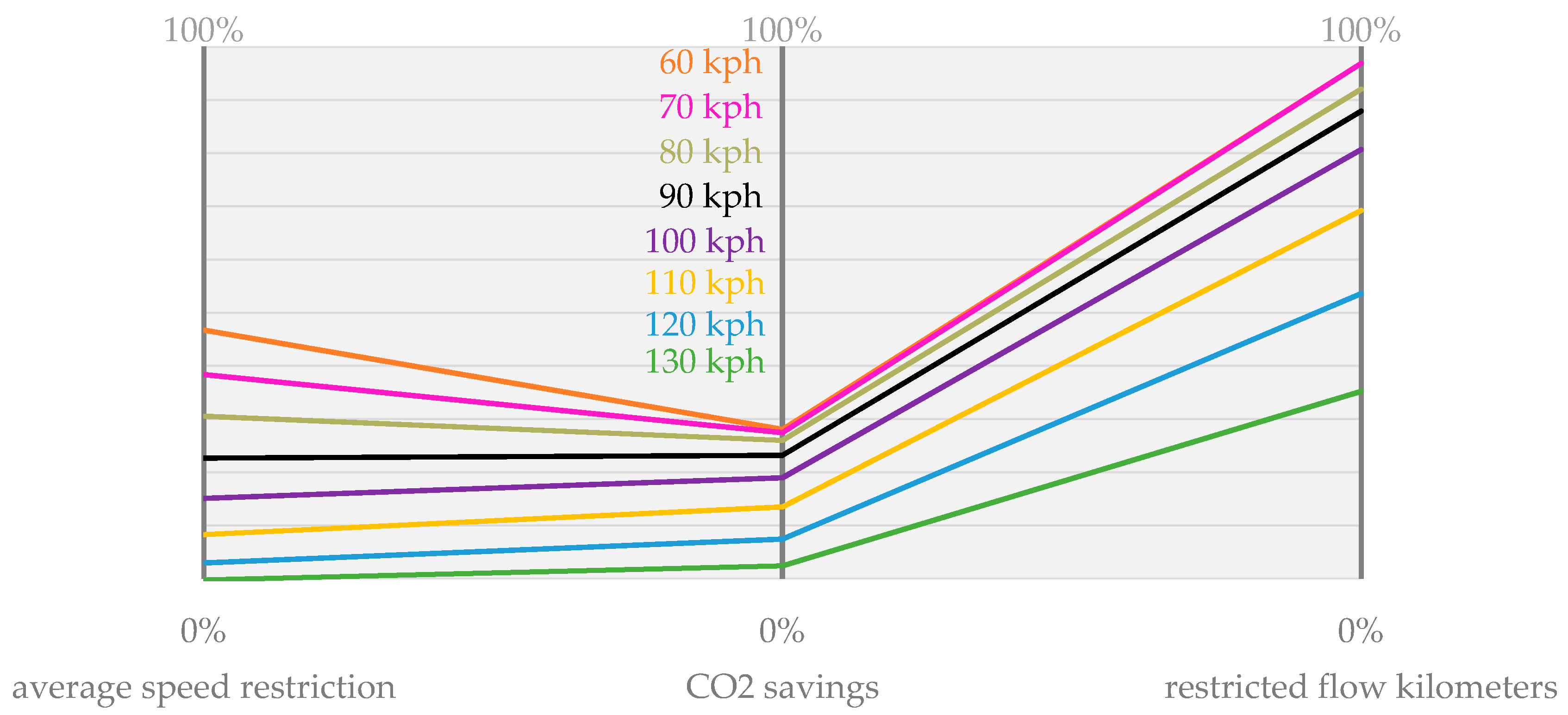
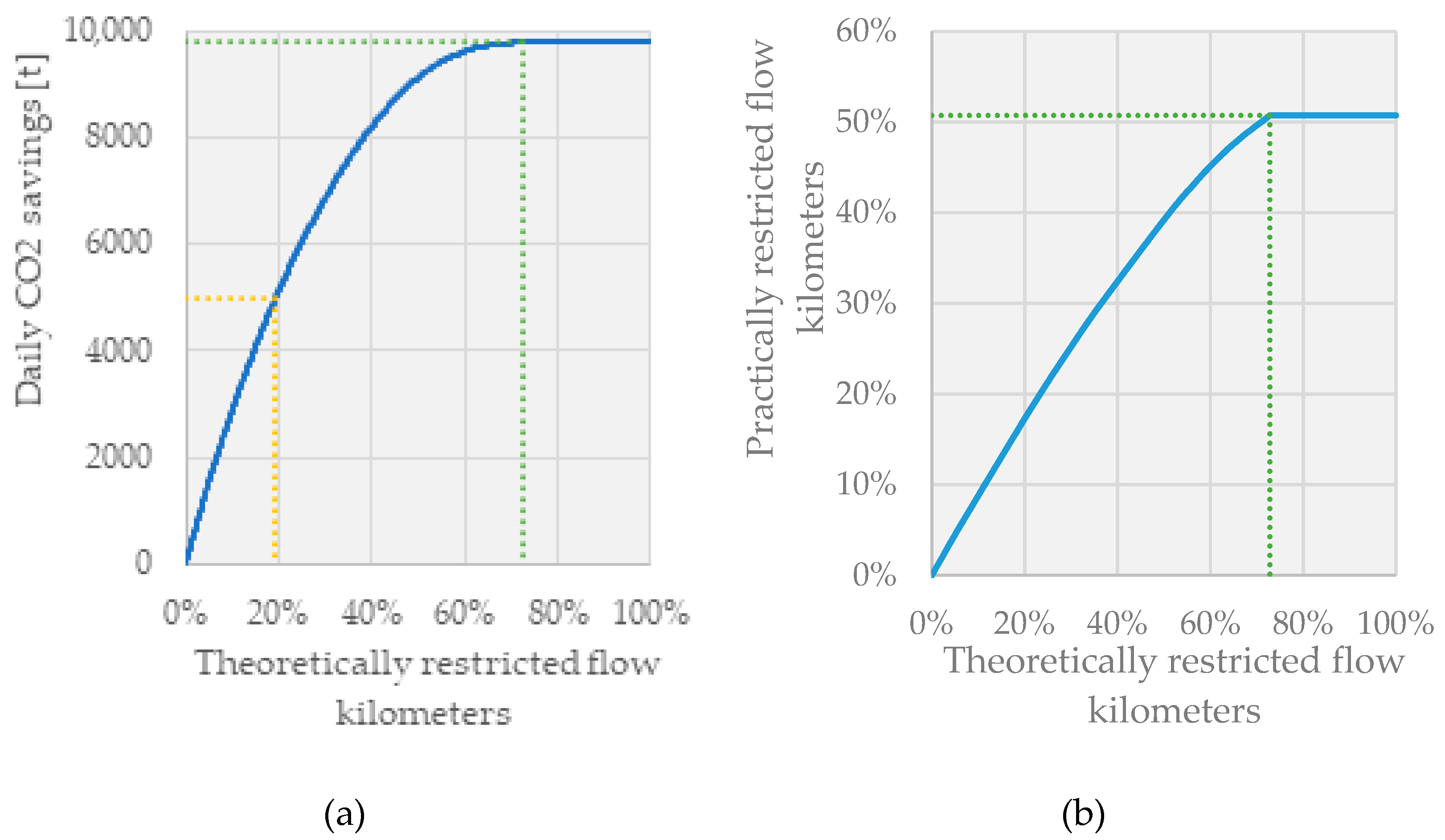
4.3. Analysis of Possible CO2 Reductions by Inducing Speed Limits

Now that we have established that a general speed limit of 120 kph across all German motorways would restrict 50.74% of total daily flow kilometers based on real-world traffic data, the question remains as to what proportions of CO2 emission savings would result from such measures.
During the second major part of the analysis, we identified potential emission savings on a per-edge basis by calculating the total CO2 emissions with and without a speed limit threshold in place. To achieve this, we calculated CO2 emissions by inserting the historical travel speeds as measured by TomTom, adjusted by applying the travel speed distribution previously depicted in Figure 6 into the regression model and retrieved the respective CO2 emissions. If the historic travel speed was higher than the introduced speed threshold, the value of the threshold was inserted instead. According to our traffic data network coverage of 81.5%, we scaled up the results of our calculations by dividing each absolute CO2 value by.815, such that the remaining 18.5% of network edges not covered by any TomTom data were likewise included within the results to be presented.
By applying this logic to the network, total daily CO2 savings of 7.43% compared to the unrestricted network can be achieved, while the aforementioned 50.74% of flow kilometers throughout the German motorway network would practically be restricted. In absolute measures, this would save 9796.37 tons of CO2 emission per day or 3,575,675.95 tons of CO2 per year within the transport sector. To calculate yearly savings, we assumed a historically averaged Monday is representative for any given weekday. Future research might focus on analyzing network characteristics depending on different days of the week, especially Monday to Friday versus the weekend.
The same procedure was carried out for several different thresholds ranging from 60 kph to 130 kph, comparing potential CO2 savings to network restrictions necessary to achieve these savings. The results are shown in Table 2.
One interesting result from Table 2 is the fact that a speed limit of 130 kph would result in a negative change of average speed (meaning an average speed increase) throughout the network. On first sight, this appears to be counterintuitive. Nonetheless, these results are a good indicator for the underlying assumption that the introduction of a speed limit would implicitly result in road participants adhering to these new regulations. Due to the previously described average speed throughout the network of 119.38 km an hour, adhering to the speed limit would require the general road user to increase their average driving speed. Since the current average network travel speed results not only from driver preference but also primarily from infrastructural performance of the network in general, it is highly unlikely that such a broad change could be realized.
To allow for a representative comparison between both studies it was important to keep in mind that while the GEA cited the total amount of CO2 emitted by motorized vehicles as 44.5 million tons annually, a calculation within our network returned a total of 48.12 million tons, based on official and supplemented traffic count information as well as navigation service provider data. Therefore, percentage-wise comparison required normalization as provided within Table 3.
The estimated CO2 savings for a targeted speed limit of 120 kph differed by 1.57 percentage points, based on the absolute difference of 700,000 tons annually between our analysis and the results presented by the GEA. This gap is a direct result of the different methodologies applied. While the GEA used a fixed set of measuring points to extrapolate traffic flow information across the network, the methodology presented in this article referenced real-world traffic data provided by navigation devices across 81% of the network. Results differed more significantly for the remaining two cases of 100 and 130 kph. These variations stemmed from the fact that Löhe [37], the major data source for the GEA analysis, only provides data from measuring points for restricted sections with a speed limit of 120 kph. Therefore, the GEA was only able to provide general estimations for scenarios of 100 and 130 kph, while our data-driven methodology could draw from broad navigation service provider data to estimate a more realistic speed distribution for these additional thresholds.

4.4. On the Way to Well-Chosen Speed Limits

While the goal of minimizing CO2 emission is generally accepted as beneficial, discussions on the dimensions of restrictions necessary and acceptable to achieve these savings continue. To better compare the proportions of restrictions necessary for achievable CO2 savings, the parallel coordinate plot in Figure 8 is used.
A completely parallel line in Figure 8 equates to a directly proportional relation between two parameters. An example for this is the left-hand side for a speed limit of 90 km (black line). To achieve percentage-based CO2 savings of 23.16% compared to the unrestricted network state, the average speed across the network must be reduced by 22.66%. In contrast to that, a steeper line in any direction (upward or downward slope) indicates a non-proportional relation between two attributes. The steeper the line, the more disproportional the relation is. Coming back to the major example of this article, the blue line indicates a speed limit of 120 km per hour. While the left-hand side relation between the average speed to be restricted and the potential savings is a positive one (an average speed reduction of 2.94% results in average daily CO2 savings of 7.43%), the right-hand side supports claims of disproportionate incisions as 50.74% of total flow kilometers would require restrictions to achieve this 7.43% of CO2 savings. The same can be said for any of the other thresholds considered during this case study.
To seek a mutually acceptable compromise for both parties—supporters and opponents of general speed restrictions—we took a closer look at the 120 kph restriction. In the case of 120 kph, 50.74% of traffic flow would practically be restricted. The total CO2 emissions could be reduced by 7.43%, equaling 9796.37 tons per day. Figure 9 indicates the consequences of partial restrictions. The street sections have been ordered by the corresponding percentage of reduced CO2 emissions in the case of a 120 kph restriction. A restriction of the top 19% of street sections in terms of percentage of CO2 savings would lead to absolute CO2 savings of 5000 tons daily, which equals about 50% of total possible savings considering a speed limit of 120 kph.
One fact worth mentioning while examining Figure 9 is the plateau value at approximately 72% of cumulated flow regulated by traffic signs, whereas our previous calculations showed a maximum restriction of 50.74% of flow kilometers. This stems from the fact that the conceptualized restrictions we applied to the network would be time-independent via the introduction of static and permanent speed signs on road sections, but the level of speed and therefore the classification of whether specific flow kilometers within the network will be restricted or not are highly time-dependent. In fact, a high amount of flow would theoretically be regulated by traffic signs, but in practice would not reach the threshold of 120 kph (i.e., originally unrestricted flow at rush hours). This suggests establishing dynamic traffic signs to adjust speed limits throughout different times of the day, based on actual traffic volume at specified time t. Therefore, the x-axis of Figure 9 indicates the flow that is driven on edges with potential speed signs, but its practical restriction depends on the daytime-specific actual driving speeds. As a result, the amount of flow kilometers that are theoretically restricted is higher than the amount of flow kilometers that are practically restricted. This is worth mentioning since speed limit opponents will argue based on a 72% restriction extracted from Figure 9, which in fact distorts the proportion of restricted flow kilometers and ignores dynamic real-world conditions. A more in-depth analysis and discussion on the topic of dynamic traffic regulation can be found in the upcoming section.
Figure 10 depicts the result in terms of absolute CO2 savings per network edge (with an average edge length of 1.8 km) throughout the German motorway network according to our network analysis. Unsurprisingly, the highest savings are to be found on motorway edges in between large cities. As proximity to city centers increases, only marginal savings, if any, exist, which is to be expected since most of the traffic converges at these network intersections before it splits into different directions. Therefore, these highly used parts of the network predominately suffer from traffic jams, decreasing the historically averaged travel speed. Due to this decrease in average travel speed, most motorways located in close proximity to major cities are not affected by a speed limit since their default travel speed is already below the maximum speed allowed via the introduction of a speed threshold, resulting in no noteworthy CO2 savings on these network edges.

5. Discussion

Our results verify the assumption that a general speed limit throughout the German motorway network can help reduce the annual amount of CO2 emission by reducing average travel speeds. The range of achievable savings calculated using our proposed methodology is in line with previous governmental studies by the German Environment Agency as well as the body of literature on this topic [24,28,30,36].
The methodology presented in this paper delivers a coherent guide on how to programmatically leverage official governmental data, historical traffic information as well as open-data platforms to improve on many of the shortcomings of previous studies, mainly on the issue of non-published data sets as well as the lack of transparency and reproducibility caused by it.
As discussed in Section 4, it is not necessary to apply speed limits to the whole network. Instead of this, we suggest the usage of so-called Variable Speed Limits (VSL). In addition to reducing the obstacle of perceived justification, VSL contribute significant further side effects, mainly flow optimization, reduced travel times, a decrease in traffic shock waves as well as an increase in road safety in general [43,44,45,46,47,48,49,50].
Unfortunately, motorists generally do not adhere to speed limits [51]. Because of that, VSL still require enforcement to realize many of their implied benefits [52,53,54], which results in high upfront and maintenance costs. It is therefore necessary to precisely evaluate the benefits resulting from these investments. In our case, Section 3 and Section 4 focused on environmental benefits in terms of CO2 emission savings. The calculated savings of 3.6 million tons annually (by implementing a speed limit of 120 kph) would require 50.74% of daily flow kilometers to be restricted throughout the network. However, this estimation resides on the lower end of the spectrum since it currently neglects the positive impacts of VSL previously described. Due to this, a wide-scale implementation of Variable Speed Limits could lead to reduced road occupancy, resulting in a smoothed traffic flow, which transfers to better driving patterns that require less acceleration and braking throughout a journey, decreasing the fuel consumption of any given vehicle, which directly correlates to fewer fossil fuels burned and less CO2 emitted throughout the network.
Unfortunately, the proposed introduction of VSL into the network highlights a major limitation of our methodology, since these effects cannot currently be determined because we adhered to simplifications and assumptions provided by the GEA for the sake of comparability. Due to this, future research might focus on improving on these assumptions and supplementing the network via more specific and scientifically verifiable calculations. Some key points to be approved upon can therefore be summarized as follows:
We adopted the average-based CO2 emission functions derived by the GEA. Since data on how the underlying driving cycles have been calculated are non-public, we suggest building transparent CO2 emission functions. To achieve this, vehicle registration data can be analyzed to extract the distribution of different vehicle types moving on German motorways. In addition to that, open access frameworks like COPERT could be utilized to differentiate CO2 emission curves by vehicle and fuel type [55]. The biggest issue that needs addressing is the fact that CO2 emission functions often have a limited definition range. COPERT functions are currently only defined up to velocities of 130 kph. Therefore, one crucial part is finding or developing emission functions that adhere to the following two requirements: (1) they should be detailed enough to differentiate between vehicle and fuel types, and (2) must be robust at higher speeds, which are driven on legally unrestricted motorways.
Additionally, the applicability and reliability of the traffic distribution functions provided by the GEA depicted in Figure 6 require further validation. Since the introduction of a general speed limit might significantly impact the driving patterns throughout the network, leading to increased travel times and longer lengths of stay within the network, future studies could focus on a simulation-based approach to validate the assumed distribution functions and their impact on network-wide CO2 emission savings. Microscopic traffic simulation would also allow for the inclusion of VSL-based calculations [56,57,58], drastically improving on the applicability of our methodology to practical debates and potentially offsetting concerns on the topic of negative changes in driving patterns.

6. Conclusions

The contribution of this paper is a methodology to allow for transparent data analysis in road networks by enriching OpenStreetMap (OSM) data with publicly available traffic information on a dynamic scale.
We apply our methodology to contribute to the discussion of possible CO2 emission savings via the introduction of a speed limit to the German motorway network by comparing our programmatical results to the official study by the German Environment Agency published in 2020. The comparison reveals that while the key facts and estimations in terms of network infrastructure as presented by the GEA hold true, major differences between the theoretical assumptions of network performance in terms of possible travel speeds and practical data gathered by navigation service providers can be identified.
We have quantified and shown that the introduction of a flat-rate speed limit of 120 km per hour would result in a theoretical restriction of about 70% of total flow kilometers across the German motorway network, saving 3,575,675.95 tons of annual CO2 emissions within the transport sector. More importantly, we quantify that nearly 100% of these savings could already be realized by restricting only 50.74% of all network sections dynamically throughout the day due to significant variations in time-dependent road utilization. Additional calculations for speed limits from 60 kph to 130 kph were provided as a means of sensitivity analysis to our findings.
Since we adopted multiple simplifying assumptions provided by the GEA for sake of comparability, future research might focus on speed distribution patterns in the context of 100 and 130 kph as well as on validating the presented driving cycles to calculate the speed-induced CO2 emissions. In addition to that, the influence of Variable Speed Limits on traffic flow smoothness and its consequences, such as the level of CO2 emissions and the probability of accidents, are currently not included and should be analyzed in detail.

Author Contributions

Conceptualization, J.K. and M.B.; methodology, J.K. and M.B.; software, J.K. and M.B.; validation, J.K. and M.B.; writing—original draft preparation, J.K.; writing—review and editing, M.B.; visualization, M.B. and J.K.; project administration, J.K.; supervision, F.K. All authors have read and agreed to the published version of the manuscript.

Funding

This research received no external funding.

Data Availability Statement

Data available in a publicly accessible repository.

Conflicts of Interest

The authors declare no conflict of interest.

References

  1. Kuramochi, T.; Roelfsema, M.; Hsu, A.; Lui, S.; Weinfurter, A.; Chan, S.; Hale, T.; Clapper, A.; Chang, A.; Höhne, N. Beyond national climate action: The impact of region, city, and business commitments on global greenhouse gas emissions. Clim. Policy 2020, 20, 275–291. [Google Scholar] [CrossRef] [Green Version]
  2. Manne, A.; Richels, R. The Greenhouse Debate: Econonmic Efficiency, Burden Sharing and Hedging Strategies. Energy J. 1995, 16. [Google Scholar] [CrossRef]
  3. Woensel, T.; Creten, R.; Vandaele, N. Managing the environmental externalities of traffic logistics: The issue of emissions. Prod. Oper. Manag. 2001, 10, 207–223. [Google Scholar] [CrossRef] [Green Version]
  4. Kellner, F. Exploring the impact of traffic congestion on CO2 emissions in freight distribution networks. Logist. Res. 2016, 9. [Google Scholar] [CrossRef] [Green Version]
  5. Durbin, T.D.; Johnson, K.; Miller, J.W.; Maldonado, H.; Chernich, D. Emissions from heavy-duty vehicles under actual on-road driving conditions. Atmos. Environ. 2008, 42, 4812–4821. [Google Scholar] [CrossRef]
  6. Santos, G. Road transport and CO2 emissions: What are the challenges? Transp. Policy 2017, 59, 71–74. [Google Scholar] [CrossRef]
  7. Liang, Y.; Niu, D.; Wang, H.; Li, Y. Factors Affecting Transportation Sector CO2 Emissions Growth in China: An LMDI Decomposition Analysis. Sustainability 2017, 9, 1730. [Google Scholar] [CrossRef] [Green Version]
  8. Klumpp, M. To Green or Not to Green: A Political, Economic and Social Analysis for the Past Failure of Green Logistics. Sustainability 2016, 8, 441. [Google Scholar] [CrossRef] [Green Version]
  9. Hickman, R.; Banister, D. Looking over the horizon: Transport and reduced CO2 emissions in the UK by 2030. Transp. Policy 2007, 14, 377–387. [Google Scholar] [CrossRef]
  10. Haas, T.; Sander, H. Decarbonizing Transport in the European Union: Emission Performance Standards and the Perspectives for a European Green Deal. Sustainability 2020, 12, 8381. [Google Scholar] [CrossRef]
  11. Lajunen, A.; Kivekäs, K.; Vepsäläinen, J.; Tammi, K. Influence of Increasing Electrification of Passenger Vehicle Fleet on Carbon Dioxide Emissions in Finland. Sustainability 2020, 12, 5032. [Google Scholar] [CrossRef]
  12. Rietmann, N.; Hügler, B.; Lieven, T. Forecasting the trajectory of electric vehicle sales and the consequences for worldwide CO2 emissions. J. Clean. Prod. 2020, 261, 121038. [Google Scholar] [CrossRef]
  13. Bienias, K.; Kowalska-Pyzalska, A.; Ramsey, D. What do people think about electric vehicles? An initial study of the opinions of car purchasers in Poland. Energy Rep. 2020, 6, 267–273. [Google Scholar] [CrossRef]
  14. Kapustin, N.O.; Grushevenko, D.A. Long-term electric vehicles outlook and their potential impact on electric grid. Energy Policy 2020, 137, 111103. [Google Scholar] [CrossRef]
  15. Funke, S.Á.; Sprei, F.; Gnann, T.; Plötz, P. How much charging infrastructure do electric vehicles need? A review of the evidence and international comparison. Transp. Res. Part D Transp. Environ. 2019, 77, 224–242. [Google Scholar] [CrossRef]
  16. Greene, D.L.; Kontou, E.; Borlaug, B.; Brooker, A.; Muratori, M. Public charging infrastructure for plug-in electric vehicles: What is it worth? Transp. Res. Part D Transp. Environ. 2020, 78, 102182. [Google Scholar] [CrossRef]
  17. Fridstrøm, L. Who will bell the cat? On the environmental and sustainability risks of electric vehicles: A comment. Transp. Res. Part A Policy Pract. 2020, 135, 354–357. [Google Scholar] [CrossRef]
  18. Kawamoto, R.; Mochizuki, H.; Moriguchi, Y.; Nakano, T.; Motohashi, M.; Sakai, Y.; Inaba, A. Estimation of CO2 Emissions of Internal Combustion Engine Vehicle and Battery Electric Vehicle Using LCA. Sustainability 2019, 11, 2690. [Google Scholar] [CrossRef] [Green Version]
  19. Ram, M.; Child, M.; Aghahosseini, A.; Bogdanov, D.; Lohrmann, A.; Breyer, C. A comparative analysis of electricity generation costs from renewable, fossil fuel and nuclear sources in G20 countries for the period 2015-2030. J. Clean. Prod. 2018, 199, 687–704. [Google Scholar] [CrossRef]
  20. Canals Casals, L.; Martinez-Laserna, E.; Amante García, B.; Nieto, N. Sustainability analysis of the electric vehicle use in Europe for CO2 emissions reduction. J. Clean. Prod. 2016, 127, 425–437. [Google Scholar] [CrossRef]
  21. Shirazinejad, R.S.; Dissanayake, S. Speed Characteristics in Relation to Speed Limit Increase and Its Influence on Driver’s Speed Selection Behavior. Sustainability 2020, 12, 1369. [Google Scholar] [CrossRef] [Green Version]
  22. Yang, J.; Xu, J.; Gao, C.; Bai, G.; Xie, L.; Li, M. Modeling of the Relationship Between Speed Limit and Characteristic Speed of Expressway Traffic Flow. Sustainability 2019, 11, 4621. [Google Scholar] [CrossRef] [Green Version]
  23. Fergusson, M. The effect of vehicle speeds on emissions. Energy Policy 1994, 22, 103–106. [Google Scholar] [CrossRef]
  24. Keller, J.; Andreani-Aksoyoglu, S.; Tinguely, M.; Flemming, J.; Heldstab, J.; Keller, M.; Zbinden, R.; Prevot, A.S.H. The impact of reducing the maximum speed limit on motorways in Switzerland to 80km h−1 on emissions and peak ozone. Environ. Model. Softw. 2008, 23, 322–332. [Google Scholar] [CrossRef]
  25. Frey, H.C.; Rouphail, N.M.; Zhai, H. Speed- and Facility-Specific Emission Estimates for On-Road Light-Duty Vehicles on the Basis of Real-World Speed Profiles. Transp. Res. Rec. J. Transp. Res. Board 2006, 1987, 128–137. [Google Scholar] [CrossRef]
  26. Lejri, D.; Can, A.; Schiper, N.; Leclercq, L. Accounting for traffic speed dynamics when calculating COPERT and PHEM pollutant emissions at the urban scale. Transp. Res. Part D Transp. Environ. 2018, 63, 588–603. [Google Scholar] [CrossRef] [Green Version]
  27. Chang, C.-C.; Wang, C.-M. Evaluating the effects of speed reduce for shipping costs and CO2 emission. Transp. Res. Part D Transp. Environ. 2014, 31, 110–115. [Google Scholar] [CrossRef]
  28. Int Panis, L.; Beckx, C.; Broekx, S.; de Vlieger, I.; Schrooten, L.; Degraeuwe, B.; Pelkmans, L. PM, NOx and CO2 emission reductions from speed management policies in Europe. Transp. Policy 2011, 18, 32–37. [Google Scholar] [CrossRef]
  29. Int Panis, L.; Broekx, S.; Liu, R. Modelling instantaneous traffic emission and the influence of traffic speed limits. Sci. Total Environ. 2006, 371, 270–285. [Google Scholar] [CrossRef] [PubMed]
  30. Keuken, M.P.; Jonkers, S.; Wilmink, I.R.; Wesseling, J. Reduced NOx and PM10 emissions on urban motorways in The Netherlands by 80 km/h speed management. Sci. Total Environ. 2010, 408, 2517–2526. [Google Scholar] [CrossRef]
  31. Madireddy, M.; de Coensel, B.; Can, A.; Degraeuwe, B.; Beusen, B.; de Vlieger, I.; Botteldooren, D. Assessment of the impact of speed limit reduction and traffic signal coordination on vehicle emissions using an integrated approach. Transp. Res. Part D Transp. Environ. 2011, 16, 504–508. [Google Scholar] [CrossRef] [Green Version]
  32. Gao, C.; Xu, J.; Li, Q.; Yang, J. The Effect of Posted Speed Limit on the Dispersion of Traffic Flow Speed. Sustainability 2019, 11, 3594. [Google Scholar] [CrossRef] [Green Version]
  33. Kleizienė, R.; Šernas, O.; Vaitkus, A.; Simanavičienė, R. Asphalt Pavement Acoustic Performance Model. Sustainability 2019, 11, 2938. [Google Scholar] [CrossRef] [Green Version]
  34. Park, T.; Kim, M.; Jang, C.; Choung, T.; Sim, K.-A.; Seo, D.; Chang, S. The Public Health Impact of Road-Traffic Noise in a Highly-Populated City, Republic of Korea: Annoyance and Sleep Disturbance. Sustainability 2018, 10, 2947. [Google Scholar] [CrossRef] [Green Version]
  35. Casado-Sanz, N.; Guirao, B.; Attard, M. Analysis of the Risk Factors Affecting the Severity of Traffic Accidents on Spanish Crosstown Roads: The Driver’s Perspective. Sustainability 2020, 12, 2237. [Google Scholar] [CrossRef] [Green Version]
  36. Lange, M.; Hendzlik, M.; Schmied, M. Klimaschutz durch Tempolimit. In Wirkung Eines Generellen Tempolimits Auf Bundesautobahnen Auf Die Treibhausgasemissionen; Umweltbundesamt: Dessau-Roßlau, Germany, 2020. [Google Scholar]
  37. Löhe, U. Geschwindigkeiten auf Bundesautobahnen in den Jahren 2010 bis 2014. In Schlussbericht Zum AP-Projekt F1100.6213001; Bundesanstalt für Straßenwesen: Bergisch Gladbach, Germany, 2016. [Google Scholar]
  38. Zhang, S.; Witlox, F. Analyzing the Impact of Different Transport Governance Strategies on Climate Change. Sustainability 2020, 12, 200. [Google Scholar] [CrossRef] [Green Version]
  39. Haklay, M. How Good is Volunteered Geographical Information? A Comparative Study of OpenStreetMap and Ordnance Survey Datasets. Environ. Plann. B Plann. Des. 2010, 37, 682–703. [Google Scholar] [CrossRef] [Green Version]
  40. Jacobs, K.T.; Mitchell, S.W. OpenStreetMap quality assessment using unsupervised machine learning methods. Trans. GIS 2020, 24, 1280–1298. [Google Scholar] [CrossRef]
  41. Boeing, G. OSMnx: New methods for acquiring, constructing, analyzing, and visualizing complex street networks. Comput. Environ. Urban Syst. 2017, 65, 126–139. [Google Scholar] [CrossRef] [Green Version]
  42. DIN EN 16258: 2012. Methodology for Calculation and Declaration of Energy Consumption and GHG Emissions of Transport Services (Freight and Passengers); European Committee for Standardization: Brussels, Belgium, 2012. [Google Scholar]
  43. Heydecker, B.G.; Addison, J.D. Analysis and modelling of traffic flow under variable speed limits. Transp. Res. Part C Emerg. Technol. 2011, 19, 206–217. [Google Scholar] [CrossRef]
  44. Khondaker, B.; Kattan, L. Variable speed limit: An overview. Transp. Lett. 2015, 7, 264–278. [Google Scholar] [CrossRef]
  45. Papageorgiou, M.; Kosmatopoulos, E.; Papamichail, I. Effects of Variable Speed Limits on Motorway Traffic Flow. Transp. Res. Rec. 2008, 2047, 37–48. [Google Scholar] [CrossRef]
  46. Bertini, R.L.; Boice, S.; Bogenberger, K. Dynamics of Variable Speed Limit System Surrounding Bottleneck on German Autobahn. Transp. Res. Rec. 2006, 1978, 149–159. [Google Scholar] [CrossRef]
  47. Hegyi, A.; DeSchutter, B.; Hellendoorn, J. Optimal Coordination of Variable Speed Limits to Suppress Shock Waves. IEEE Trans. Intell. Transport. Syst. 2005, 6, 102–112. [Google Scholar] [CrossRef] [Green Version]
  48. Abdel-Aty, M.; Dilmore, J.; Dhindsa, A. Evaluation of variable speed limits for real-time freeway safety improvement. Accid. Anal. Prev. 2006, 38, 335–345. [Google Scholar] [CrossRef] [PubMed]
  49. Islam, M.T.; Hadiuzzaman, M.; Fang, J.; Qiu, T.Z.; El-Basyouny, K. Assessing Mobility and Safety Impacts of a Variable Speed Limit Control Strategy. Transp. Res. Rec. 2013, 2364, 1–11. [Google Scholar] [CrossRef]
  50. Lee, C.; Hellinga, B.; Saccomanno, F. Evaluation of variable speed limits to improve traffic safety. Transp. Res. Part C Emerg. Technol. 2006, 14, 213–228. [Google Scholar] [CrossRef]
  51. Wilmot, C.G.; Khanal, M. Effect of Speed limits on speed and safety: A review. Transp. Rev. 1999, 19, 315–329. [Google Scholar] [CrossRef]
  52. Hirst, W.M.; Mountain, L.J.; Maher, M.J. Are speed enforcement cameras more effective than other speed management measures? An evaluation of the relationship between speed and accident reductions. Accid. Anal. Prev. 2005, 37, 731–741. [Google Scholar] [CrossRef]
  53. Montella, A.; Imbriani, L.L.; Marzano, V.; Mauriello, F. Effects on speed and safety of point-to-point speed enforcement systems: Evaluation on the urban motorway A56 Tangenziale di Napoli. Accid. Anal. Prev. 2015, 75, 164–178. [Google Scholar] [CrossRef]
  54. Soole, D.W.; Watson, B.C.; Fleiter, J.J. Effects of average speed enforcement on speed compliance and crashes: A review of the literature. Accid. Anal. Prev. 2013, 54, 46–56. [Google Scholar] [CrossRef] [PubMed] [Green Version]
  55. O’Driscoll, R.; ApSimon, H.M.; Oxley, T.; Molden, N.; Stettler, M.E.J.; Thiyagarajah, A. A Portable Emissions Measurement System (PEMS) study of NOx and primary NO2 emissions from Euro 6 diesel passenger cars and comparison with COPERT emission factors. Atmos. Environ. 2016, 145, 81–91. [Google Scholar] [CrossRef]
  56. Arnaout, G.M.; Arnaout, J.-P. Exploring the effects of cooperative adaptive cruise control on highway traffic flow using microscopic traffic simulation. Transp. Plan. Technol. 2014, 37, 186–199. [Google Scholar] [CrossRef]
  57. Barcel, J.; Codina, E.; Casas, J.; Ferrer, J.L.; Garca, D. Microscopic traffic simulation: A tool for the design, analysis and evaluation of intelligent transport systems. J. Intell. Robot Syst. 2005, 41, 173–203. [Google Scholar] [CrossRef]
  58. So, J.; Motamedidehkordi, N.; Wu, Y.; Busch, F.; Choi, K. Estimating emissions based on the integration of microscopic traffic simulation and vehicle dynamics model. Int. J. Sustain. Transp. 2018, 12, 286–298. [Google Scholar] [CrossRef]
Figure 1. German motorway network defined by nodes and edges as retrieved from OpenStreetMap (OSM) using OSMnx.
Sustainability 13 00395 g001
Figure 2. Depiction of traffic count data mapped onto the network. Yellow nodes contain traffic count data.
Sustainability 13 00395 g002
Figure 3. Visualization of traffic count within the network. Network edges are colored based on their daily quantity of cars. Brighter color corresponds to higher traffic count.
Sustainability 13 00395 g003
Figure 4. German motorway traffic distribution throughout the day. Two peaks can be identified, corresponding to daily commuting rush hours.
Sustainability 13 00395 g004
Figure 5. Different stages of network coverage after Steps 2 (a), 4 (b) and 5 (c). The rightmost image depicts the final network coverage. Road sections highlighted in red are traversed by at least one route request.
Sustainability 13 00395 g005
Figure 6. Averaged speed distribution for restricted (as in derived from sections with a legally allowed maximum speed of 130 kph) and unrestricted network state, according to the German Environment Agency.
Sustainability 13 00395 g006
Figure 7. Threefold regression model based on Handbook Emission Factors for Road Transport (HBEFA) and Passenger Car and Heavy-Duty Emission Model (PHEM), according to the German Environment Agency.
Sustainability 13 00395 g007
Figure 8. Parallel coordinate plot visualizing average network restrictions in comparison to potential CO2 savings.
Sustainability 13 00395 g008
Figure 9. Depiction of the (a) direct relation between daily CO2 savings in tons and the necessary percentage-based restriction of network flow and the (b) ratio of theoretical (static) restriction versus practical (dynamic) restriction considering a 120 kph speed limit.
Sustainability 13 00395 g009
Figure 10. Network edges colored by the amount of daily CO2 savings per edge resulting from a general speed limit of 120 kph. Brighter areas correspond to higher savings.
Sustainability 13 00395 g010
Table 1. Benchmark between general motorway infrastructure according to the German Environment Agency (GEA) and proposed methodology for network analysis.
Speed Limit [kph]Ø Travel Speed GEA [kph]Affected Flow GEA [%]Ø Travel Speed Network Analysis [kph]Affected Flow Network Analysis [%]
100103.310.95102.98.38
120115.617.17114.2425
130118.37.4118.828.8
Unrestricted124.755.5126.7753.5
Network-wide116.5-119.37-
Table 2. Sensitivity analysis of different speed limit thresholds and their impact on network speed compared to CO2 savings. Highlighted in blue is the scenario of 120 kph referenced during most of this article.
Speed Threshold [kph]Restricted Flow Kilometers [%]Ø Speed Restriction [kph]Ø Speed Restriction [%]CO2 Savings [%]CO2 Savings [tons]
6096.9157.5246.7328.0436,965.63
7096.9147.8338.3727.4536,184.47
8092.0638.2630.5425.9834,251.81
9087.9228.7722.6623.1630,536.46
10080.6819.5115.118.9424,963.77
11069.2310.958.2713.4917,777.05
12050.744.102.947.439796.37
13035.23−0.14−0.262.393144.28
Table 3. Comparison between results presented by the German Environment Agency (GEA) versus results generated by programmatically analyzing the network.
Speed Threshold [kph]CO2 Savings GEA [m tons]CO2 Savings GEA [%]CO2 Savings Network Analysis [m tons]CO2 Savings Network Analysis * [%]
1006.213.939.120.45
1202.96.523.68.09
1302.24.941.12.47
* Percentage-values normalized to 44.5 million tons according to the GEA.
Publisher’s Note: MDPI stays neutral with regard to jurisdictional claims in published maps and institutional affiliations.

