A Hybrid Model for PM_2.5 Concentration Forecasting Based on Neighbor Structural Information, a Case in North China

Abstract

PM${}_{2.5}$ concentration prediction is an important task in atmospheric environment research, so many prediction models have been established, such as machine learning algorithm, which shows remarkable generalization ability. The time series data composed of PM${}_{2.5}$ concentration have the implied structural characteristics such as the sequence characteristic in time dimension and the high dimension characteristic in dynamic-mode space, which makes it different from other research data. However, when the machine learning algorithm is applied to the PM${}_{2.5}$ time series prediction, due to the principle of input data composition, the above structural characteristics can not be fully reflected. In our study, a neighbor structural information extraction algorithm based on dynamic decomposition is proposed to represent the structural characteristics of time series, and a new hybrid prediction system is established by using the extracted neighbor structural information to improve the accuracy of PM${}_{2.5}$ concentration prediction. During the process of extracting neighbor structural information, the original PM${}_{2.5}$ concentration series is decomposed into finite dynamic modes according to the neighborhood data, which reflects the time series structural characteristics. The hybrid model integrates the neighbor structural information in the form of input vector, which ensures the applicability of the neighbor structural information and retains the composition form the original prediction system. The experimental results of six cities show that the hybrid prediction systems integrating neighbor structural information are significantly superior to the traditional models, and also confirm that the neighbor structural information extraction algorithm can capture effective time series structural information.

1. Introduction

In 2015, PM${}_{2.5}$ was considered the fifth leading risk factor of death, which has caused 4.2 million deaths worldwide [1,2]. Being an essential index to describe the quality of atmospheric environment, the higher the PM${}_{2.5}$ concentration is, the more serious the air pollution is [3]. PM${}_{2.5}$ mostly stems from the burning of fossil fuels and industrial production processes, which often carry toxic organic ingredients and heavy metals, posing serious health problems to human beings [4,5,6]. Many research studies and investigations have confirmed that PM${}_{2.5}$ is an important inducer of cardiovascular diseases, lung cancer and respiratory system diseases and so on [5,7,8]. It is noteworthy that particulate matter induces oxidative stress leading to potential cell damages [9]. With high PM${}_{2.5}$ concentration, North China is a representative city cluster with poor air quality, which has aroused great concern of the public and the government [10,11]. Therefore, for the purpose of mitigating its impacts on human health and welfare, accurate and effective prediction of PM${}_{2.5}$ concentration is an important means [12].

At present, the Air Quality Forecast (AQF) Systems is mainly divided into deterministic and empirical models in terms of techniques [7,8,13,14]. Relevant research shows that the deterministic models, based on physicochemical process to simulate the highly complex transport and diffusion process of air pollutants, can not fully explicate the high dimensional nonlinearity of the correlated substances forming air pollutants in that the pollution sources and model parameters are uncertain, which leads to the result that the prediction accuracy of the deterministic models are lower than that of the well-developed data-driven empirical models [7,15,16]. However, the empirical models, especially the machine learning models with large amount of research data as modeling elements, can simplify the modeling process and accurately represent the complicated non-linear relationships between the predicted pollutant concentration and potential influencing factors and have a good generalization ability [7,15,17]. The artificial neural network (ANN) with self-learning mechanism and support vector machine (SVM) aiming at structural risk minimization can accurately simulate the nonlinear characteristics of atmospheric motion and widely apply to the single-step and multi-step prediction of atmospheric pollutant concentration [3,7,18,19,20,21]. Qi et al. [12] put forward a hybrid prediction model for the PM${}_{2.5}$ concentration, which is a combination of deep learning methods and the long-short memory (LSTM) with historical pollutant concentration, meteorological data, spatial and temporal terms as system inputs. MA et al. [22] constructed a new interpolation/extrapolation algorithm using LSTM neural network, which had been successfully used in PM${}_{2.5}$ prediction. Suleiman et al. [18] analyzed the emission reduction effect of traffic-related PM${}_{10}$ and PM${}_{2.5}$ of 19 stations in London by using the evaluation system built by ANN, BRT (boosted regression tree) and SVM. Zheng et al. [2] extracted the dynamic variation characteristics of daily satellite images based on the convolutional neural network, and then applied random forest regression to achieve ground-level PM${}_{2.5}$ estimation. Zhou et al. [23] integrated copula function into a hybrid model composed of multiple deterministic ANN and Bayesian models, effectively eliminating data conversion and error correction process in order to obtain accurate ensemble probability prediction of PM${}_{2.5}$. Zhou et al. [15] probed into a new multi-objective SVM which could effectively solve the error accumulation problem and effectively enhance the forecasting accuracy of PM${}_{2.5}$ in Taipei City. Yang et al. [24] proposed a space-time SVM that could tackle spatial heterogeneity with performance superior to the benchmark model on Beijing’s PM${}_{2.5}$ concentration prediction task. Biancofiore et al. [25] compared the results of PM${}_{10}$ and PM${}_{2.5}$ simulation experiments of the recursive neural network, the multiple linear regression and traditional ANN in the Adriatic coast for three years, which showed that the improved model presents superior generalization ability. Niu et al. [3] constructed a mixed system with daily PM${}_{2.5}$ concentration decomposed by empirical mode decomposition as input information of traditiong SVM to significantly improve the precision of single-step prediction and the ability of direction judgment. Neto et al. [26] extracted the "deterministic" component in time series by decomposition, which is combined with four ANNs to improve the prediction accuracy of PM${}_{2.5}$ and PM${}_{10}$.

From the above research, we can find out that machine learning algorithm is very appropriate for PM${}_{2.5}$ time series analysis, especially its combination with other different intelligent algorithms can significantly improve the applicability of general model for specific data. Whether ANN or SVM is used to process time series prediction, its principle is to determine the nonlinear relationship between the independent variable x composed of lags information and the dependent variable y representing the future value [27]. It can also be understood that the information needed for time series prediction comes from the observation values close to the prediction point. To a large extent, how to fully mine the information representation ability of neighbor data is the key to gain better performance for prediction tasks. In many prediction systems based on machine learning models, the neighbor structural information is expressed as input-matrix consisting of the lags in the past domain, which can be identified by partial auto-correlation functions (PACF) [28,29,30]. The input structure of the prediction model only depends on the lag term and can not reflect the structural information of the sequence composed of the neighbor data used for prediction. For example, this leads to the loss of temporal correlation between adjacent data at different time points that is a very important feature of time series data. Undoubtedly, this disadvantage is the shackle to improve the generalization ability of prediction model. We believe that time series data constitute an implicit function, so the observation value of a prediction time point is determined by the implicit function of its neighbor sequence. Because of the dynamic and complexity of the time series, the function of the neighbor sequence is likely to be different for the prediction target at different time. Therefore, it is hoped that the best approximation function can be constructed according to the neighbor sequence of different prediction time points to reflect the internal structure of data as much as possible, so as to fully represent the neighbor structural information.

In our study, we put forward a new hybrid prediction system combining the neighbor structural information, which is characterized by time series structure based on the principle of dynamic decomposition. It solves the issues such as the difficulty to determine the lag order and the unexpressed sequence characteristics of the time series data in the time dimension when the traditional machine learning algorithm is applied to time series prediction. The innovations of this paper can be described as follows: (1) a novel neighbor structural information extraction model is put forward by means of dynamic decomposition, which embodies the time structural characteristics in the dynamic-mode space and uses the optimal combination to construct the neighbor structural information series; (2) a new hybrid prediction system is constructed, which is based on machine learning algorithms and integrates neighbor structural information in a simple way to obtain higher PM${}_{2.5}$ concentration prediction accuracy.

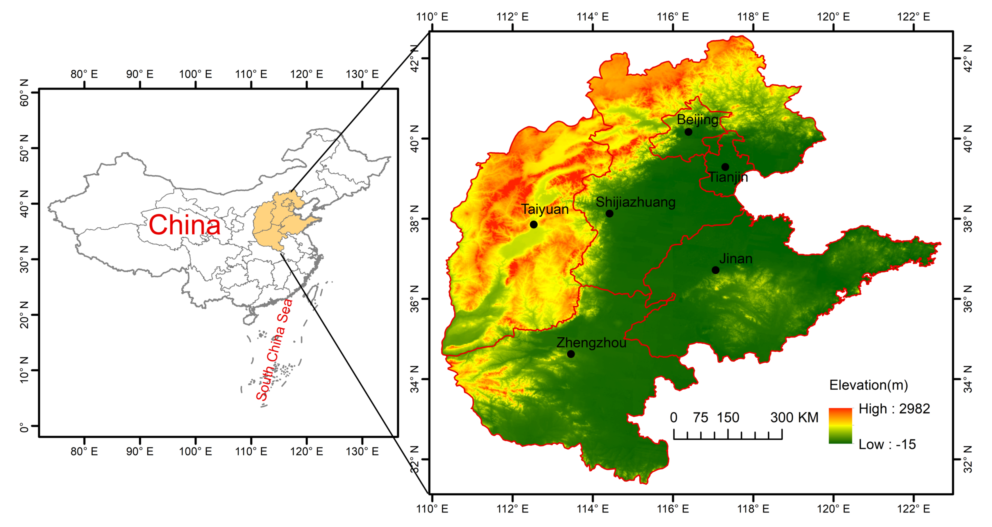
2. Study Area and Available Data

North China is embedded in an area with Yan Mountain in the north and Taihang Mountain in the west, which contributes to the accumulation of aerosols and leads to frequent pollution incidents [31]. Because North China, including the political and economic center of China, is one of the most polluted areas, Beijing, Tianjin, Shijiazhuang, Taiyuan, Zhengzhou and Jinan, being representative cities of North China, are selected as the sampling sites for atmosphere pollution analysis [31,32].

Figure 1 exhibits the distribution of sampling sites above. The research data include six pollutants monitored at a frequency of one hour [33]. The observation time of the research data spans from 1 January 2019 to 31 January 2019, including 744 observation samples, each of which is a vector composed of PM${}_{2.5}$, PM${}_{10}$, SO${}_2$, NO${}_2$, O${}_3$ and CO. Compared with daily or monthly data, hourly concentration data displays the stronger dependence in time dimension, that is, the prediction pollutant concentration is closely related to the neighbor samples. Therefore, it is very reasonable and meaningful for such data set to be selected to study the series neighbor structural information.

3. Methods

When machine learning algorithms are applied to time series prediction, it is inevitable to determine the functional relationship $y^{\prime }=f(X,Y)$ between the independent variable X, which is composed of the past time series, and the dependent variable Y (predicted values), where f represents the prediction model and $y^{\prime }$ is the prediction result. The normalized input variables of the prediction system are measured in equal interval observation, which can include both the historical values of the prediction target and the related influence factors. The task of the machine learning models is to build prediction model $y_{t+1}^{\prime }=f(X_t,\dots ,X_{t-n})$ in essence that uses the n-dimensional features with n lagged variable to interpret the input variables $X_i=\{x_{i,1},\dots ,x_{i,m}\}$. From the above analysis, we can find that in the modeling process of machine learning model, there is not enough attention to the structural characteristics, such as the sequence feature of time series data in time dimension and the noise interference of time series. We can think that the value of a certain time point in the time series is closely related to its adjacent data in its neighborhood, which is determined by the fitting function of the historical data in the neighborhood. Accordingly, for the sake of higher accurate prediction accuracy, it can be regarded as an effective means to mine the neighbor structural information.

3.1. Neighbor Structural Information Extraction Algorithm Based on Time Series Dynamic Decomposition

This paper proposes a method of extracting neighbor structural information based on dynamic decomposition, which can make full use of the unrevealed dynamics of time series. We first divide the time series into several parts to separate the dynamic modes that are helpful to the forecasting, then the optimal combination of the decomposed time series is carried out to extract the neighbor structural information. For any given series $r\left(t\right)$, it is well known that the prediction of $t_f$ time point mainly depends on the time series information before $t_f$. Further more, the value of $t_f$ is more sensitive to the time series data closer to it, that is, the data that are closer to $t_f$ in time dimension show stronger correlation. The dependence decays asymptotically to zero as the distance $\mathrm{dist}(t,t_f)\to \infty$. This characteristic will be reflected in the newly developed method.

We give an example to show the main idea of dynamic decomposition of the time series. For clear understanding, we consider the continuous time series. Let r be a sinusoidal signal with frequency $\omega$ and amplitude $\alpha$, i.e., $r\left(t\right)=\alpha sin\omega t$. Injecting r into two stable first order systems with zero initial state, we have

$${\dot{x}}_j\left(t\right)=-{\lambda }_j{x}_j\left(t\right)+r\left(t\right),x_j\left(0\right)=0,{\lambda }_j>0,j=1,2.$$

(1)

A simple computation shows that

$$x_j\left(t\right)=\frac{\alpha {\lambda }_j^2}{{\lambda }_j^2+{\omega }^2}\left(\frac{1}{{\lambda }_j}sin\omega t-\frac{\omega }{{\lambda }_j^2}cos\omega t+\frac{\omega }{{\lambda }_j^2}{e}^{-{\lambda }_{j}t}\right)$$

(2)

and thus

$$r\in \mathrm{span}\{x_1-{\epsilon }_1,x_2-{\epsilon }_2\},{\lambda }_1\ne {\lambda }_2,$$

(3)

where

$${\epsilon }_j\left(t\right)=\frac{\alpha {\lambda }_j^2}{{\lambda }_j^2+{\omega }^2}\frac{\omega }{{\lambda }_j^2}{e}^{-{\lambda }_{j}t}\to 0ast\to \infty ,j=1,2.$$

(4)

As a consequence of Formula (3), there exist two constants $k_1$ and $k_2$ such that

$$r\left(t\right)=k_1[x_1\left(t\right)-{\epsilon }_1\left(t\right)]+k_2[x_2\left(t\right)-{\epsilon }_2\left(t\right)],$$

(5)

which implies that, when t or ${\lambda }_j$ is large enough,

$$r\left(t\right)\approx \overline{r}\left(t\right)=k_1{x}_1\left(t\right)+k_2{x}_2\left(t\right).$$

(6)

The Formula (6) shows that the projection of r on the space $\mathrm{span}\{x_1-{\epsilon }_1,x_2-{\epsilon }_2\}$ can approximate r in some sense. Notice that

$$x_j\left(t\right)={\int }_0^t{e}^{-{\lambda }_j(t-s)}r\left(s\right)ds={\int }_0^t{e}^{-{\lambda }_{j}s}r(t-s)ds,$$

(7)

$x_j\left(t\right)$ is a weighted mean value of r with respect to the weight function $e^{-{\lambda }_{j}t}$. Since the weight function is exponentially stable, the time series decomposition mainly uses the neighbor structural information before t. Moreover, since system Equation (1) is stable, the high frequency noise added in r can be filtered. In other words, such an approximation is robust to the high frequency noise.

To sum up, there are four highlights for the dynamic series decomposition:

• Separate the dynamic modes hidden in the time series itself so that we can use the neighbor structural information sufficiently by optimized combination;
• We are able to choose the neighbor structural information by the tuning the parameter ${\lambda }_j$, $j=1,2$, that reflects the characteristic of the time series we mentioned above;
• Compared with machine learning models, the structural characteristics of time series data in time dimension are preserved;
• The white noise in the time series are filtered. So such a decomposition is robust to the white noise.

Now, we return to the general case. Suppose that $(A,B)$ is controllable with state space ${\mathbb{R}}^n$ and input space $\mathbb{R}$. Let $r\left(t\right)$ be a general time series. We divide the series r by the following system

$$\dot{x}\left(t\right)=Ax\left(t\right)+Br\left(t\right).$$

(8)

We solve Equation (8) to get

$$x\left(t\right)={(x_1\left(t\right),x_2\left(t\right),\cdots ,x_n\left(t\right))}^{\top }={\int }_0^t{e}^{A(t-s)}Br\left(s\right)ds,$$

(9)

which implies that the information of the injection $r\left(t\right)$ is decomposed into n parts and is contained in the components $x_j\left(t\right)$, $j=1,2,\cdots ,n$. Inspired by the aforementioned example, the projection of $\overline{r}$ on $\mathrm{span}\{x_1,x_2,\cdots ,x_n\}$ can approximate r effectively. Moreover, such an approximation is robust to the white noise in some sense because the high frequency noise can be filtered by the integral in Equation (9) provided A is Hurwitz.

The choice of A, B and the order n depends on the prior information of time series r. The tuning parameter $-\lambda \left(A\right)$ is the largest real part of eigenvalue of A, i.e., $\lambda \left(A\right)=max\left\{\mathrm{Re}s\right|s\in \sigma \left(A\right)\}$, where $\sigma \left(A\right)$ is the spectrum of the matrix A. Roughly speaking, the criterion of the order n is that guarantee n is lager than the modes that contained in r. The choice of $\lambda \left(A\right)$ is depends on the sampling frequency of the time series. The higher the frequency is, the larger the parameter $\lambda \left(A\right)$ is required.

3.2. The Hybrid Model Based on Neighbor Structural Information for PM${}_{2.5}$ Concentration Prediction

In order to utilize the neighbor structural information effectively, a hybrid model which combines the neighbor structural information with the traditional machine learning algorithm is proposed. The basic idea of the hybrid model is to integrate the neighbor structural information into the modeling data set in the form of input vector elements. Compared with the traditional modeling process, although the steps of neighbor structural information extraction will increase, the efficiency of the prediction system will not be reduced considering the simple implementation of the neighbor structural information extraction algorithm. It can be seen that the effectiveness of neighbor structural information is the key to improving the generalization ability of hybrid prediction system. The modeling flow of the hybrid system is illustrated by Figure 2, and the specific process based on neighbor structural information is shown via the following Algorithm 1.

Algorithm 1: PM${}_{2.5}$ concentration prediction hybrid model based on neighbor structural information

Require:  the data set ${\left\{(x_i,y_i)\right\}}_{i=1}^t$, where $x_i=(P{M}_{2.5_{i-1}},P{M}_{{10}_{i-1}},S{O}_{2_{i-1}},N{O}_{2_{i-1}},O_{3_{i-1}},C{O}_{i-1})$ is the input vector composed of influence factors at time i, and $y_i$ is the output formed by the concentration value of PM${}_{2.5}$ at the corresponding time. Ensure:  the prediction value $f\left(x_{t+1}^{{}^{\prime }}\right)$ of PM${}_{2.5}$ at time $t+1$. 1: Composing one-dimensional time series $r\left(t\right)=\{P{M}_{2.5_1},\dots ,P{M}_{2.5_t}\}$ with PM${}_{2.5}$ concentration values, and then obtaining the neighbor structural information $\{{\overline{r}}_1,\dots ,{\overline{r}}_t\}$ via the neighbor structural information extraction algorithm. 2: Forming the training data set ${\left\{(x_i^{{}^{\prime }},y_i)\right\}}_{i=1}^t$, where $x_i^{{}^{\prime }}=({\overline{r}}_{i-1},P{M}_{2.5_{i-1}},P{M}_{{10}_{i-1}},S{O}_{2_{i-1}},N{O}_{2_{i-1}},O_{3_{i-1}},C{O}_{i-1})$ entails the neighbor structural information ${\overline{r}}_{i-1}$ and $y_i$ is the PM${}_{2.5}$ concentration at time i. 3: According to the principle of the previous step, the input vector $x_{t+1}^{{}^{\prime }}=({\overline{r}}_t,P{M}_{2.5_t},P{M}_{{10}_t},S{O}_{2_t},N{O}_{2_t},O_{3_t},C{O}_t)$ of prediction model is constructed at time $t+1$. 4: Training the traditional machine learning algorithm on the previously constructed data set ${\left\{(x_i^{{}^{\prime }},y_i)\right\}}_{i=1}^t$, the optimal parameters are selected according to 10-fold cross validation. 5: Inputting the vector $x_{t+1}^{{}^{\prime }}$ at time $t+1$ into the prediction system of preceding training, the prediction result $f\left(x_{t+1}^{{}^{\prime }}\right)$ is obtained. The prediction results $f\left(x_{t+2}^{{}^{\prime }}\right),\dots ,f\left(x_{t+n}^{{}^{\prime }}\right)$ at $t+2,\dots ,t+n$ time can be obtained by iterating the above steps.

3.3. Performance Evaluation Index of Prediction Model

To prove the generalization ability of the hybrid prediction system with neighbor structural information, the measures describing system performance from different perspectives are applied in this study. They show how close the prediction values are to the observations. The measures used to evaluate performance here are: Mean Absolute Error (MAE), Mean Square Error (RMSE), Index of Agreement (IA), Direction Accuracy (DA), Mean Fractional Bias (MFB) and Mean Fractional Error (MFE).

$$\begin{array}{cc}\hfill MAE& =\frac{1}{n}\sum _{i=1}^n\mid y_i^{{}^{\prime }}-y_i\mid ,\hfill \end{array}$$

(10)

$$\begin{array}{cc}\hfill RMSE& =\sqrt[]{\frac{1}{n}\sum _{i=1}^n{(y_i^{{}^{\prime }}-y_i)}^2},\hfill \end{array}$$

(11)

$$\begin{array}{cc}\hfill IA& =1-\frac{{\sum }_{i=1}^n{(y_i^{{}^{\prime }}-y_i)}^2}{{\sum }_{i=1}^n\left(\right|y_i^{{}^{\prime }}-\overline{y}|+|y_i-\overline{y}{\left|\right)}^2},\hfill \end{array}$$

(12)

$$\begin{array}{cc}\hfill DA& =\frac{1}{n}\sum _{i=1}^n{w}_i,w_i=\left\{\begin{array}{c}1,if(y_{i+1}-y_i)(y_{i+1}^{{}^{\prime }}-y_i)>0,\hfill \\ 0,otherwise,\hfill \end{array}\right.\hfill \end{array}$$

(13)

$$MFB=\frac{2}{n}\sum _{i=1}^n\left(\frac{y_i^{{}^{\prime }}-y_i}{y_i^{{}^{\prime }}+y_i}\right)\times 100\%,$$

(14)

$$MFE=\frac{2}{n}\sum _{i=1}^n\left(\frac{|y_i^{{}^{\prime }}-y_i|}{y_i^{{}^{\prime }}+y_i}\right)\times 100\%,$$

(15)

in which, n is the sample size, $y_i$ means the observations, while $y_i^{{}^{\prime }}$ represents the prediction result obtained by the forecasting system.

MAE and RMSE display the error between the prediction values and the observed ones, which can also be understood as the closer to zero, the higher the forecasting accuracy of the algorithms. IA represents the correlation between the forecasts and the observations and DA indicates the prediction accuracy of the forecast results for the time series trend, of which larger values mean better prediction performance. The MFB and MFE values closing to zero represent better generalization ability of the prediction model.

4. Results and Discussion

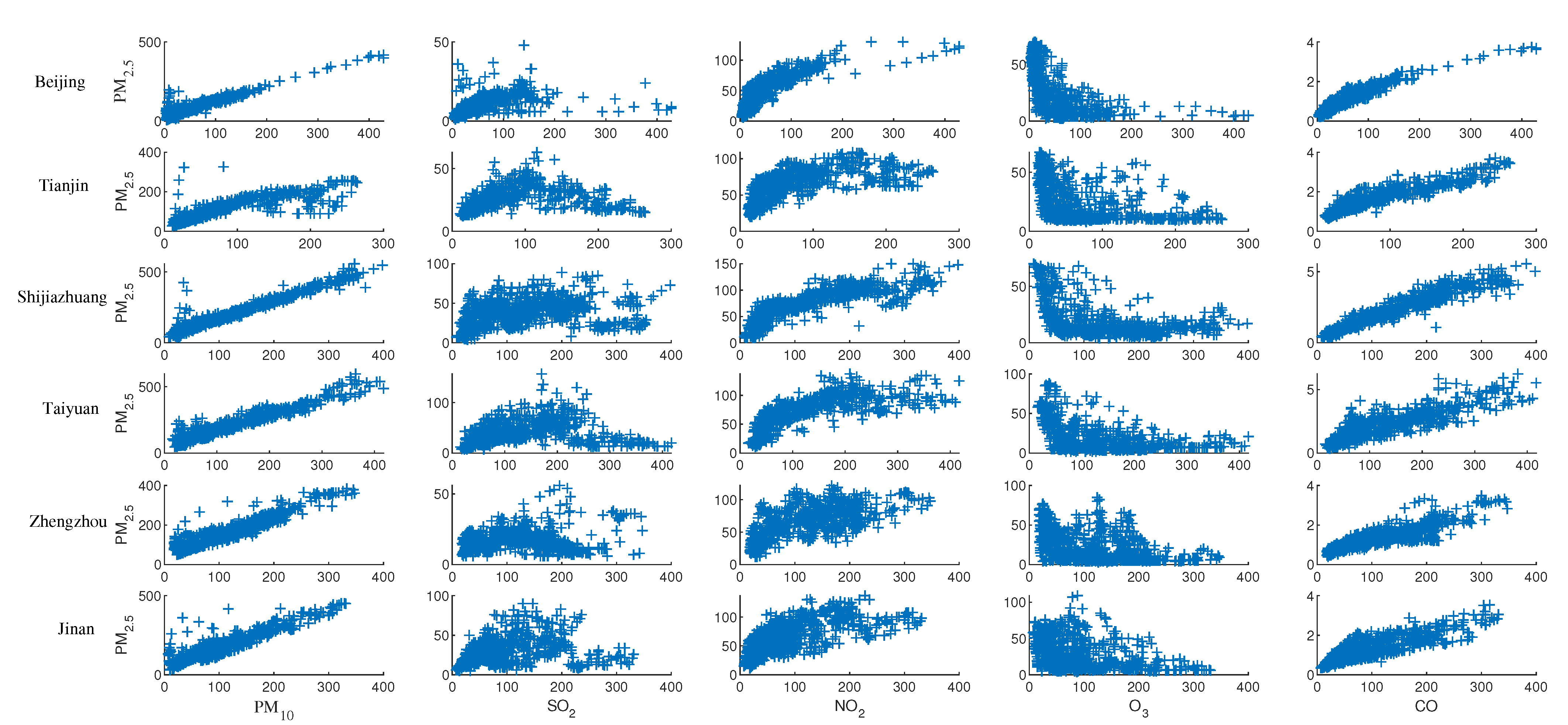
4.1. Data Statistics and Analysis

Table 1. Summary statistics for hourly air pollutants concentration (PM${}_{2.5}$, PM${}_{10}$, SO${}_2$, NO${}_2$, O${}_3$ and CO) from 1 January 2019 to 31 January 2019 in six monitoring sites.

Station	Air Pollutant	Mean	Median	Maximum	Minimum	Std.Dev.
Beijing	PM${}_{2.5}$ ($\mathsf{\mu }$g/m${}^3$)	50.20565	30.00000	428.0000	3.000000	57.88467
	PM${}_{10}$ ($\mathsf{\mu }$g/m${}^3$)	77.31048	65.00000	418.0000	5.000000	58.53817
	SO${}_2$ ($\mathsf{\mu }$g/m${}^3$)	8.561828	6.500000	48.00000	1.000000	6.011335
	NO${}_2$  ($\mathsf{\mu }$g/m${}^3$)	47.51747	50.00000	130.0000	6.000000	27.53585
	O${}_3$ ($\mathsf{\mu }$g/m${}^3$)	28.67070	23.50000	70.00000	2.000000	20.96675
	CO (mg/m${}^3$)	0.933587	0.750000	3.742000	0.209000	0.630729
Tianjin	PM${}_{2.5}$ ($\mathsf{\mu }$g/m${}^3$)	74.29704	53.00000	264.0000	11.00000	60.94219
	PM${}_{10}$ ($\mathsf{\mu }$g/m${}^3$)	102.0175	87.00000	326.0000	27.00000	54.85783
	SO${}_2$ ($\mathsf{\mu }$g/m${}^3$)	24.25269	23.00000	63.00000	12.00000	8.944761
	NO${}_2$ ($\mathsf{\mu }$g/m${}^3$)	62.98118	65.00000	109.0000	20.00000	21.53334
	O${}_3$ ($\mathsf{\mu }$g/m${}^3$)	25.21237	17.00000	67.00000	8.000000	16.87227
	CO (mg/m${}^3$)	1.531824	1.432000	3.706000	0.633000	0.645200
Shijiazhuang	PM${}_{2.5}$ ($\mathsf{\mu }$g/m${}^3$)	136.7097	121.0000	398.0000	8.000000	88.25823
	PM${}_{10}$ ($\mathsf{\mu }$g/m${}^3$)	220.4261	195.5000	558.0000	41.00000	111.2739
	SO${}_2$ ($\mathsf{\mu }$g/m${}^3$)	38.38978	39.00000	89.00000	4.000000	16.39194
	NO${}_2$ ($\mathsf{\mu }$g/m${}^3$)	76.67473	76.00000	150.0000	9.000000	27.84390
	O${}_3$ ($\mathsf{\mu }$g/m${}^3$)	19.95027	13.00000	70.00000	4.000000	15.83976
	CO (mg/m${}^3$)	2.239602	2.063000	5.563000	0.386000	1.163192
Taiyuan	PM${}_{2.5}$ ($\mathsf{\mu }$g/m${}^3$)	130.3347	109.0000	417.0000	16.00000	85.56525
	PM${}_{10}$ ($\mathsf{\mu }$g/m${}^3$)	211.0081	189.0000	597.0000	46.00000	104.2559
	SO${}_2$ ($\mathsf{\mu }$g/m${}^3$)	40.59812	37.00000	157.0000	7.000000	21.78152
	NO${}_2$ ($\mathsf{\mu }$g/m${}^3$)	72.69220	73.00000	137.0000	11.00000	25.47325
	O${}_3$ ($\mathsf{\mu }$g/m${}^3$)	18.66801	10.00000	88.00000	2.000000	18.33893
	CO (mg/m${}^3$)	2.145191	2.033000	6.225000	0.350000	1.103918
Zhengzhou	PM${}_{2.5}$ ($\mathsf{\mu }$g/m${}^3$)	121.5551	120.5000	347.0000	18.00000	74.17929
	PM${}_{10}$ ($\mathsf{\mu }$g/m${}^3$)	168.6075	164.0000	384.0000	50.00000	74.15855
	SO${}_2$ ($\mathsf{\mu }$g/m${}^3$)	16.93011	16.00000	56.00000	6.000000	7.428471
	NO${}_2$ ($\mathsf{\mu }$g/m${}^3$)	65.97043	67.00000	122.0000	12.00000	23.79673
	O${}_3$ ($\mathsf{\mu }$g/m${}^3$)	21.71371	14.00000	85.00000	3.000000	18.55841
	CO (mg/m${}^3$)	1.376922	1.282500	3.489000	0.383000	0.584595
Jinan	PM${}_{2.5}$ ($\mathsf{\mu }$g/m${}^3$)	94.49597	74.00000	331.0000	7.000000	69.41096
	PM${}_{10}$ ($\mathsf{\mu }$g/m${}^3$)	167.6237	143.0000	451.0000	30.00000	87.85827
	SO${}_2$ ($\mathsf{\mu }$g/m${}^3$)	28.67339	26.00000	90.00000	5.000000	15.59996
	NO${}_2$ ($\mathsf{\mu }$g/m${}^3$)	66.82796	67.00000	137.0000	11.00000	26.02158
	O${}_3$ ($\mathsf{\mu }$g/m${}^3$)	27.22312	19.00000	109.0000	4.000000	20.94018
	CO (mg/m${}^3$)	1.262667	1.125000	3.537000	0.338000	0.593352

lists the statistic results of monitoring concentration of six atmospheric pollutants used for atmospheric environment assessment, which are completed by Eviews software. The mean value of PM${}_{2.5}$ concentration in Shijiazhuang is the largest among those of the six research sites, reaching 136.7097 $\mathsf{\mu }$g/m${}^3$, which is far beyond the limit value 75 $\mathsf{\mu }$g/m${}^3$ of 24-hour average concentration issued by the National Ambient Air Quality Standard of China (GB 3095-2012) [34]. It is followed by Taiyuan with a PM${}_{2.5}$ concentration of 130.3347 $\mathsf{\mu }$g/m${}^3$. The main reason why PM${}_{2.5}$ concentration in these two cities exceeds the standard seriously is that there are more coal combustion for power and indoor heating supply in winter, accompanied by higher SO${}_4^{2-}$, and some coal-related ions such as NH${}_4^{+}$ and CL${}^{-}$ than other seasons [35,36,37]. In addition, PM${}_{2.5}$ concentration is further aggravated during the heating period. In particular, Beijing has the lowest mean PM${}_{2.5}$, but it shows the maximum monitoring value of 428.0000 $\mathsf{\mu }$g/m${}^3$ on 12 January 2019, which experienced a haze event. Generally, the high PM${}_{2.5}$ concentration of the six cities in North China prove that aerosol pollution in this area is an urgent problem. Further, it can be seen that the maximum of mean values of PM${}_{10}$, NO${}_2$ and CO appear in Shijiazhuang, the maximum value of SO${}_2$ is produced in Taiyuan, and the maximum value of O${}_3$ is represented in Beijing. According to the national standard, PM${}_{2.5}$ is the primary air pollutant currently monitored in most cases. Furthermore, Std.Dev. (Standard Deviation) demonstrates the degree to which the prediction values deviate from the mean value, and the maximum Std.Dev is obtained from the Shijiazhuang data set.

By analyzing the statistical results of monitored pollutants concentration, the distribution attributes at different stations are explored. PM${}_{2.5}$, owning the properties of mixed pollutants, has obvious correlation with other monitoring pollutants in theory. To explain more accurately the influence degree of PM${}_{2.5}$ by other air pollutants, Equation (16) is used to calculate the mutual information, which is described as follows.

$$\begin{array}{cc}\hfill I(X_{P{M}_{2.5}};Y_i)& =\sum _{x\in X_{P{M}_{2.5}}}\sum _{y_i\in Y_i}p(x,y_i)log\frac{p(x,y_i)}{p\left(x\right)p\left(y_i\right)},\hfill \end{array}$$

(16)

where X${}_{P{M}_{2.5}}$ and Y${}_i$ denote PM${}_{2.5}$ and a certain air pollutant, respectively.

Table 2. Results of mutual information between PM${}_{2.5}$ and other air pollutants (PM${}_{10}$, SO${}_2$, NO${}_2$, O${}_3$ and CO) during 1 January 2019 to 31 January 2019 study period in six monitoring sites. (The number in bold is the maximum mutual information value of the same monitoring site.)

Station	PM${}_{10}$	SO${}_2$	NO${}_2$	O${}_3$	CO
Beijing	4.4168	2.4362	3.8214	3.2117	1.0719
Tianjin	4.9867	3.0341	3.9941	2.9370	1.2865
Shijiazhuang	6.5212	4.2861	4.9755	3.6171	1.8261
Taiyuan	6.2537	4.4374	4.7564	3.5635	1.5286
Zhengzhou	5.7939	2.9521	4.5603	3.5413	1.1790
Jinan	5.7808	3.7637	4.5853	3.7543	0.9348

shows the results calculated according to Formula (16). The analysis results clearly show that PM${}_{2.5}$ of all sites possesses the largest mutual information with PM${}_{10}$, which verifies that the two variables have the strongest correlation. This is mainly due to the fact that PM${}_{2.5}$ and PM${}_{10}$ are both particulate pollutants, except for the difference in particle diameter. In terms of monitoring, PM${}_{10}$ concentration value covers the concentration value of PM${}_{2.5}$, so it is self-evident that they show a very strong coherence. Due to the same sources of pollution, PM${}_{2.5}$ is a large fraction (the majority) of PM${}_{10}$, ranging typically from 60% to 80% of PM${}_{10}$ [38]. Among the single pollutants, the mutual information values of NO${}_2$ in all data sets are greater than 3.8, which means that NO${}_2$ has a profound impact on PM${}_{2.5}$. Cities in North China are facing serious NO${}_2$ pollution, so the treatment of NO${}_2$ is beneficial for controlling PM${}_{2.5}$ concentration. Next, the air pollutant expressing strong correlation with PM${}_{2.5}$ is SO${}_2$ in Tianjin, Shijiazhuang, Taiyuan and Jinan, and O${}_3$ in Beijing and Zhengzhou. Although CO has the weakest influence on PM${}_{2.5}$ among all monitored pollutants, it is also an indispensable and important factor for PM${}_{2.5}$ forecasting. In addition, scatter plot (Figure 3) composed of features shows that PM${}_{2.5}$ represents a strong linear correlation with PM${}_{10}$ and CO; the relationship between PM${}_{2.5}$ and SO${}_2$, NO${}_2$ is more obvious linear relationship; while PM${}_{2.5}$ and O${}_3$ show a logarithmic correlation. It can be concluded that other pollutants have a great impact on PM${}_{2.5}$. The high correlation between air pollutants is due to the fact that they are affected by the same sources and experience the same meteorological influence (mainly transport and dispersal). It is very reasonable and scientific to select the above air pollutants as the input data of the prediction system.

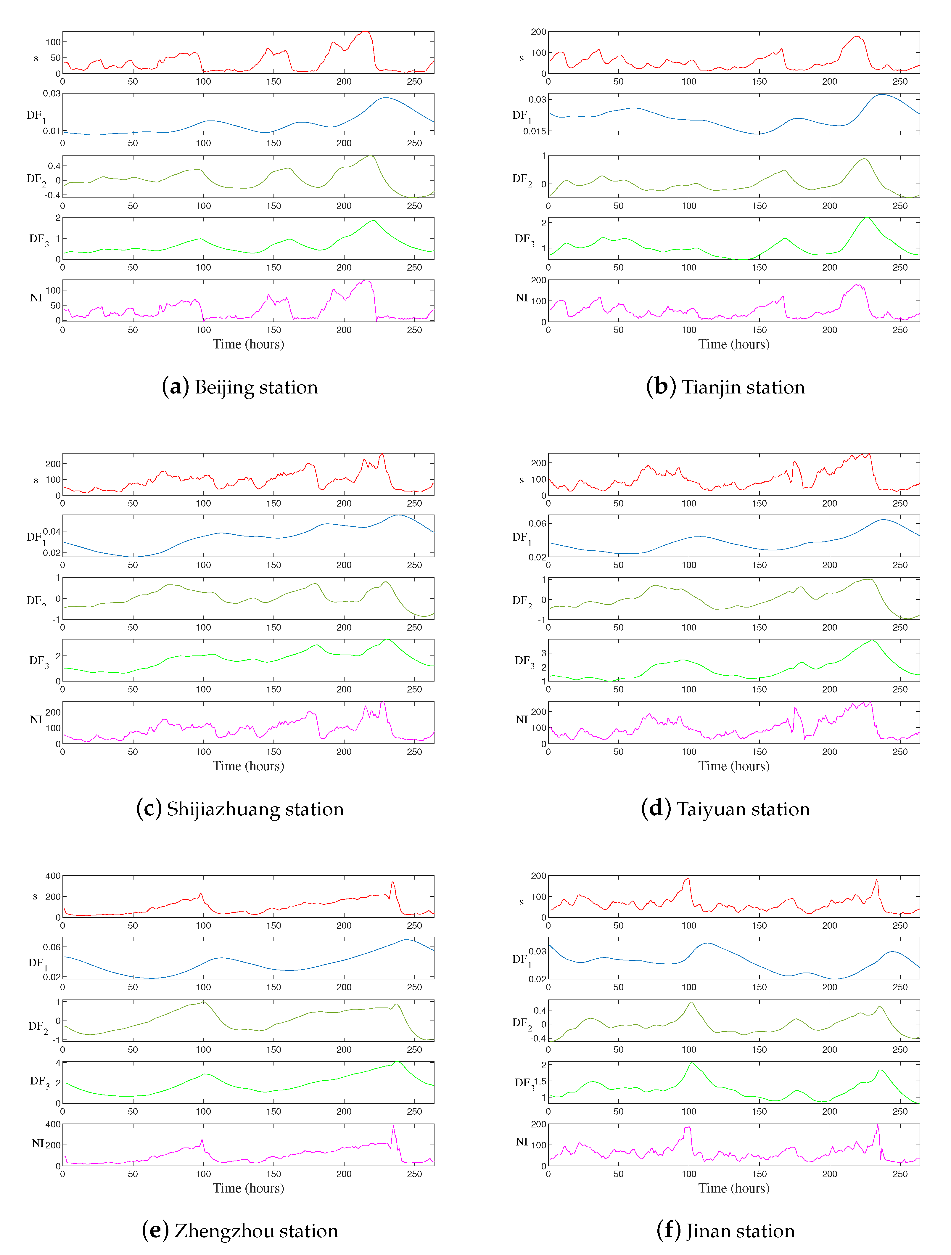
4.2. Neighbor Structural Information Extraction

For extracting the neighbor structural information and mining the structural characteristics of the original time series, this paper exploits neighbor structural information extraction algorithm based on dynamic decomposition that decomposes the original PM${}_{2.5}$ series into the dynamic modes, and then forms the neighbor structural information series by optimal combination. Figure 4 demonstrates that the original PM${}_{2.5}$ sequences are decomposed into three dynamic model subseries $D{F}_i,i=1,2,3$ with very similar frequencies and gradually increasing amplitudes, which are values in different feature directions in the dynamic modes space. NI is the series representing the neighbor structural information obtained by the optimal combination of the dynamic model subseries.

Table 3. Results of mutual information between PM${}_{2.5}$ and neighbor structural information during 21 January 2019 to 31 January 2019 test period in six monitoring sites.

Mutual Information	Beijing	Tianjin	Shijiazhuang	Taiyuan	Zhengzhou	Jinan
value	4.2167	4.9123	5.7812	5.6822	5.7278	4.9012

lists the mutual information values between the extracted neighbor structural information and PM${}_{2.5}$, which are all greater than 4.2, indicating that the neighbor structural information has a strong correlation with PM${}_{2.5}$. It can be concluded that the neighbor structural information effectively covers the structural information in the fields adjacent to the prediction points and has potential ability to improve the prediction accuracy.

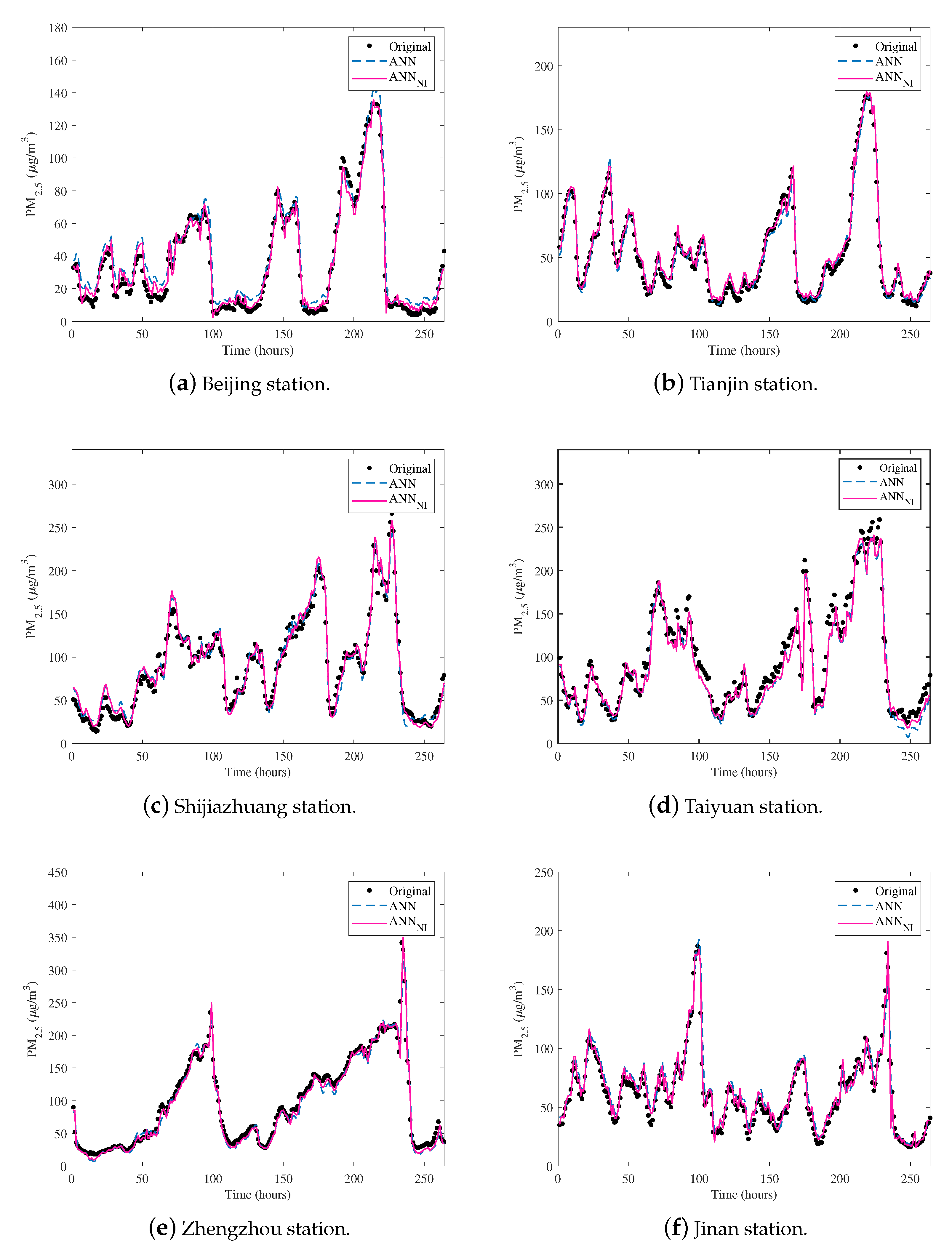
4.3. Results of the Hybrid Model Based on Neighbor Structural Information

In order to prove that the extracted neighbor structural information can be effectively integrated into the traditional machine learning algorithms, the representative single model ANN and SVM are selected as the basic models to construct the hybrid prediction system. The first 480 data in the experimental data set are allocated as training-validation data set, while the rest of data (264 samples) are used for testing.

4.3.1. Prediction Results Comparison between ANN and ANN${}_{NI}$

In the process of establishing ANN${}_{NI}$ model, the input layer comprises 7 nodes, the hidden layer contains 4 nodes, and the output layer is PM${}_{2.5}$ concentration. The logistic sigmoid function, as the well behaved function, is selected to realize the connection of hidden layer nodes. In addition, the parameters optimization in the models is implemented by cross validation method for the best prediction results.

The prediction performance assessment of ANN and ANN${}_{NI}$ is shown in

Table 4. Evaluation of prediction results of artificial neural network (ANN), ANN${}_{NI}$, support vector machine (SVM) and SVM${}_{NI}$ model for PM${}_{2.5}$ concentration for the test period (21–31 January 2019).

Data Set	Index	ANN	ANN${}_{\mathit{NI}}$	SVM	SVM${}_{\mathit{NI}}$
Beijing	MAE	6.5432	4.2307	4.3235	3.2980
	RMSE	8.2703	5.4690	6.4945	4.8231
	IA	0.9831	0.9923	0.9899	0.9944
	DA	0.6539	0.6996	0.6083	0.7034
	MFB	28.7589	13.0001	−2.2404	−1.4396
	MFE	31.4533	20.1745	19.9293	16.2861
Tianjin	MAE	5.3457	4.3846	4.7683	3.4534
	RMSE	7.2581	5.9939	7.5332	5.1871
	IA	0.9968	0.9979	0.9967	0.9984
	DA	0.5969	0.7262	0.6463	0.7756
	MFB	8.0473	1.5814	1.4136	1.2793
	MFE	11.5828	10.8061	10.3902	8.0389
Shijiazhuang	MAE	9.3995	8.5755	7.5206	7.3754
	RMSE	11.9466	10.9822	10.9781	10.5875
	IA	0.9967	0.9972	0.9972	0.9974
	DA	0.6045	0.6501	0.6958	0.6996
	MFB	3.1221	1.9686	−0.7779	−0.3174
	MFE	13.9759	12.1579	9.8720	9.7932
Taiyuan	MAE	12.6996	11.8033	9.2276	9.0214
	RMSE	17.0390	16.3416	14.0130	13.7118
	IA	0.9938	0.9943	0.9962	0.9963
	DA	0.5513	0.5551	0.6083	0.6387
	MFB	−14.0013	−8.5046	2.0742	1.3526
	MFE	18.6110	14.8266	11.0819	10.8000
Zhengzhou	MAE	8.5289	6.8320	5.9189	5.1456
	RMSE	13.6918	11.5107	12.7212	10.8639
	IA	0.9965	0.9975	0.9970	0.9978
	DA	0.5399	0.5893	0.6996	0.7604
	MFB	−8.5200	−7.7578	1.7476	0.9751
	MFE	13.2950	10.4419	7.0435	6.0181
Jinan	MAE	7.0559	5.4676	5.7105	4.8441
	RMSE	10.1595	8.4438	9.2179	8.2711
	IA	0.9949	0.9964	0.9957	0.9965
	DA	0.5741	0.6844	0.6121	0.7642
	MFB	6.9710	4.2608	1.0488	0.6914
	MFE	11.8254	9.5674	9.7819	8.2137

. The ANN${}_{NI}$ model integrates the neighbor structural information, and contains the implied structural characteristics of the PM${}_{2.5}$ series in the neighbor domain of the prediction points, so it can obtain better results under the indicators given in this paper. Table 4 lists the prediction errors of six data sets during the test period. MAEs of the hybrid ANN${}_{NI}$ models for different test sets are 4.2307, 4.3846, 8.5755, 11.8033, 6.8320 and 5.4676, respectively, which are significantly reduced compared with the 6.5432, 5.3457, 9.3995, 12.6996, 8.5289 and 7.0559 obtained by the basic model ANNs. Similarly, the same results can be obtained according to the values of RMSE. In addition, compared with ANNs, ANN${}_{NI}$ models have larger IA and DA, which means that ANN${}_{NI}$’s prediction values show stronger correlation with observed values and reflect more accurate trend judgment ability. Figure 5 shows the time series plots composed of test set prediction results and observations. We can observe from the graph that the predicted values of ANN and ANN${}_{NI}$ are very close to the observed values, indicating that the above prediction results are of high accuracy. However, at the extreme points and their adjacent points, ANN${}_{NI}$ models have more sensitive prediction ability, which benefits from their incorporation into the structural information of the neighbor domain. It is particularly noteworthy that the ANN${}_{NI}$ models need to determine the span of the neighbor domain in the process of extracting neighbor structural information, which is an application of the lags to a certain extent. By combining ANN with neighbor structural information, the prediction model not only obtains the ability to express the spatial characteristics of high-dimensional dynamic modes provided by neighbor structural information, but also helps to solve the problem that the lag order of ANN model is difficult to determine.

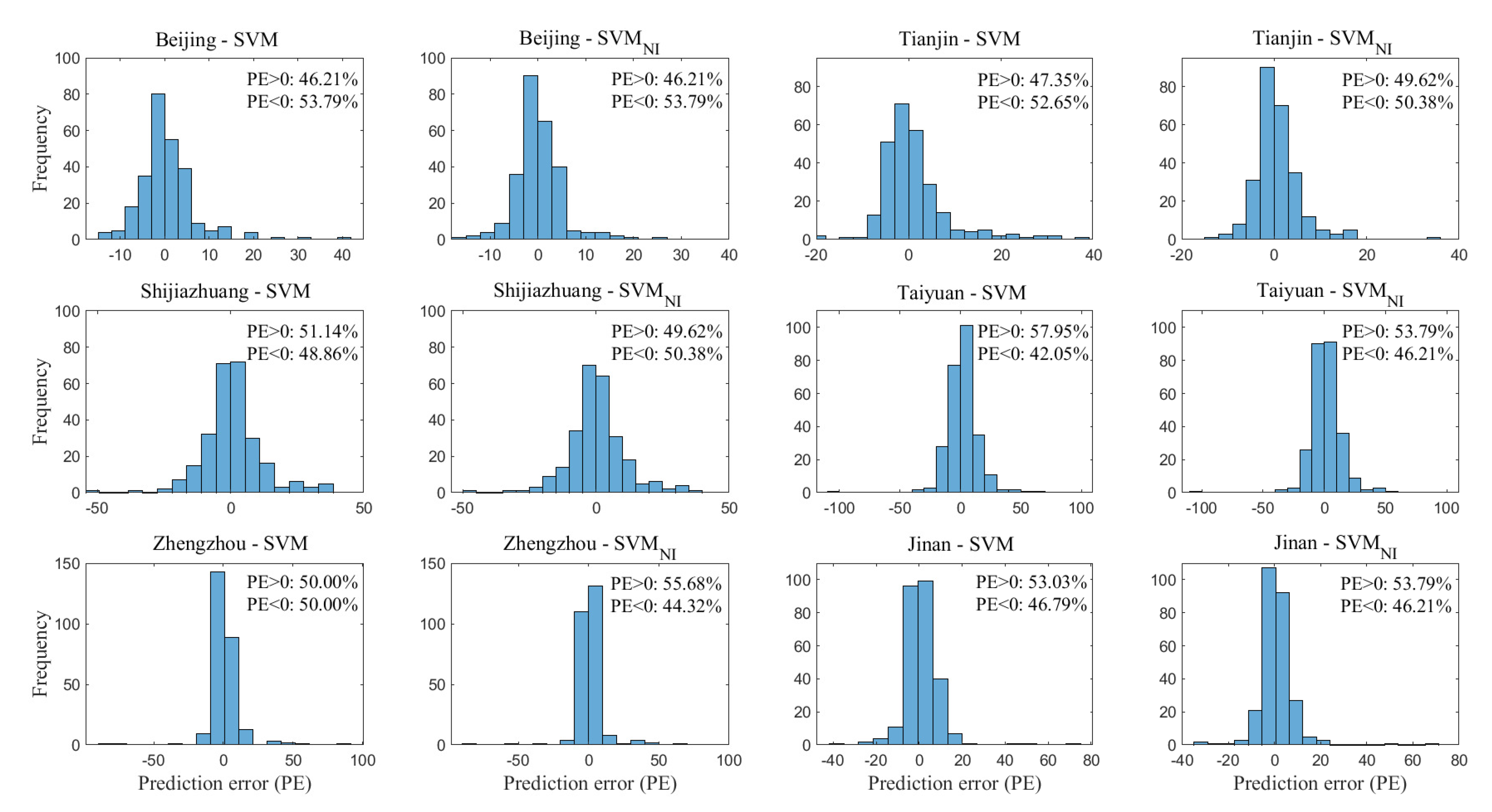
4.3.2. Prediction Results Comparison between SVM and SVM${}_{NI}$

SVM${}_{NI}$ is a hybrid system based on SVM, which contains neighbor structural information. SVM with structural risk minimization as the goal has a global optimal solution. However, when SVM is applied to time series prediction, the input vector is usually composed of historical data and influence factors, and then it is mapped to high-dimensional space by kernel function to obtain the optimal regression function. Therefore, the structural information of time series data cannot be reflected in the traditional SVM model. In the process of modeling, the gridsearch method is used to optimize the parameters. With optimal parameters, the prediction results of SVM and SVM${}_{NI}$ are given in Table 4 respectively. The MAE of SVM${}_{NI}$ on the Tianjin data set is 27.58% lower than that of SVM if performed best, which is followed by a 23.72% decline in Beijing. In terms of the Shijiazhuang data, SVM${}_{NI}$ demonstrates an ability to reduce MAE by 1.93%, which is not impressive enough though. For most data sets, SVM${}_{NI}$ can significantly improve the model accuracy, but it should be noted that the effect on individual data sets may not be obvious, on the premise of not reducing the generalization ability of the original model at least. Compared with SVM, the improvement of SVM${}_{NI}$’s IA index is not very effective, but the DA index has been greatly improved, indicating that SVM${}_{NI}$ can achieve more accurate trend prediction. Furthermore, Figure 6 shows the frequency distribution of prediction errors with different error ranges on each site test set, from which it can be observed that more prediction errors of SVM${}_{NI}$ model are around 0, compared with SVM model. In general, SVM${}_{NI}$’s prediction results are closer to the observed values, showing a higher prediction accuracy. Moreover, the applicability of the neighbor structural information to the SVM model further proves the robustness of the neighbor structural information extraction algorithm proposed in this paper.

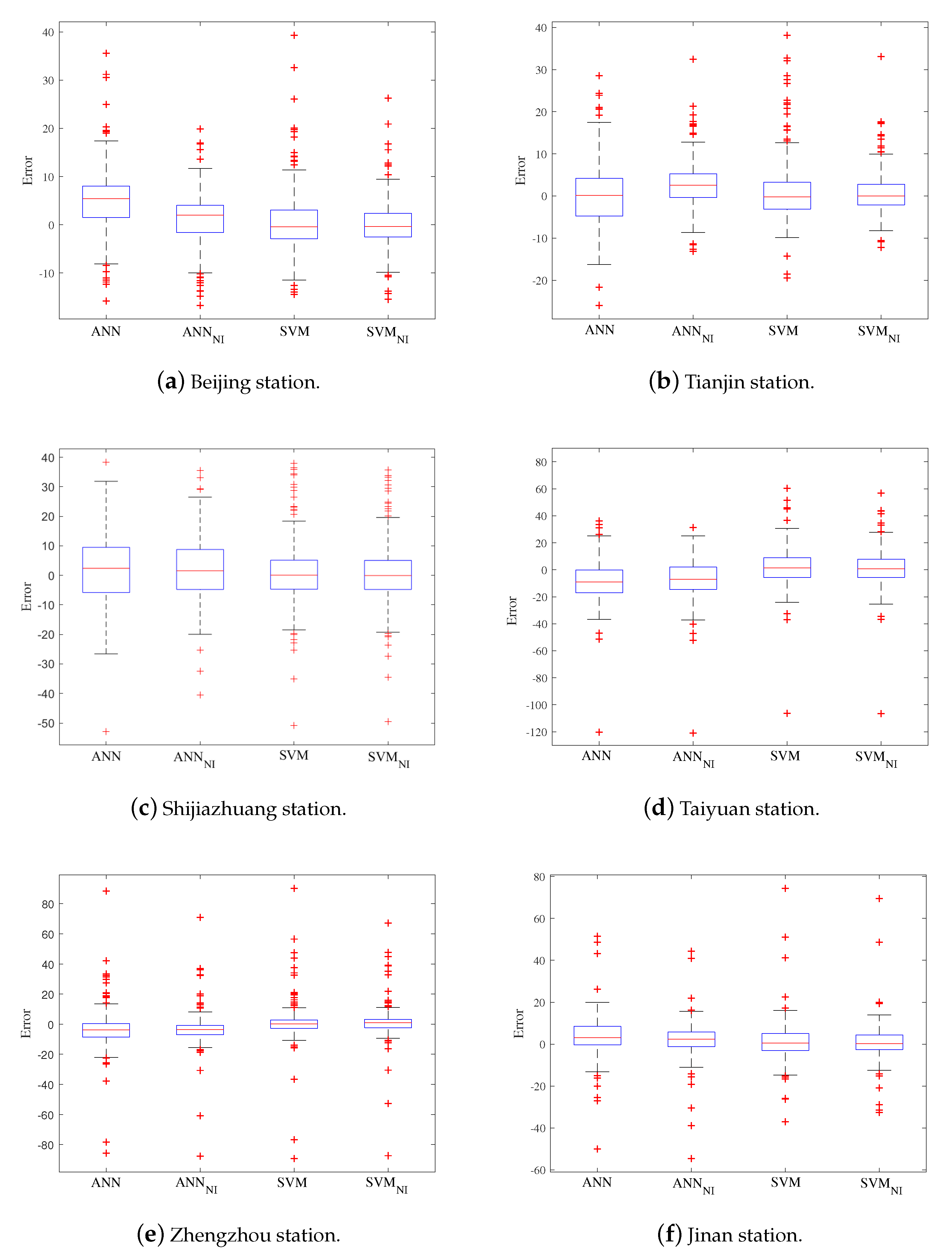
4.3.3. Prediction Results Comparison between ANN${}_{NI}$ and SVM${}_{NI}$

In this paper, the PM${}_{2.5}$ hybrid models ANN${}_{NI}$ and SVM${}_{NI}$ are based on the traditional ANN and SVM respectively, which can improve the generalization ability greatly. It is concluded that the proposed bybrid theory can improve the forecast system in many aspects, such as prediction accuracy, direction discrimination and correlation in accordance with the results of several performance criteria given in Table 4. Therefore, there is no doubt that the combination of neighbor structural information is helpful for mining the missing structural characteristic when machine learning algorithm is applied to time series forecast task. In addition, it is proved that the proposed neighbor structural information extraction algorithm based on dynamic decomposition is a significant technique to analyze the structural characteristics in time dimension. However, due to the difference of the basic models, the generalization ability of hybrid prediction system based on different machine learning algorithms is also different. As shown in Table 4, SVM${}_{NI}$’s prediction results are superior to the ANN${}_{NI}$ model in evaluation indexes. Due to the dynamics and timeliness of time series prediction, the capacity of training data set will not be large, so the SVM model for structural risk minimization is more appropriate for the case of small data set. In Figure 7, the prediction error range of the prediction models is shown by boxplots described by quartile values. According to the distribution characteristics of the prediction error results of different models, we notice that forecasting errors of hybrid systems are closer to 0. However, SVM${}_{NI}$ model is more accurate than ANN${}_{NI}$ model. In particular, it is worth paying attention to the fact that the outliers of SVM${}_{NI}$ are closer to 0, which means that SVM${}_{NI}$ can effectively correct outliers prediction. Figure 8 is the soccer plot composed of MFB and MFE indexes. The MFB and MFE values of the models fall into the continuous box, indicating that the prediction results are acceptable. Further more, they are in the dashed box, which means that the prediction model has good generalization ability. Figure 8 also clearly shows that the SVM${}_{NI}$ model’s statistical index results are closer to 0 than ANN${}_{NI}$’s. Especially for the MFB index of Beijing site, the result obtained by SVM${}_{NI}$ model strides into the area marking the accurate prediction results.

Table 5. Mean test of residual series of prediction models with or without neighbor structural information of six monitoring sites.

		ANN-SVM			ANN${}_{\mathit{NI}}$-SVM${}_{\mathit{NI}}$
Data Set	Mean	Std.Dev.	t-Statistic	Mean	Std.Dev.	t-Statistic
Beijing	2.219670 ***	3.807447	9.47236	0.932633 ***	2.347678	6.454671
	(0.0000)			(0.0000)
Tianjin	0.577466 **	4.044578	2.3198	0.931189 ***	2.158192	7.010516
	(0.0211)			(0.0000)
Shijiazhuang	1.878932 ***	6.838889	4.464033	1.200080 ***	5.994610	3.252753
	(0.0000)			(0.0013)
Taiyuan	3.472034 ***	9.939056	5.675979	2.781905 ***	9.295694	4.862532
	(0.0000)			(0.0000)
Zhengzhou	2.609981 ***	5.281503	8.029376	1.686462 ***	4.162686	6.582713
	(0.0000)			(0.0000)
Jinan	1.345375 ***	3.760126	5.813570	0.623489 ***	3.679429	2.753278
	(0.0000)			(0.0063)

Note: The number in the brackets is the p-Value, *** indicates the significance level of 1%, and ** indicates the significance level of 5%.

gives the mean test of model residuals with or without neighbor structural information. We notice that there is a significant difference between ANN and SVM, which may lead to the difference of prediction performance between ANN${}_{NI}$ and SVM${}_{NI}$.

5. Conclusions

Time series prediction of PM${}_{2.5}$ concentration is an essential and practical topic in the field of atmospheric research. Time series data has distinct characteristics in data structure, and its effective use is very helpful for the prediction system to obtain higher prediction accuracy. According to the modeling principle of machine learning algorithm, this paper proposes an algorithm of extracting neighbor structural information based on dynamic decomposition, and integrates it into machine learning model to construct a hybrid prediction model based on neighbor structural information. We use dynamic decomposition to decompose the original series into multiple dynamic modes to realize the structural information represented by the neighbor data, and then construct the neighbor structural information series through optimal combination. The simulation results of six groups of experimental data all show that the prediction model combined with neighbor structural information can obtain more accurate prediction results.

Therefore, the following conclusions can be drawn: (1) The method of time dynamic decomposition is suitable for the extraction of neighbor structural information representing the structural characteristics of time series. (2) The hybrid prediction model integrates the neighbor structural information to make up for the lack of structural characteristics of time series when machine learning models perform time series prediction. (3) The neighbor structural information extraction algorithm based on dynamic decomposition is generally applicable to traditional machine learning models. However, different basic machine learning algorithms lead to variant prediction ability of hybrid models. (4) The structural characteristics are inherent features of time series. Therefore, the algorithm proposed in this paper is also made available for other time series forecasting tasks in addition to PM${}_{2.5}$ concentration prediction.

References

1. Forouzanfar, M.H.; Afshin, A.; Alexander, L.T.; Anderson, H.R.; Bhutta, Z.A.; Biryukov, S.; Brauer, M.; Burnett, R.; Cercy, K.; Charlson, F.J.; et al. Global, regional, and national comparative risk assessment of 79 behavioural, environmental and occupational, and metabolic risks or clusters of risks, 1990–2015: A systematic analysis for the Global Burden of Disease Study 2015. Lancet 2016, 388, 1659–1724. [Google Scholar] [CrossRef] [Green Version]
2. Zheng, T.; Bergin, M.H.; Hu, S.; Miller, J.; Carlson, D.E. Estimating ground-level PM2.5 using micro-satellite images by a convolutional neural network and random forest approach. Atmos. Environ. 2020, 230, 117451. [Google Scholar] [CrossRef]
3. Niu, M.; Gan, K.; Sun, S.; Li, F. Application of decomposition-ensemble learning paradigm with phase space reconstruction for day-ahead PM2.5 concentration forecasting. J. Environ. Manag. 2017, 196, 110–118. [Google Scholar] [CrossRef]
4. Zhou, J.; Xing, Z.; Deng, J.; Du, K. Characterizing and sourcing ambient PM2.5 over key emission regions in China I: Water-soluble ions and carbonaceous fractions. Atmos. Environ. 2016, 135, 20–30. [Google Scholar] [CrossRef]
5. Zhang, L.; Yang, G.; Li, X. Mining sequential patterns of PM2.5 pollution between 338 cities in China. J. Environ. Manag. 2020, 262, 110341. [Google Scholar] [CrossRef]
6. Pui, D.Y.; Chen, S.C.; Zuo, Z. PM2.5 in China: Measurements, sources, visibility and health effects, and mitigation. Particuology 2014, 13, 1–26. [Google Scholar] [CrossRef]
7. Pak, U.; Ma, J.; Ryu, U.; Ryom, K.; Juhyok, U.; Pak, K.; Pak, C. Deep learning-based PM2.5 prediction considering the spatiotemporal correlations: A case study of Beijing, China. Sci. Total Environ. 2020, 699, 133561. [Google Scholar] [CrossRef]
8. Ding, L.; Zhu, D.; Peng, D.; Zhao, Y. Air pollution and asthma attacks in children: A case–crossover analysis in the city of Chongqing, China. Environ. Pollut. 2017, 220, 348–353. [Google Scholar] [CrossRef]
9. Lionetto, M.; Guascito, M.; Caricato, R.; Giordano, M.; Bartolomeo, A.; Romano, M.; Conte, M.; Dinoi, A.; Contini, D. Correlation of Oxidative Potential with Ecotoxicological and Cytotoxicological Potential of PM10 at an Urban Background Site in Italy. Atmosphere 2019, 10, 733. [Google Scholar] [CrossRef] [Green Version]
10. Shen, R.; Liu, Z.; Chen, X.; Wang, Y.; Wang, L.; Liu, Y.; Li, X. Atmospheric levels, variations, sources and health risk of PM2.5-bound polycyclic aromatic hydrocarbons during winter over the North China Plain. Sci. Total Environ. 2019, 655, 581–590. [Google Scholar] [CrossRef]
11. Liu, Z.; Hu, B.; Zhang, J.; Yu, Y.; Wang, Y. Characteristics of aerosol size distributions and chemical compositions during wintertime pollution episodes in Beijing. Atmos. Res. 2016, 168, 1–12. [Google Scholar] [CrossRef]
12. Qi, Y.; Li, Q.; Karimian, H.; Liu, D. A hybrid model for spatiotemporal forecasting of PM2.5 based on graph convolutional neural network and long short-term memory. Sci. Total Environ. 2019, 664, 1–10. [Google Scholar] [CrossRef] [PubMed]
13. Bray, C.D.; Battye, W.; Aneja, V.P.; Tong, D.; Lee, P.; Tang, Y.; Nowak, J.B. Evaluating ammonia (NH3) predictions in the NOAA National Air Quality Forecast Capability (NAQFC) using in-situ aircraft and satellite measurements from the CalNex2010 campaign. Atmos. Environ. 2017, 163, 65–76. [Google Scholar] [CrossRef]
14. Woody, M.; Wong, H.W.; West, J.; Arunachalam, S. Multiscale predictions of aviation-attributable PM2.5 for U.S. airports modeled using CMAQ with plume-in-grid and an aircraft-specific 1-D emission model. Atmos. Environ. 2016, 147, 384–394. [Google Scholar] [CrossRef]
15. Zhou, Y.; Chang, F.J.; Chang, L.C.; Kao, I.F.; Wang, Y.S.; Kang, C.C. Multi-output support vector machine for regional multi-step-ahead PM2.5 forecasting. Sci. Total Environ. 2019, 651, 230–240. [Google Scholar] [CrossRef]
16. Lv, B.; Cobourn, W.G.; Bai, Y. Development of nonlinear empirical models to forecast daily PM2.5 and ozone levels in three large Chinese cities. Atmos. Environ. 2016, 147, 209–223. [Google Scholar] [CrossRef]
17. Cobourn, W.G. An enhanced PM2.5 air quality forecast model based on nonlinear regression and back-trajectory concentrations. Atmos. Environ. 2010, 44, 3015–3023. [Google Scholar] [CrossRef]
18. Suleiman, A.; Tight, M.; Quinn, A. Applying machine learning methods in managing urban concentrations of traffic-related particulate matter (PM10 and PM2.5). Atmos. Pollut. Res. 2019, 10, 134–144. [Google Scholar] [CrossRef]
19. Catalano, M.; Galatioto, F.; Bell, M.; Namdeo, A.; Bergantino, A.S. Improving the prediction of air pollution peak episodes generated by urban transport networks. Environ. Sci. Policy 2016, 60, 69–83. [Google Scholar] [CrossRef] [Green Version]
20. Ragosta, M.; D’Emilio, M.; Giorgio, G. Input strategy analysis for an air quality data modelling procedure at a local scale based on neural network. Environ. Monit. Assess. 2015, 187, 4556. [Google Scholar] [CrossRef]
21. Zhou, Q.; Jiang, H.; Wang, J.; Zhou, J. A hybrid model for PM2.5 forecasting based on ensemble empirical mode decomposition and a general regression neural network. Sci. Total Environ. 2014, 496, 264–274. [Google Scholar] [CrossRef] [PubMed]
22. MA, J.; Ding, Y.; Cheng, J.C.; Jiang, F.; Wan, Z. A Temporal-Spatial Interpolation and Extrapolation Method Based on Geographic Long Short-Term Memory Neural Network for PM2.5. J. Clean. Prod. 2019, 237, 117729. [Google Scholar] [CrossRef]
23. Zhou, Y.; Chang, F.J.; Chen, H.; Li, H. Exploring Copula-based Bayesian Model Averaging with multiple ANNs for PM2.5 ensemble forecasts. J. Clean. Prod. 2020, 263, 121528. [Google Scholar] [CrossRef]
24. Yang, W.; Deng, M.; Xu, F.; Wang, H. Prediction of hourly PM2.5 using a space-time support vector regression model. Atmos. Environ. 2018, 181, 12–19. [Google Scholar] [CrossRef]
25. Biancofiore, F.; Busilacchio, M.; Verdecchia, M.; Tomassetti, B.; Aruffo, E.; Bianco, S.; Tommaso, S.D.; Colangeli, C.; Rosatelli, G.; Carlo, P.D. Recursive neural network model for analysis and forecast of PM10 and PM2.5. Atmos. Pollut. Res. 2017, 8, 652–659. [Google Scholar] [CrossRef]
26. Neto, P.S.G.D.M.; Marinho, M.H.N.; Siqueira, H.; Tadano, Y.D.S.; Machado, V.; Alves, T.A.; Oliveira, J.F.L.D.; Madeiro, F. A Methodology to Increase the Accuracy of Particulate Matter Predictors Based on Time Decomposition. Sustainability 2020, 12, 7310. [Google Scholar] [CrossRef]
27. Crone, S.F.; Kourentzes, N. Feature selection for time series prediction—A combined filter and wrapper approach for neural networks. Neurocomputing 2010, 73, 1923–1936. [Google Scholar] [CrossRef] [Green Version]
28. Mouatadid, S.; Raj, N.; Deo, R.C.; Adamowski, J.F. Input selection and data-driven model performance optimization to predict the Standardized Precipitation and Evaporation Index in a drought-prone region. Atmos. Res. 2018, 212, 130–149. [Google Scholar] [CrossRef]
29. Zhang, C.; Zhou, J.; Li, C.; Fu, W.; Peng, T. A compound structure of ELM based on feature selection and parameter optimization using hybrid backtracking search algorithm for wind speed forecasting. Energy Convers. Manag. 2017, 143, 360–376. [Google Scholar] [CrossRef]
30. Shukur, O.B.; Lee, M.H. Daily wind speed forecasting through hybrid KF-ANN model based on ARIMA. Renew. Energy 2015, 76, 637–647. [Google Scholar] [CrossRef]
31. Song, Z.; Fu, D.; Zhang, X.; Han, X.; Song, J.; Zhang, J.; Wang, J.; Xia, X. MODIS AOD sampling rate and its effect on PM2.5 estimation in North China. Atmos. Environ. 2019, 209, 14–22. [Google Scholar] [CrossRef]
32. Li, M.; Wang, L.; Liu, J.; Gao, W.; Song, T.; Sun, Y.; Li, L.; Li, X.; Wang, Y.; Liu, L.; et al. Exploring the regional pollution characteristics and meteorological formation mechanism of PM2.5 in North China during 2013–2017. Environ. Int. 2020, 134, 105283. [Google Scholar] [CrossRef] [PubMed]
33. Lv, Z.; Wei, W.; Cheng, S.; Han, X.; Wang, X. Meteorological characteristics within boundary layer and its influence on PM2.5 pollution in six cities of North China based on WRF-Chem. Atmos. Environ. 2020, 228, 117417. [Google Scholar] [CrossRef]
34. Lai, S.; Zhao, Y.; Ding, A.; Zhang, Y.; Song, T.; Zheng, J.; Ho, K.F.; Lee, S.C.; Zhong, L. Characterization of PM2.5 and the major chemical components during a 1-year campaign in rural Guangzhou, Southern China. Atmos. Res. 2016, 167, 208–215. [Google Scholar] [CrossRef]
35. He, Q.; Yan, Y.; Guo, L.; Zhang, Y.; Zhang, G.; Wang, X. Characterization and source analysis of water-soluble inorganic ionic species in PM2.5 in Taiyuan city, China. Atmos. Res. 2017, 184, 48–55. [Google Scholar] [CrossRef]
36. Meng, Z.; Jiang, X.; Yan, P.; Lin, W.; Zhang, H.; Wang, Y. Characteristics and sources of PM2.5 and carbonaceous species during winter in Taiyuan, China. Atmos. Environ. 2007, 41, 6901–6908. [Google Scholar] [CrossRef]
37. Zhang, H.; Cheng, S.; Li, J.; Yao, S.; Wang, X. Investigating the aerosol mass and chemical components characteristics and feedback effects on the meteorological factors in the Beijing-Tianjin-Hebei region, China. Environ. Pollut. 2019, 244, 495–502. [Google Scholar] [CrossRef]
38. Cesari, D.; De Benedetto, G.; Bonasoni, P.; Busetto, M.; Dinoi, A.; Merico, E.; Chirizzi, D.; Cristofanelli, P.; Donateo, A.; Grasso, F.; et al. Seasonal variability of PM2.5 and PM10 composition and sources in an urban background site in Southern Italy. Sci. Total Environ. 2018, 612, 202–213. [Google Scholar] [CrossRef]
Figure 1. DEM map of the studied area with data acquisition sites (solid black circle).
Sustainability 13 00447 g001
Figure 2. The hybrid model based on neighbor structural information construction framework.
Sustainability 13 00447 g002
Figure 3. Scatter plots of relationship between PM 2.5 and impact factors (PM 10 , SO 2 , NO 2 , O 3 and CO) during 1 January 2019 to 31 January 2019 study period in six monitoring sites.
Sustainability 13 00447 g003
Figure 4. Dynamic decomposition results of six monitoring sites for the test period (21–31 January 2019). D F i , i = 1 , 2 , 3 is dynamic model subseries and NI is the neighbor structural information series.
Sustainability 13 00447 g004
Figure 5. Time series plots of forecasts and the original values of the PM 2.5 concentration, calculated by the ANN model and the ANN N I model for the test period (21–31 January 2019).
Sustainability 13 00447 g005
Figure 6. Histograms of the frequency distribution of prediction error (PE) for the PM 2.5 concentration, calculated by the SVM model and the SVM N I model for the test period (21–31 January 2019).
Sustainability 13 00447 g006
Figure 7. Boxplot of the prediction error of PM 2.5 concentration using ANN, ANN N I , SVM and SVM N I for the test period (21–31 January 2019).
Sustainability 13 00447 g007
Figure 8. Soccer plot composed of Mean Fractional Bias (MFB) and Mean Fractional Error (MFE) indexes of ANN N I and SVM N I prediction results. The shapes represent the prediction results of different sites from 21–31 January 2019.
Sustainability 13 00447 g008