Evaluating the Impact of Floods on Housing Price Using a Spatial Matching Difference-In-Differences (SM-DID) Approach


1
École supérieure d’aménagement du territoire et de développement régional (ESAD), Université Laval, Québec, QC G1V 0A6, Canada
2
INRS-UCS, Montréal, QC H2X 1E3, Canada
3
UQAR, Rimouski, QC G5L 3A1, Canada
*
Author to whom correspondence should be addressed.
Sustainability 2021, 13(2), 804; https://0-doi-org.brum.beds.ac.uk/10.3390/su13020804
Submission received: 22 December 2020
/
Revised: 11 January 2021
/
Accepted: 13 January 2021
/
Published: 15 January 2021
(This article belongs to the Section Hazards and Sustainability)
Abstract
:Many applications have relied on the hedonic pricing model (HPM) to measure the willingness-to-pay (WTP) for urban externalities and natural disasters. The classic HPM regresses housing price on a complete list of attributes/characteristics that include spatial or environmental amenities (or disamenities), such as floods, to retrieve the gradients of the market (marginal) WTP for such externalities. The aim of this paper is to propose an innovative methodological framework that extends the causal relations based on a spatial matching difference-in-differences (SM-DID) estimator, and which attempts to calculate the difference between sale price for similar goods within “treated” and “control” groups. To demonstrate the potential of the proposed spatial matching method, the researchers present an empirical investigation based on the case of a flood event recorded in the city of Laval (Québec, Canada) in 1998, using information on transactions occurring between 1995 and 2001. The research results show that the impact of flooding brings a negative premium on the housing price of about 20,000$ Canadian (CAN).
1. Introduction
City life involves a complex array of attractive (i.e., positive) and unattractive (i.e., negative) features, which urban economists call externalities and that are described as being unpriced and non-market amenities because there exists no official market for such effects. Externalities can be related to urban or non-urban or environmental components. Examples of urban externalities include noise, traffic congestion, pollution and crime. Examples of non-urban externalities include those related to natural disasters such as floods, fire, earthquakes and erosion. Yet, measuring the economic impact of such externalities still poses a challenge to scholars worldwide ([1]).
Since its development by Rosen in 1974 ([2]), many applications have relied on hedonics, which is an approach based on revealed preferences, to measure the willingness-to-pay (WTP) of the market to avoid negative externalities or to benefit from positive externalities. Hedonic pricing models (HPM) have been widely applied to the real-estate market to measure and estimate the value of urban as well as non-urban/environmental amenities and externalities. Many of these externalities are usually qualified as “exogenous shocks”, at least from an individual economic agent’s perspective. Although such hedonic applications are considered fairly straightforward, many challenges still remain to adequately measure or rather estimate the effect of urban externalities, or environmental amenities, on values of real-estate property.
One of these challenges is to make sure that the omission variable bias is adequately controlled for in the regression analysis (i.e., the exhaustive list of a complex good ’s characteristics is observed and included in the statistical model). The presence of latent information can introduce bias in the estimated WTP if it happens to be correlated with the externalities of interest. This could consequently invalidate the conclusions drawn from the statistical analysis. Another challenge to applying HPMs to measure externalities is to make sure that the WTP adequately represents a causal relation, i.e., that the externality is causing the price, and not the opposite. Major roads and their impact on housing price is a good example of reverse causality: major roads cause negative externalities, which influence housing price. However, roads are also built and located within axes where house prices are lower. Thus, isolating the causal relation (dealing with endogeneity) is also a challenge that researchers face while using HPM and that could lead to an invalidation of results.
An interesting approach to correctly isolate the impact of environmental amenities on the housing price would be to use information on changes (or shock) that occur over time. In such a case, the difference-in-differences (DID) estimator ([3,4,5]), including its extension to the spatial ([6,7]) and the spatiotemporal case ([8]), presents an adapted methodological framework that can be used to isolate causal relations from a statistical framework. The DID estimator is one of many possible approaches to investigate causal relations ([9]). However, the precision of the estimation obtained using the DID approach also depends on some major assumptions ([10]).
The aim of this paper is to propose a new methodological framework that uses a spatial matching estimator that is based on the DID approach. The resulting methodological proposition, a spatial matching difference-in-differences (SM-DID) estimator, is advantageous in many aspects. Firstly, it explicitly exposes a clear link between the matching approach and that adopted in professional practice which is usually based on the comparable sales approach (CSA). This makes the proposed approach quite intuitive ([11]). Secondly, the proposed approach greatly simplifies the statistical procedure used for estimating the effect of a local change that occurs in a quasi-natural (or natural) experiment and adequately deals with the potential problems related to the existence of a sub-market. Thirdly, the presented approach can deal with a relatively small number of transactions (observations) which is advantageous and a promising avenue for further investigation, especially when studying the impact of externalities in non-urban and rural areas. To demonstrate the potential of the proposed spatial matching DID estimator (SM-DID), an empirical investigation that is based on the case of a 1998 flood event recorded in the city of Laval (Québec, Canada) and on information on house sale transactions occurring in a given neighborhood between the years 1995 and 2001 is presented. The results suggest that the methodology is promising and estimate the impact of flooding on single-family houses to be a negative premium of about 20,000$ CAN.
The paper is divided into eight sections. The Section 2 is a brief introduction on flood literature. The Section 3 presents a brief overview of the use of the hedonic pricing model HPM and its descendent, the DID estimator, for measuring the effect of urban externalities, showing its clear link with the comparable sales approach which is a popular method among real estate professionals. This section formally demonstrates how the proposed ‘matching’ estimator/methodological framework can be used to isolate the impact of a given extrinsic amenity. The Section 4 is a thorough explanation of how to identify the “comparable(s)” in “treatment” and “control” groups. The Section 5 presents the data used to implement the methodological framework on the case of flood to investigate its expected effect on the price of single-family housing. The Section 6 presents the results followed by a formal discussion of their implications.
2. Materials and Methods
The flood literature has been quite dominant in the past few years. Floods have been constantly and repeatedly hitting, especially in recent years, as a result of climate change. Floods are the costliest natural disasters in Canada ([12]) with an average loss of 1–2 billion dollars per year ([13]). As a result, it is expected that floods might have an influence on real estate prices.
However, the investigation of the effect of floods (as an environmental disamenity) on real estate property prices is far from being a straightforward pursuit. Franco and Macdonald ([14]) state that there has been a volume of work on floods with a number of studies concentrating on the effect of flood risk, while others on the occurrence of floods or flash floods and their impact on the real estate market. Existing studies on the effect of natural hazards on residential prices show that the market responds to such an environmental disamenity by a decrease in the property price that is located in flood zones ([15,16,17,18,19]).
The vast heterogeneity of results suggests a relationship between floods and housing price that has its own specificity. Floods are phenomena of nature that happen when lakes, streams and rivers overflow their natural banks. As a natural disaster, a flood is defined by the damage it causes to people or property ([20,21]). However, flood areas are considered attractive and a pulling force for human settlement because of human convenience for plenty of various reasons that include the attractive view, transportation, water supply and the rich agricultural soil ([22]). In Canada, as in other places of the world, flood maps are created to demark areas prone to being flooded in the case of water mounting to a certain elevation. As such, flood maps demarking floodplains provide stakeholders with essential data to make the decisions needed in case of the management of flood risk or in issues regarding urban planning or asset management ([23] Squareoneinsurance.com, 2020). In general, floodplain designation is an identification of areas that are to be flooded with a sort of annual frequency, for example, once in a span of 20 or 100 years. As such, a floodplain depicts areas that are subjected to “a reasonable risk of flooding” (i.e., a floodplain is a demarcation where there is a probability that a flood event occurs in a certain land unit) ([24]).
Surveying the literature, Beltrán et al. ([25]) state that the price discount ranges between −75.5% and +61% of a price premium. This dramatic difference could be explained by numerous reasons. One plausible reason might be that many studies fail to distinguish between properties that are located inside flood zones and those that were ‘actually’ flooded, which results in a huge problem in the interpretation of results ([26]). Another reason might be that floods are localized events. A global and more convincing reason might be that the methodologies currently used in the investigation of the price of environmental externalities are still in need of correction. So far, most studies compare the sale price for properties located inside a flooding zone, which is usually defined as being located inside versus outside a 100- or a 500-year flood zone ([27,28,29,30,31,32]).
The methodology presented in this research aims to fill the gap in the literature by providing an innovative framework that incorporates the recent literature while taking into consideration the spatiotemporal reality of the price determination process ([8]), where counterfactuals are identified by calculating the smallest distances, over space and characteristics.
2.1. Measuring Urban Externalities: The Hedonic Pricing Model (HPM)
The hedonic pricing theory was formally defined by Rosen ([2]). However, even long before his pioneering work, many empirical applications adopted a similar framework, which simply consists of expressing, through a statistical model, the sale price of a complex good i sold at time t. yit is a function of the individual (intrinsic and extrinsic) amenities that form a bundle that describes a real estate good (Equation (1)).
y = αι + Xβ + ε
The sale prices are stacked in a vector y of dimension (NT × 1), that is usually expressed in a logarithmic transformation; the list of independent variables is stacked in a matrix X of dimension (NT × K), ι is a vector of one, and ε is a vector of errors; both are of dimension (NT × 1), where NT is the total sample size (NT = ∑tNt). The vector of parameters β, of dimension (K × 1), captures the implicit price of each amenity, including the intrinsic as well as the extrinsic amenities, while α is a scalar, constant term parameter. As such, the estimation of the price equation is considered to be quite straightforward and allows one to obtain the implicit price related to extrinsic amenities ([33]).
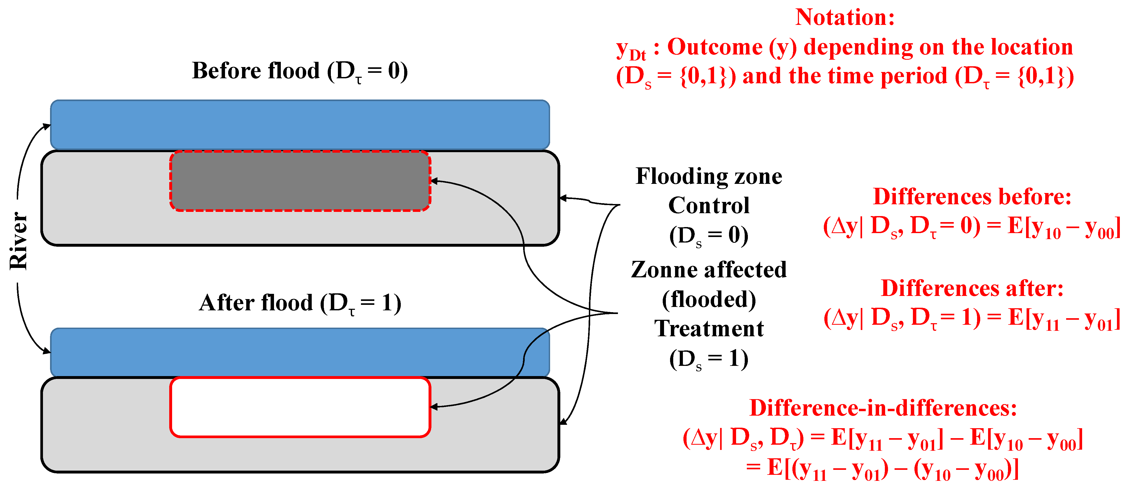
The temporal dimension of the transaction information can actually be exploited to adequately control for endogeneity and causality issues. In such a case, a difference-in-differences (DID) estimator ([4,5]) is used to isolate the impact of a change in a given amenity within two periods (before and after an exogenous change–Dτ = {0,1}) in a specific location (within treatment and control areas–Ds = {0,1}). The DID estimator adequately makes it possible to isolate the contribution of one specific amenity after a given, assumed exogenous change or shock occurring in the urban space or landscape. By introducing these two additional variables, one obtains the HPM-DID specification (Equation (2)).
where δs is a matrix of coefficients isolating the impact of being inside the spatial delimitation where the change occurs, δτ is a matrix identifying the impact related to any temporal modification in the price determination process, and γ is a matrix of coefficients measuring the impact of the change occurring in a spatially delimited zone (treatment) that is identified after the investigated change occurred. The symbol ◦ indicates a term-by-term multiplication of the elements of both matrices (dijs × dijτ). The validity of the estimation and the vector of parameters of interest γ both depend on the assumption that there exists a common trend (before the treatment) between both groups (treatment and control).
y = αι + Xβ + Dsδs + Dτδτ + (Ds◦Dτ)γ + ε
2.2. Creating a DID Estimator Using the Comparable Sales Approach (CSA)
Another way to implement the DID estimator is to use the comparable sales approach (CSA) ([11,34,35,36]). While the classic hedonic pricing model (HPM) and the DID specification present the standard theoretical framework that is most commonly used to measure the implicit price or willingness-to-pay WTP for urban externalities ([37]), its main weakness remains in the fact that it is data-intensive. The quality and accuracy of the hedonic estimation remain tied to the researcher’s ability to acquire as much information as possible on the list of (extrinsic and intrinsic) amenities of the goods being investigated. This statistical trap can easily be avoided by using a first difference approach which is an extension of the repeated sales approach ([6]) and which builds on the hedonic model yet departs from it, under the assumption that the spatial amenities are fixed over time. This assumption greatly simplifies the statistical analysis.
Instead of starting from the usual HPM-DID estimator (Equation (2)), the framework presented here is built on the comparable sales approach (or CSA). The CSA is an intuitive approach, where inference is made on the final sale price of a real estate property based on information provided on both, actual and past sale price, for comparable properties (as well as information on the property transacted—[36]). In this perspective, it is important to note that while the CSA and the HPM are intrinsically linked, they are highly divergent in implementation ([38,39,40,41]). Yousfi et al. ([11]) shows that both approaches, applied to a mass appraisal perspective, return similar prediction results. The main difference is in how the researchers implement the prediction model, which is done either: (i) by integrating the amenities of the transactions in a sale price equation (HPM), or (ii) by finding houses that have similar characteristics (to identify similar “goods”) and use information on previous transaction prices to predict the actual sale price (CSA). While French and Gabrielli ([42]) criticize the CSA approach saying that the choice of comparable(s) is often subjective, it is worth noting that the specification of the price equation involves important assumptions that are also subjective in HPM.
The CSA method consists essentially of taking advantage of the temporal order of the transactions. House i to be sold at time t and its price is to be predicted using previous transactions of house j sold at an earlier time (t − 1). By adding the HPM from transaction j on the right-hand side of the HPM for transaction i, which is simply equivalent to adding zero to the equation, one gets the basic structure of the CSA approach (Equation (3)).
yit = αι + Xitβ + Disδs + Diτδτ + (Dis◦Diτ)γ + εit +
[yjt−1 − (αι + Xjt-rβ + Djsδs + Djτδτ + (Djs◦Djτ)γ + εjt−1)]
[yjt−1 − (αι + Xjt-rβ + Djsδs + Djτδτ + (Djs◦Djτ)γ + εjt−1)]
The expression can be further simplified (Equation (4)):
yit − yjt-r = (Xit − Xjt-r)β + (Dsi − Dsj)δs + (Di − Djτ)δτ + [(Dis◦Diτ) − (Djs◦Djτ)]γ + (εit − εjt-r).
Finding houses i and j that have the same (or at least highly similar) characteristics (Xit = Xjt−1) greatly simplifies the equation to obtain the final expression of the predicted sale price that is related to the sale price of an identified previous transaction (of house j), as well as to the “change” occurring in their spatiotemporal context (Equation (5)).
yit − yjt-r = (Dsi − Dsj)δs + (Diτ − Djτ)δτ + [(Dis◦Diτ) − (Djs◦Djτ)]γ + ξit
Thus, by varying the definition of the time period, t and t−1, to include transactions that occur before (Diτ = 0) and after (Djτ = 1) a given event (at t = t*), one can obtain the difference between the sale price before (Equation (6)) and after (Equation (7)) the exogenous change.
(yi(Dτ=1) − yj(Dτ=1)) = (Dsi − Dsj)δs + (Diτ − Djτ)δτ + (Ds◦Dτ)γ
(yi(Dτ=0) − yj(Dτ=0)) = (Dsi − Dsj)δs + (Diτ − Djτ)δτ
Since both pairs of transactions occur before and after the exogenous event, it is easy to show that Diτ = Djτ, which simplifies both equations.
Subtracting Equation (7) from Equation (6) leads to the final equation that expresses the difference in the differences (DID) between “similar” houses before and after a given change (Equation (8)).
(yi(Dτ=1) − yj(Dτ=1)) − (yi(Dτ=0) − yj(Dτ=0)) = (Ds◦Dτ) γ
The spatial constant term (Dsi − Dsj) δs in Equations (6) and (7) is canceled out because both transactions are spatially close, having similar spatial characteristics.
Thus, the final expression (shown in Equation (8)) denotes the impact of a given change in extrinsic amenities on housing prices in relation to the status and the moment of the transactions. By identifying “comparable” transactions (that have the same characteristics) within a relatively small radius (for both houses) we ensure that the spatial amenities and characteristics are similar.
This approach reduces the bias problem related to the omitted variables to returns the net impact of an exogenous change. The use of the matching approach based on the CSA within a difference in the differences (DID) estimator context returns a final simple framework that makes it possible to isolate the impact of a given change in the direct vicinity before and after a given event (Figure 1). This framework enables researchers to evade many weaknesses that are associated with the empirical applications of the standard hedonic pricing model in the context of highly heterogeneous spatial structures. The proposed framework also makes it possible to conduct an adequate analysis that takes advantage of the chronological order of transactions occurring over space and pooled in time. These advantages seem fairly valuable, when evaluating the proposed framework, and explain why it presents an interesting alternative to existing methodologies that try to identify and measure the impact of urban or environmental externalities (e.g., localized natural disasters). The research’s proposed methodology allows researchers to compare sale price gaps before and after an event, for houses located in treatment and control zones, while also adequately controlling for the local spatial context.
Finding appropriate “comparable(s)” allows researchers to greatly simplify the computation, as well as simplify the way of isolating the contribution of one specific component/amenity/externality to the price determination process. This approach aims to find/identify appropriate “counterfactuals”, i.e., comparable(s) that enable one to isolate the impact related to one specific variable (or amenity). Having a number of transactions and observations, that are similar except for the amenity of interest (which ensures that the omission bias is minimized, while not totally under control), and that are located within the same local sub-market, makes it easy to measure the implicit price of urban or environmental externalities (e.g., as in the case presented here in this paper, which is an investigation of the effect of flood as a natural disaster on residential property prices). In this context, limiting the search of “comparable(s)” to a spatial delimitation where most of the extrinsic (or spatial) externalities shared by transactions are almost similar explicitly minimizes the omission variable bias. All these advantages help ensure that most of the latent structure of the price determination process is adequately controlled for.
3. Identifying Counterfactuals
Of course, this approach is not without challenges. The major challenge when applying the proposed methodology resides in how to define the “comparable(s)”. One way to define “comparable(s)” is to find adequate neighbors that have similar characteristics, while being differently exposed to a given event (according to which they are classified/defined as treatment vs. control groups). The “matching” principle was first developed by Rubin ([43]) and then by Rosenbaum and Rubin ([44]) and has been extended ever since. Yet, the most commonly used method to define neighbors easily remains to be that of the propensity score matching technique, p(X). This score is calculated by regressing the probability that a given unit i faces an exogenous event (the “treated” status) and is represented by (Ds = {0,1}), given its own characteristics (stocked in a vector X) (Equation (9)).
where θ is the vector of coefficients associated with the matrix of characteristics of all goods Xit, while f(.) is a general function. Usually, this approach is based on a logit model. As such, it is assumed that the f(.) takes the following form (Equation (10)):
Prob (Ds = 1) = f (Xitθ)
f(Xitθ) = exp(Xitθ)/[1 + exp(Xitθ)].
After constructing an adequate logistic model, i.e., rejecting the null hypothesis that all coefficients are equal to 0 (LR-test), and making sure that the performance of the prediction, based on the Hosmer and Lemeshow ([45]) test, is satisfied, one can then calculate the propensity score using the estimated coefficients and the real values of the available characteristics (Equation (11)):
p(Xit) = exp(Xitθ)/[1 + exp(Xitθ)].
The common support assumption also needs to be validated to make sure that the neighbors are close enough to be considered comparable. This assumption can be easily tested by a simple visual representation of the distribution of the propensity score depending on the status of the observations (Dτ = {0,1}).
Calculating the propensity score, p(Xit), makes it possible to find and identify neighbors, or counterfactuals, for each observation depending on their status. The neighbor is defined by the difference, d(i), between the propensity score for an observation i and that of observation j and necessitating a variation of the goods’ status (as being either treatment or control) (Equation (12)).
d(i) = min|| p(Xit|Dsi) − p(Xjt|Dsj) || ≤ c
The smallest distance between observations having different status (dsi ≠ dsj) identifies the nearest neighbors and helps to calculate the “counterfactual” for both status (Average Treatment Effect-ATE) or for the treated cases (Average Treatment on Treated-ATT). The difference between the observations can be limited to a certain threshold value, c, to ensure a better comparison. After having identified the distance between the observations that are of different status, it is possible to calculate the effect of the treatment (being subjected or not to a given extrinsic amenity).
A robustness check can be conducted by varying the number of “nearest neighbors” used to infer the value of the counterfactual. Usually, it is suggested to take more than one neighbor, but also to restrict the total number of “comparable(s)” to reduce the variance of the estimations ([34]). It is also recommended to limit the number of neighbors to reduce the bias related to potentially too long “distances” between the observations and their counterfactuals. There exists a certain trade-off that operates between: (i) the choice of the number of neighbors; and (ii) the choice of the critical cut-off criteria, c, also called the “caliper”.
The significance of the impact (or the difference between the outcome of interest) can be calculated using a standard t-test, based on the assumption that the difference is null (H0: (yi(Dτ = 0) − yj(Dτ = 0)) = 0; and H0: (yh(Dτ = 1) − yg(Dτ = 1) = 0)) and with the alternative that the differences are different from 0. Another approach, which happens to be more robust, consists of making a falsification test based on a random permutation of the status ([46,47]). This approach allows one to estimate and construct a distribution of the “potential” impact based on the assumption that the treatment is randomly assigned. Repeating this exercise several times returns a distribution of the “random impact”, which should be centered around 0. After calculating and charting the distribution of the fictive effect, it is possible to compare it with the rank of the value obtained from the real differences (based on real and actual status) to obtain a pseudo-significance ([48]). This approach appears to be more robust than that of traditional statistics since it is based on a non-parametric method. These simulation and pseudo-significance approaches are well used in spatial analysis, since the exact distribution of the statistics is hard to establish ([49]).
4. Data
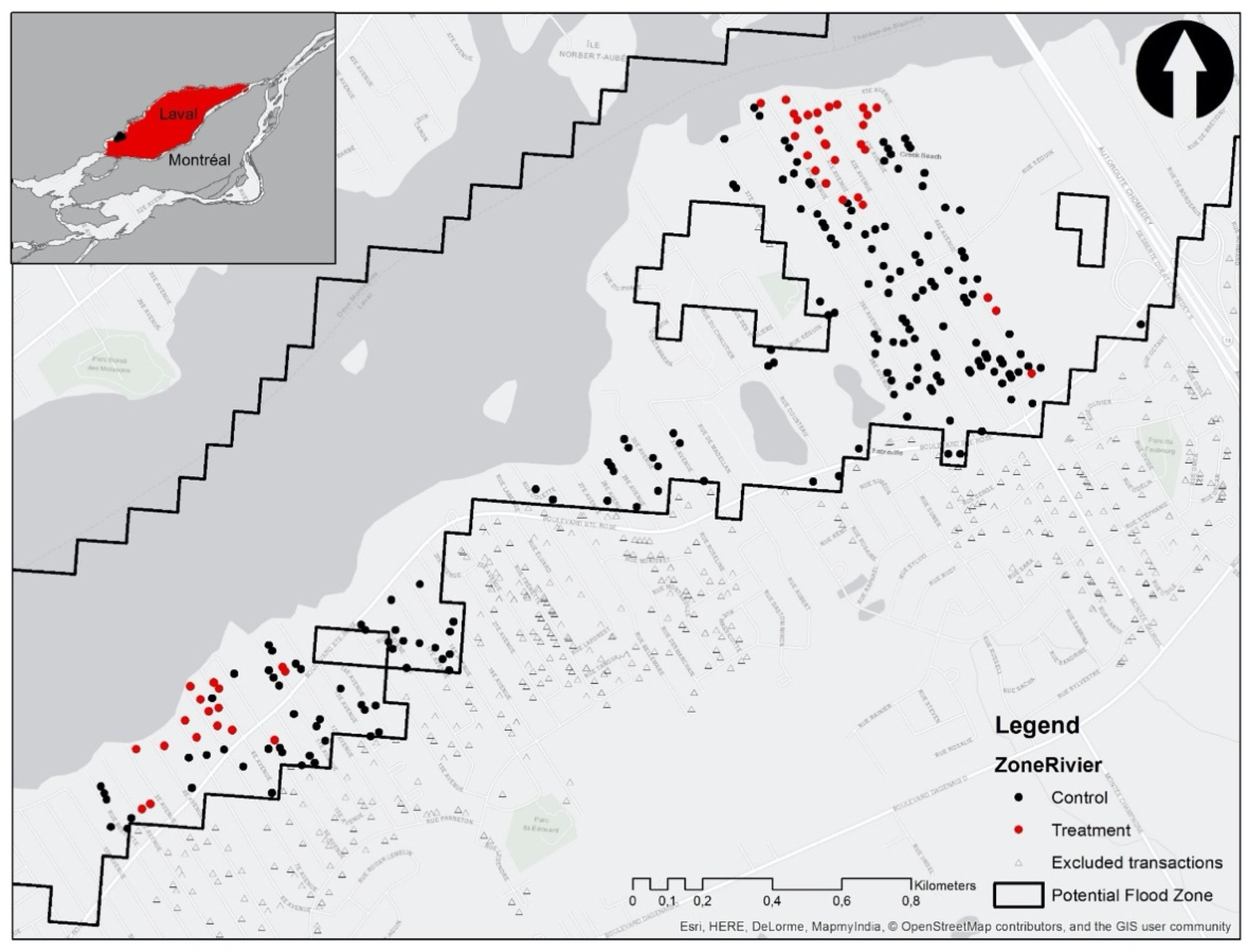
The methodological framework is applied to a flood event that occurred at the beginning of April 1998 in the city of Laval. Laval is an island which lies in the southwest of the province of Quebec (Canada) and is located to the north of the island of Montréal. It represents the largest of the Montreal suburbs. According to Statistics Canada Census of 2016, the city of Laval has a land area of 247.23 square kilometers and a population of 422,993. The island is separated from the surrounding territory by two rivers: the river Des Milles îles to the north, and the river Des Prairies to the south. The latter separates Laval island from the city of Montréal (Figure 2). Because of its specific geography, the island of Laval has been victim of flood events over time, but has been severely hit more recently, with major events occurring in the spring of 2017 and 2019.
The flood of 1998 was not strictly local. It evicted 3757 people from their houses in Quebec and Eastern Ontario according to the Montreal Gazette. Newspapers reported that at the time of the event, between 500 and 550 houses were affected by flooding in the city of Laval. This flood was qualified as a major event by the Public Security Agency (Ministère de la Sécurité Publique-MSP) and thus is considered to be one of the most important flood events to occur at that time.
Information on the precise location of the 1998 flood event is hard to obtain. While flood events are documented by the MSP, with information on the location and time of the event, the exact spatial delimitation of the flooded area is not precise. Available data provide information on the flooding zone, as defined by the local authority (Municipalité Régionale de Compté–or MRC). The zones are often imprecise and result in obtaining a delimitation of potentially flooded zones that are defined by the 0–20 year and 0–100 year probability. Thus, it is not because a house is located in this zone that it was necessarily flooded. A flooding zone only shows where floods are more likely to occur. Trying to isolate the impact based on this information can be misleading ([50]).
For the former reason, the authors use a proxy of the affected houses that is based on the precise delimitation of the houses that were ‘actually’ hit by more recent floods occurring during the spring of 2019. This new information, with good spatial coverage, is used as a proxy for where the flood of 1998 occurred. This proxy is based on satellite images localizing the floods and because the ground level is usually constant over short time periods, it is assumed that this information enables us to identify houses that are more likely to have faced flood events over time. This is assumed since natural disasters usually occur in the same place over time.
The empirical investigation is undertaken using single-family house transaction data for the city of Laval that occurred between 1995 and 2001 (i.e., three years before and after the flood). The total number of private dwellings in Laval is 165,686. The transaction data were purchased from the Greater Montreal Real Estate Board (GMREB). The original dataset consists of residential property transactions of single-family housing of a total number of 3469 observations located in the island of Laval in two districts: Fabreville and Sainte-Rose. Each observation represents information on the transaction price as well as the address which thus makes it possible to geocode property to its exact location (and coordinates) using GIS. Information on transactions includes a total of 15 descriptors for extrinsic and intrinsic amenities. Information on the characteristics of the neighborhood has been added to the database using census track for 1996 and 2001, resulting in 22 independent variables available for the analysis (Table 1).
Limiting the analysis to the neighborhood affected by the flood which is Fabreville, and identifying transactions occurring inside the potential flood zone (indicated by black points), with information on those that have more likely faced floods (indicated by red points), the total number of transactions for the analysis is 252 (Figure 2). Out of this number, 202 transactions lie inside the flooding zone (at risk) but did not face flood, 52 transactions are located inside the flooded zone, while 31 transactions occurred after the flood, i.e., after April 1998 (Table 2).
Without imposing any control for the amenities of the houses, prices appear to be statistically equal for houses that were likely hit by the flood (before and after the flood; p = 0.6817), while those potentially not hit have seen a significant rise in property value (p = 0.0112-Table 3). This quick comparison suggests that there could be a negative premium related to living inside the flood zone. However, the difference can be related to something else. Thus, there is a need to control for the structure of the houses to ensure that the difference is really related to the flood. This is what was further investigated in the analysis.
5. Results
The first step of the matching estimator with the spatial matching difference-in-differences (SM-DID) approach consists of developing a (logit) model to predict the probability of facing a flood (yes- Ds = 1-or no- Ds = 0-), i.e., receiving the treatment. This model has no particular meaning. It helps to identify the houses that have similar characteristics, as shown in the propensity score, based on the prediction of the probability of facing a flood event. It is not necessary to restrict the used variables to the “classical” amenities typically used in housing price models. It could also include other variables, such as the X and Y geographical coordinates. The addition of these variables helps to identify similar goods having similar locations and takes explicitly into account the spatial dimension.
The model estimated in this case shows an interesting prediction power, with a pseudo-R2 of 0.4787, and is globally significant (χ2 = 120.19; p = 0.0000). It also has a good specification, with a non-significant Hosmer & Lemeshow ([45]) statistic (p = 0.6171). The logit model has five (5) individual variables that appear to be statistically related to the location of the houses (Table 4).
To be useful, the prediction of the propensity score, based on the estimated model, needs to show a common support zone, which means that the model allows a common support zone (i.e., that the score of some houses located inside the zone is similar to those located outside the zone). To be interesting and useful, the counterfactuals need to be credible to adequately identify twins in both zones. Drawing the propensity score depending on the location (treatment or control) shows that the common support zone assumption holds.
Based on the predicted propensity score, the next steps consist of calculating the comparable sale prices of the twins. Using the neighbors inside the flood zone that were most likely not hit, it is possible to calculate the counterfactual sale price for those inside the zone and likely hit, and vice-versa. After having built the comparable price for both groups, it is possible to calculate the difference between the sale price depending on their location (Ds = {0,1}) and on the times when the transactions were recorded (Dτ = {0,1}).
The first difference, before the flood, shows a positive gap between the sale price for houses that were likely hit as compared to those that were not likely hit (Table 5). This first difference suggests a positive premium related to the proximity to the river, which is consistent with what economic theory suggests (i.e., houses with better amenities tend to be sold at higher prices). The second difference, after the flood, shows a negative difference for the same locations. This difference suggests that houses that were not likely hit were sold at higher prices than those that were likely hit (Table 5). The difference in the differences (DID) estimator shows a global negative effect on price varying between 18,000$ (for the two nearest neighbors) and 30,000$ (for one nearest neighbor). As the comparison based on only one neighbour is more sensitive to extreme values, the analysis focuses on the DID using between two and four neighbors. All results suggest similar impacts, i.e., a negative premium of the flood of about 20,000$ CAN.
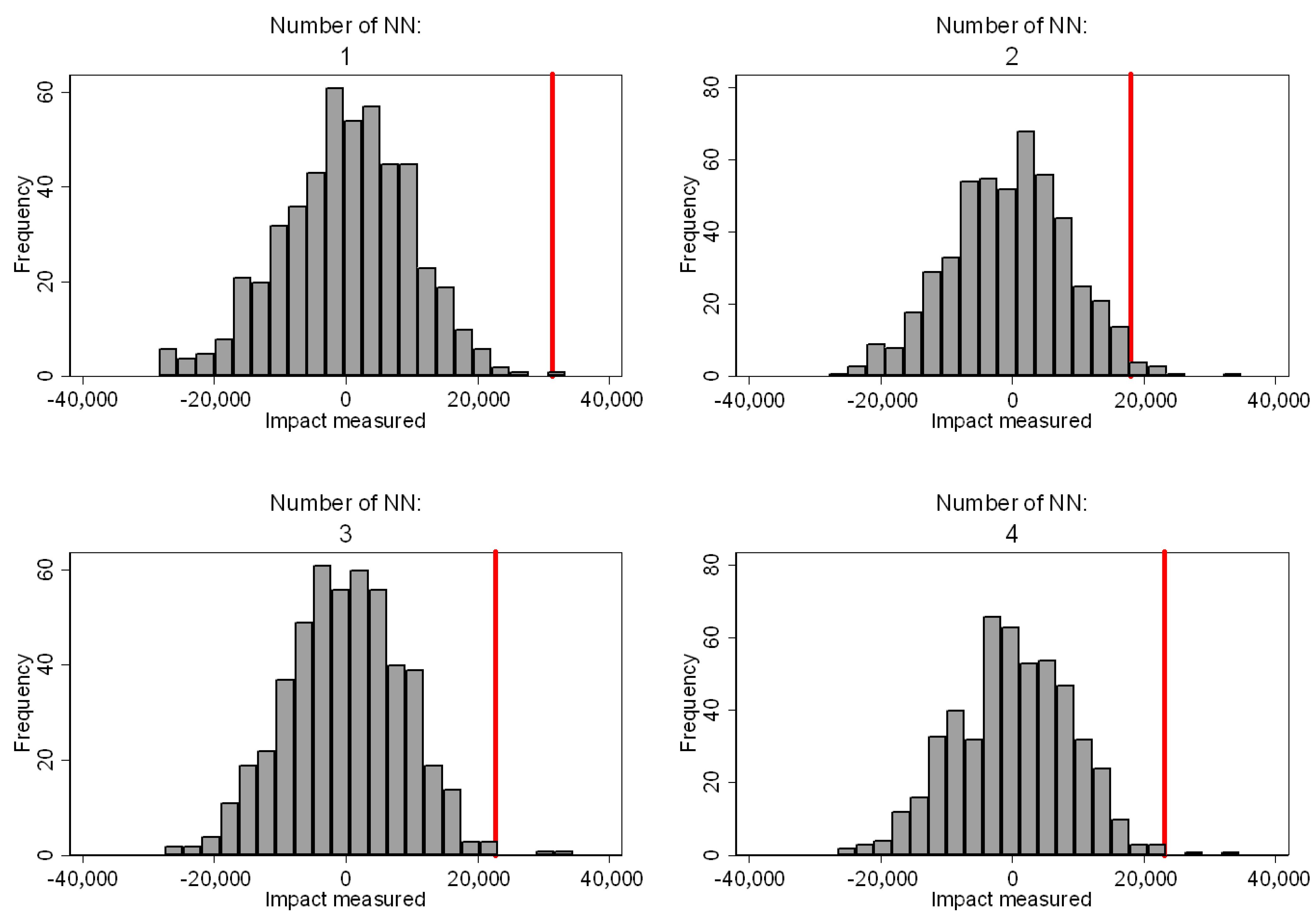
The analysis based on the falsification test confirms the significance of the noted difference (Figure 3). The fact that all results appear to be at the right end of the distribution confirms the robustness of the outcome. For all the used nearest neighbors, the analysis reveals that the impact measured using the dataset is different enough from what can be obtained based on a random assignation. Thus, the results are different from simple coincidence, which supports the conclusion and the significance of the impact.
6. Discussion
The impact of floods has long been discussed in the literature. However, their estimated impact remains highly heterogeneous. The fact that some studies find a positive effect of floods indicates that there are major drawbacks in the methodologies used in the evaluation of such impacts. The study shows that there is a need to adequately identify the zone that has really faced a flood. While many improvements have been suggested in recent work, such as the use of geographic regression discontinuity (GRD) analysis ([14,51]), limiting the analysis to the flooding zone, as is usually defined for 0–20 or 20–100 years, may not be accurate enough for such an exercise. Flood zones only help identify the risk of facing a flood, and not necessarily the fact that a flood has really occurred. Thus, the market tends to adjust to what has really occurred, and not to what can be a possible risk.
There is a need to work with more precise spatial information when one attempts to isolate the impact with spatial precision. The exact location of floods needs to be known when one is dealing with the estimation of their impact. Limiting the research to the large use of “potential flood zones” does not allow us to isolate the impact of floods that have really occurred since they are usually localized phenomena and are not systematically recorded in flooding zones. In fact, a flood zone can be used as a natural selection tool (for treatment and control zones) for comparing price changes for those houses that were flooded, compared to those that did not experience this drastic shock. There is a need to be spatially precise when one attempts to measure the impact of floods on housing prices. Otherwise, any outcome is possible.
The comparison based on the spatial matching difference-in-differences (SM-DID) estimator for a limited space is found to provide helpful insight for measuring and isolating the impact of a given event. Adopting a matching methodology limits the analysis to a local submarket and uses spatial delimitation which is proven to be advantageous and an interesting alternative to the hedonic pricing model. Firstly, it allows us to identify the difference before and after a flood event without using a sophisticated statistical model that may rely on an omission variable bias. Secondly, the intuition of the methodology is straightforward and can be seen as a natural extension of the professional practice based on the comparable sales approach. Thirdly, it is advantageous since it can be easily implemented on small datasets.
Of course, the proposed SM-DID methodological framework is not without possible drawbacks. The validity of the approach depends on the precision of the quality of adjustment of the logit model, as well as on the fulfillment of the common support zone assumption. Also, as is the case in many other empirical approaches, the proposed methodological framework faces challenges that are related to the construction of a good propensity score (or a general distance measure).
7. Conclusions
The paper proposes a new methodological framework for investigating the impact of an “exogenous” shock, such as a flood event, on housing prices. The proposed spatial matching difference-in-differences (SM-DID) estimator approach relies on an extension of the difference-in-differences (DID) estimator within a restricted area where the treatment and the control zones act as a dependent variable in a first stage. This approach allows us to adequately isolate the impact of environmental amenities and natural disasters, such as floods, while avoiding some drawbacks related to the classic price equation model of the hedonic pricing model (HPM). The methodological framework is a natural extension of the comparable sales approach (CSA) that is usually used in professional practice ([11]).
To test the methodological framework, an empirical investigation based on the 1998 flood that occurred in the city of Laval (Canada), which is a northern suburb of the city of Montréal, is presented. Using information on transactions occurring within a 0–20 year flood zone and information on houses that have been likely hit by floods inside this zone, (where houses hit by floods in 2019 were used as a proxy), the results suggest that floods have a negative impact on housing prices and reduce the sale price by about 20,000$ CAN.
The originality of the paper is two-fold. Firstly, the paper attempts to propose a new methodological framework and applies it to isolate the impact of flood on housing price. Secondly, it shows how empirical applications investigating the impact of flood events need to be adjusted to take into consideration the fact that being inside/outside a flooding zone is far from being sufficient to isolate the impact of such an environmental disaster. The work presented in this paper can easily be extended to any other evaluation of the impact of the extrinsic and external attributes of a real estate property as a complex good. The paper aims to provide an efficient way to isolate the impact of a given change (or an exogenous shock) on housing price without passing through the usual hedonic pricing model framework.
Of course, the application of the new methodological framework is not without challenges. The analysis largely depends on the appropriateness of the counterfactuals (or neighbors) identified to calculate the sale price of the comparable in the opposite group (treatment or control). The performance and the fit of the logit model (the first step) remain crucial in defining the counterfactuals, and researchers should pay careful attention to make sure that the investigation is adequate and that the impact is measured more precisely.
Author Contributions
Conceptualization, J.D. and M.A.; methodology, J.D.; software, M.A., J.D. and N.D.; validation, J.D. and N.D.; formal analysis, M.A. and J.D.; investigation, M.A.; resources, M.A., J.D. and N.D.; data curation, M.A.; writing—original draft preparation, M.A. and J.D.; writing—review and editing, J.D. and M.A.; visualization, J.D.; supervision, J.D.; project administration, J.D.; funding acquisition, J.D. All authors have read and agreed to the published version of the manuscript.
Funding
This research was funded by the Marine Environmental Observation, Prediction and Response Network (MEOPAR) by the project untitled “Comment passe-t-on à l’action avec les plans d’adaptation et de resilience? Projet de recherche en zone côtière et riveraine du Québec et de l’Ontario » under the supervision of Steve Plante (UQAR).
Institutional Review Board Statement
Not applicable
Informed Consent Statement
Not applicable.
Data Availability Statement
Not applicable.
Acknowledgments
The authors would like to thank Steve Plante.
Conflicts of Interest
The authors declare no conflict of interest.
Correction Statement
Due to an error in article production, several article preparation template sentences were included in the initial version of this publication. This information has been removed and the manuscript updated. This change does not affect the scientific content of the article.
References
- Verhoef, E.T.; Nijkamp, P. Externalities in the Urban Economy; Tinbergen Institute Discussion Paper No. 2003-078/3; Tinbergen Institute: Amsterdam, The Netherlands, 2003. [Google Scholar]
- Rosen, S. Hedonic Prices and Implicit Markets: Product Differentiation in Pure Competition. J. Political Econ. 1974, 82, 34–55. [Google Scholar] [CrossRef]
- Gibbons, S.; Machin, S. Valuing School Quality, Better Transport, and Lower Crime: Evidence from House Prices. Oxf. Rev. Econ. Policy 2008, 24, 99–119. [Google Scholar] [CrossRef]
- Dubé, J.; Thériault, M.; Des Rosiers, F. Commuter Rail Accessibility and House Values: The Case of the Montréal South Shore, Canada, 1992–2009. Transp. Res. Part A 2013, 54, 49–66. [Google Scholar] [CrossRef]
- Dubé, J.; Des Rosiers, F.; Thériault, M.; Dib, P. Economic Impact of a Supply Change in Mass Transit in Urban Areas: A Canadian Example. Transp. Res. Part A 2011, 45, 46–62. [Google Scholar] [CrossRef]
- Dubé, J.; Legros, D.; Thériault, M.; Des Rosiers, F. A Spatial Difference-in-Differences Estimator to Evaluate the Effect of Change in Public Mass Transit Systems on House Prices. Transp. Res. Part B 2014, 64, 24–40. [Google Scholar] [CrossRef]
- Kolak, M.; Anselin, L. A Spatial Perspective on the Econometrics of Program Evaluation. Int. Reg. Res. Rev. 2019, 43, 128–153. [Google Scholar] [CrossRef]
- Dubé, J.; Legros, D.; Thériault, M.; Des Rosiers, F. Measuring and Interpreting Urban Externalities in Real-Estate Data: A Spatiotemporal Difference-in-Differences (STDID) Estimator. Buildings 2017, 7, 51. [Google Scholar] [CrossRef]
- Antonakis, J.; Bendahan, S.; Jacquart, P.; Lalive, R. On Making Causal Claims: A Review and Recommendations. Leadersh. Q. 2010, 21, 1086–1120. [Google Scholar] [CrossRef]
- Kuminoff, N.V.; Pope, J.C. Do “Capitalization Effects” for Public Goods Reveal the Public’s Willingness to Pay? Int. Econ. Rev. 2014, 55, 1227–1250. [Google Scholar] [CrossRef]
- Yousfi, S.; Dubé, J.; Legros, D.; Thanos, S. Mass Appraisal without Statistical Estimation: A Simplified Comparable Sales Approach based on Spatiotemporal Matrix. Ann. Reg. Sci. 2020, 64, 349–365. [Google Scholar] [CrossRef]
- Sandink, D.; Kovacs, P.; Oulahen, G.; McGillivray, G. Making Flood Insurable for Canadian Homeowners; Discussion Paper; Institute for Catastrophic Loss Reduction and Swiss Reinsurance Company Ltd.: Toronto, ON, Canada, 2010. [Google Scholar]
- Jakob, M.; Church, M. The Trouble with Floods. Can. Water Resour. J. 2010, 36, 287–292. [Google Scholar] [CrossRef]
- Franco, S.F.; Macdonald, J.L. Living on the Edge: How Does Your House Price Respond to Urban Hazard Risk? Available online: https://economics.ucr.edu/wp-content/uploads/2019/10/Franco-paper-for-11-2-18-seminar.pdf (accessed on 6 June 2020).
- Rajapaksa, D.; Wilson, C.; Managi, S.; Hoang, V.; Lee, B. Flood Risk Information, Actual Floods and Property Values: A Quasi-Experimental Analysis. Econ. Rec. 2016, 92, 52–67. [Google Scholar] [CrossRef]
- Rajapaksa, D.; Wilson, C.; Hoang, V.; Lee, B.; Managi, S. Who Responds more to Environmental Amenities and Dis-amenities? Land Use Policy 2017, 62, 151–158. [Google Scholar] [CrossRef]
- Rajapaksa, D.; Zhu, M.; Lee, B.; Hoang, V.; Wilson, C.; Managi, S. The Impact of Flood Dynamics on Property Values. Land Use Policy. 2017, 69, 317–325. [Google Scholar] [CrossRef]
- Bin, O.; Landry, C. Changes in Implicit Flood Risk Premiums: Empirical Evidence from the Housing Market. J. Environ. Econ. Manag. 2013, 65, 361–376. [Google Scholar] [CrossRef]
- Bin, O.; Landry, C. Flood Hazards, Insurance Rate, and Amenities: Evidence from the Coastal Housing Market. J. Risk Insur. 2008, 75, 63–82. [Google Scholar] [CrossRef]
- West, T.L. Flood Mitigation and Response: Comparing the Great Midwest Floods of 1993 and 2008. Master’s Thesis, Naval Postgraduate School, Monterey, CA, USA, 2010. [Google Scholar]
- Montz, B.E. The Effects of Flooding on Residential Property Values in Three New Zealand Communities. J. Disaster Stud. Manag. 1992, 16, 283–298. [Google Scholar] [CrossRef] [PubMed]
- Eleuterio, J. Flood Risk Analysis: Impact of Uncertainty in Hazard Modelling Vulnerability Assessments on Damage Estimations. Ph.D. Thesis, University of Strasbourg, Strasbourg, France, 2012. [Google Scholar]
- Square One Insurance Services, Canadian Flood Maps: Is your Home in a Flood Zone. 2020. Available online: https://www.squareoneinsurance.com/resource-centres/home-personal-safety/canadian-flood-maps (accessed on 6 June 2020).
- Chruch, R.L.; Cova, T.J. Mapping Evacuation Risk on Transportation Network using a Spatial Optimization Model. Transp. Res. Part C 2000, 8, 321–336. [Google Scholar]
- Beltrán, A.; Maddison, D.; Elliott, R.J.R. Is Flood Risk Capitalized into Property Values? Ecol. Econ. 2017, 146, 668–685. [Google Scholar] [CrossRef]
- Beltrán, A.; Maddison, D.; Elliott, R.J.R. The Impact of Flood on Property Price: A Repeat-Sales Approach. J. Environ. Econ. Manag. 2019, 95, 62–86. [Google Scholar] [CrossRef]
- Atreya, A.; Ferreira, S. Seeing is Beleiving? Evidence from Property Prices in Inundated Areas. Risk Anal. 2015, 35, 828–848. [Google Scholar] [CrossRef] [PubMed]
- Atreya, A.; Ferreira, S.; Kriesel, W. Forgetting the Flood? An Analysis of the Flood Risk Discount over Time. Land Econ. 2013, 146, 668–685. [Google Scholar] [CrossRef]
- Bin, O.; Kruse, B. Real Estate Market Response to Coastal Flood Hazards. Nat. Hazards Rev. 2006, 7, 137–144. [Google Scholar] [CrossRef]
- Landry, C.; Hindsley, P.; Bin, O.; Kruse, J.B.; Whitehead, J.C.; Wilson, K. Weathering the Storm: Measuring Household Willingness-to-Pay for Risk-Reduction in Post-Katrina New Orleans. Mar. Resour. Econ. 2013, 28, 991–1013. [Google Scholar]
- Bin, O.; Polasky, S. Effects of Flood Hazards on Property Values: Evidence before and after Hurricane Floyd. Land Econ. 2004, 80, 490–500. [Google Scholar] [CrossRef]
- Kousky, C. Learning from Extreme Events: Risk Perceptions After the Flood. Land Econ. 2010, 86, 395–422. [Google Scholar] [CrossRef]
- Boyle, K.; Kiel, A. A Survey of House Price Hedonic Studies of the Impact of Environmental Externalities. J. Real Estate Lit. 2001, 9, 117–144. [Google Scholar]
- Ratcliffe, R. Valuation for Real Estate Decisions; Democrat Press: Washington, DC, USA, 1972. [Google Scholar]
- Colwell, P.F.; Cannaday, R.E.; Wu, C. The Analytical Foundations of Adjustment Grid Methods. Real Estate Econ. 1983, 11, 11–29. [Google Scholar] [CrossRef]
- Pace, R.K.; Giley, O.W. Generalizing the OLS and Grid Estimators. Real Estate Econ. 1998, 26, 331–347. [Google Scholar] [CrossRef]
- Des Rosiers, F.; Dubé, J.; Thériault, M. Hedonic Price Modelling: Measuring Urban Externalities in Québec. In Modelling Urban Dynamics: Mobility, Accessibility and Real Estate Value; Thériault, M., Des Rosiers, F., Eds.; ISTE-Wiley: London, UK, 2011; pp. 255–283. [Google Scholar]
- Cavailhès, J. Le prix des atttributs du logement. Écon. Stat. 2005, 381–382, 91–123. [Google Scholar]
- Huang, Z.; Chen, R.; Xu, D.; Zhou, W. Spatial and Hedonic Analysis of Housing Prices in Shanghai. Habitat Int. 2017, 67, 69–78. [Google Scholar] [CrossRef]
- Rodgers, T. Property-to-property Comparison. Apprais. J. 1994, 62, 64–67. [Google Scholar]
- Sheppard, S. Hedonic Analysis of Housing Markets. In Handbook of Regional and Urban Economics; Cheshire, P.C., Mills, E.S., Eds.; Elsevier: Amsterdam, The Netherlands, 1997; Volume 3, pp. 1595–1635. [Google Scholar]
- French, N.; Gabrielli, L. The Uncertainty of Valuation. J. Prop. Investig. Financ. 2004, 22, 484–500. [Google Scholar] [CrossRef]
- Rubin, D.B. Estimating Causal Effects of Treatments in Randomized and Nonrandomized Studies. J. Educ. Psychol. 1974, 66, 688–701. [Google Scholar] [CrossRef]
- Rosenbaum, P.R.; Rubin, D.B. The Central Role of the Propensity Score in Observational Studies for Causal Effects. Biometrika 1983, 70, 41–55. [Google Scholar] [CrossRef]
- Hosmer, D.W.; Lemeshow, S. A Goodness-of-fit Test for Multiple Logistic Regression Model. Commun. Stat. 1980, 9, 1043–1069. [Google Scholar] [CrossRef]
- Heβ, S. Randomization Inference with Stata: A Guide and Software. Stata J. 2017, 17, 630–651. [Google Scholar]
- Edgington, E.S. Randomization Tests, 2nd ed.; Marcel Dekker: New York, NY, USA, 1987. [Google Scholar]
- Onghena, P. Randomization and the Randomization Test: Two Sides of the Same Coin. In Randomization, Masking, and Allocation Concealment; Berger, V., Ed.; Chapman & Hall/CRC Press: Boca Raton, FL, USA, 2018; pp. 331–347. [Google Scholar]
- Anselin, L. Local Indicators of Spatial Association—LISA. Geogr. Anal. 1995, 27, 93–115. [Google Scholar] [CrossRef]
- AbdelHalim, M. Estimating Flood Impact on Residential Values (Housing Price): The Case of Laval (Canada). 1995–2007. Master’s Thesis, Université Laval, Québec, QC, Canada, 2020. [Google Scholar]
- Hidano, N.; Hoshino, T.; Sugiura, A. The Effect of Seismic Hazard Risk Information and Property Prices: Evidence from a Spatial Regression Discontinuity Design. Reg. Sci. Urban Econ. 2015, 55, 113–122. [Google Scholar] [CrossRef]
Figure 1.
Schematic Representation of a Spatial Matching Difference-in-Differences (SM-DID) Estimator.
Figure 1.
Schematic Representation of a Spatial Matching Difference-in-Differences (SM-DID) Estimator.

Figure 2.
Location of Flooded Transactions.

Figure 3.
Permutation Test Results. Note: Red Line → Estimation with matching; Histogram → Estimation with falsification. Each sub-figure use different number of nearest neighbours (1 to 4).
Figure 3.
Permutation Test Results. Note: Red Line → Estimation with matching; Histogram → Estimation with falsification. Each sub-figure use different number of nearest neighbours (1 to 4).


Table 1.
List of Variables Available for the Analysis.
| Variable Name | Source | Mean | s.d. |
|---|---|---|---|
| Age (in years) | GMREB | 19.833 | 16.840 |
| Lot size (in m2) | GMREB | 5430.186 | 2495.990 |
| Garage (Yes/No) | GMREB | 0.369 | 0.484 |
| Basement (Yes/No) | GMREB | 0.353 | 0.479 |
| Excavated pool (Yes/No) | GMREB | 0.052 | 0.222 |
| Bungalow (Yes/No) | GMREB | 0.556 | 0.498 |
| Multi-storey House (Yes//No) | GMREB | 0.067 | 0.251 |
| Cottage (Yes/No) | GMREB | 0.377 | 0.486 |
| Semi-detached house (Yes/No) | GMREB | 0.171 | 0.377 |
| Being inside 0–20 years flooding zone (Yes/No) | Données Quebec | 0.175 | 0.380 |
| X coordinates (in meters-NAD83) | GMREB | 277,713 | 783.344 |
| Y coordinates (in meters-NAD83) | GMREB | 5,047,705 | 671.178 |
Note: GMREB → Greater Montreal Real Estate Board; NT = 252 observations; s.d. → Standard deviation.
Table 2.
Transactions According to Their Status.
| Flood Event | |||
|---|---|---|---|
| Treatment | Before (Dτ = 0) | After (Dτ = 1) | Total |
| Outside the zone (Ds = 0) | 67 | 135 | 202 |
| Inside the zone (Ds = 1) | 19 | 31 | 50 |
| Total | 86 | 166 | 252 |
Table 3.
Descriptive Statistics for Houses Inside and Outside (Ds) the Flood Zone, Before and After (Dτ) the Treatment.
Table 3.
Descriptive Statistics for Houses Inside and Outside (Ds) the Flood Zone, Before and After (Dτ) the Treatment.
| Main Statistics | |||
|---|---|---|---|
| Final Sale Price (in $) | N | Mean | s.d. |
| All Transactions | 252 | 85,938 | |
| Outside the zone (Ds = 0) | 202 | 88,544 | 1873 |
| Before (Dτ = 0) | 67 | 81,825 | 2837 |
| After (Dτ = 1) | 135 | 91,878 | 2379 |
| Inside the zone (Ds = 1) | 50 | 75,411 | 4496 |
| Before (Dτ = 0) | 19 | 73,021 | 7468 |
| After (Dτ = 1) | 31 | 76,876 | 5706 |
Table 4.
Estimated Logit Model (Coefficients and Statistical Significance).
| Variables | Coefficient | Sign |
|---|---|---|
| Age (in years) | −0.0057 | |
| Lot size (in m2) | 0.0002 | |
| Garage (Yes/No) | −1.1927 | ** |
| Basement (Yes/No) | 0.5856 | |
| Excavated pool (Yes/No) | 0.1517 | |
| Bungalow (Yes/No) | Reference | |
| House with many storeys (Yes//No) | −2.4311 | ** |
| Cottage (Yes/No) | −1.3012 | ** |
| Town house: Semi-detached house (Yes/No) | −0.3114 | |
| Within a restrained flooding zone (Yes/No) | 3.5358 | *** |
| X coordinates (in meters-NAD83) | −0.0046 | *** |
| Y coordinates (in meters-NAD83) | 0.0044 | *** |
| Constant | −20,825.51 | *** |
| Pseudo-R2 | 0.4787 | |
| χ2-stat | 120.19 | *** |
| Hosmer-Lemeshow stat | 6.27 |
NT = 252; Legend: *** p < 0.01; ** p < 0.05.
Table 5.
List of Variables Available for the Analysis.
| ZIS Zone | ||||
|---|---|---|---|---|
| # of NN | Before | After | DID | Sign |
| 1 | 1,373,895 | −1,756,850 | 3,130,745 | *** |
| 2 | 1,614,360 | −179,040 | 1,793,400 | *** |
| 3 | 2,236,182 | −27,450 | 2,263,632 | *** |
| 4 | 1,455,233 | −859,761 | 2,314,994 | *** |
Note: NN is nearest neighbors; Legend: *** p < 0.01.
Publisher’s Note: MDPI stays neutral with regard to jurisdictional claims in published maps and institutional affiliations. |
© 2021 by the authors. Licensee MDPI, Basel, Switzerland. This article is an open access article distributed under the terms and conditions of the Creative Commons Attribution (CC BY) license (http://creativecommons.org/licenses/by/4.0/).
Share and Cite
MDPI and ACS Style
Dubé, J.; AbdelHalim, M.; Devaux, N. Evaluating the Impact of Floods on Housing Price Using a Spatial Matching Difference-In-Differences (SM-DID) Approach. Sustainability 2021, 13, 804. https://0-doi-org.brum.beds.ac.uk/10.3390/su13020804
AMA Style
Dubé J, AbdelHalim M, Devaux N. Evaluating the Impact of Floods on Housing Price Using a Spatial Matching Difference-In-Differences (SM-DID) Approach. Sustainability. 2021; 13(2):804. https://0-doi-org.brum.beds.ac.uk/10.3390/su13020804
Chicago/Turabian StyleDubé, Jean, Maha AbdelHalim, and Nicolas Devaux. 2021. "Evaluating the Impact of Floods on Housing Price Using a Spatial Matching Difference-In-Differences (SM-DID) Approach" Sustainability 13, no. 2: 804. https://0-doi-org.brum.beds.ac.uk/10.3390/su13020804
Note that from the first issue of 2016, this journal uses article numbers instead of page numbers. See further details here.