Modeling and Simulation of a Proton Exchange Membrane Fuel Cell Alongside a Waste Heat Recovery System Based on the Organic Rankine Cycle in MATLAB/SIMULINK Environment

Abstract

The proton exchange membrane fuel cell (PEMFC) is the fastest growing fuel cell technology on the market. Due to their sustainable nature, PEMFCs are widely adopted as a renewable energy resource. Fabricating a PEMFC is a costly process; hence, mathematical modeling and simulations are necessary in order to fully optimize its performance. Alongside this, the feasibility of a waste heat recovery system based on the organic Rankine cycle is also studied and power generation for different operating conditions is presented. The fuel cell produces a power output of 1198 W at a current of 24A. It has 50% efficiency and hence produces an equal amount of waste heat. That waste heat is used to drive an organic Rankine cycle (ORC), which in turn produces an additional 428 W of power at 35% efficiency. The total extracted power hence stands at 1626 W. MATLAB/Simulink R2016a is used for modeling both the fuel cell and the organic Rankine cycle.

1. Introduction

Due to the advancements in technology, the use of fuels of various types has increased tenfold. Therefore, human beings are using fossil fuels (oil, gas and coal) to fulfill their daily energy requirements. This has led to the depletion of such resources. Even though new reserves are being discovered, burning of fossil fuels presents another major problem. Combustion of fossils fuels results in the emission of carbon dioxide (CO₂), which gives rise to the greenhouse effect. CO₂ emissions increased by 1.5% in 2018 [1]. The greenhouse effect causes the temperature of the Earth to increase and this results in global warming. Global warming is a major issue that is resulting in the melting of the polar ice caps. The ever-increasing sea level can cause tsunamis and flooding in coastal areas. Due to this environmental pollution, the need for clean and substantial energy is required because the demand for electricity and energy is increasing globally due to the increasing population. In order to minimize the damage that is being done to our environment, the world has started moving towards alternative sources of energy. Renewable energy resources are the most clean and green source of energy. In the last decade, much advancement has been made in renewable energy technologies, such as solar, wind, and tidal, etc. The only drawback of renewable energy is that it is dependent upon external factors, such as solar irradiation, wind velocity, etc. These external factors cannot be controlled and are entirely dependent upon nature. An alternative resource for producing clean energy is the use of fuel cells. Fuel cells are the perfect solution for meeting the everlasting energy requirement [2]. They can also be used as a fuel source for unmanned vehicles due to their compact and easy to refuel nature [3]. A similar study on the comparison between lead acid, lithium, and fuel cells for use in unmanned vehicles was performed in [4]. Fuel cells do not depend upon weather conditions and they do not produce any pollution or harmful gases. Researchers are working on reducing their production cost to make them commercially affordable.

1.1. Fuel Cell Technology

Fuel cells are devices that perform on the principle of electrochemistry. In fuel cell systems, the polymer electrolyte membrane fuel cells (PEMFC) is one of the most significant technologies that have been discovered. Researchers are investigating this technology very carefully, as it is a safe, clean, and efficient energy source. Studies have shown that PEMFCs have longer lifetimes and cost much less than other fuel cell technologies [5]. Polymer electrolyte membrane fuel cells (PEMFCs) are the most preferred type of fuel cell due to their high power density, low operating temperature, and high conversion efficiency of 50–60%, and they have zero emission potential into the environment when pure hydrogen is utilized [6,7].

Experimental implementation is very costly for fuel cells due to the complexity of their design [8,9]. In this case, simulation models of fuel cells generated in software play a significant role in research development. Simulation models of fuel cells are basically used to carry out simulations of models practically. This makes it easier for researchers to study the parameters that influence the functioning of a fuel cell. These simulations are making the development of fuel cells easier for researchers and are also reducing the cost of experimental implementation. Another advantage of simulations is that they save time. Fabricating a fuel cell system and then studying the response by varying parameters would be costly, time consuming, and complex. On the other hand, one can study all the parameters on software easily.

Researchers are constantly working on improving the performance of fuel cells. Wang et al. [10] discussed the development of PEMFC technology over the years. The current status of PEMFC technology is that it is mostly being used in transportation applications, such as lightweight vehicles, buses, etc. Francesconi et al. [11] analyzed the behavior of a fuel cell by varying parameters such as fuel cell temperature, pressure etc. Hydrogen was reformed to produce ethanol, which was used as the fuel. It was concluded that pressure has a key impact on the performance of the fuel cell.

Li et al. [12] discussed the use of PEMFCs in high temperature environments. The membrane of a PEMFC can be modified with an acid-base polymer to make it operational at elevated temperatures, from 100 to 200 °C.

The dynamic modeling of fuel cells has been extensively studied by researchers. Azri et al. [13], based on an equivalent electric circuit of a PEMFC, developed steady-state, dynamic, and thermodynamic models and used MATLAB to investigate a Horizon H-500 fuel cell stack. Different PEMFC parameters such as power output, stack voltage, etc., were analyzed. First, the activation, ohmic, and concentration losses were studied using a steady-state model. Then, a dynamic model was developed to visualize dynamic voltage and dynamic power parameters of PEMFC by considering double layer charging effect which acts as a capacitor in the electric circuit. The thermodynamic model was used to visualize the effect of temperature inside a fuel cell. The results from his work show that only the ambient temperature and gas pressure of the inlet affects the performance of a PEMFC. Benchouia et al. [14] analyzed the steady-state and dynamic behavior of a PEMFC. Validation of the results was carried out by comparing simulation results with an experimental fuel cell stack.

Valencia et al. [15] also carried out research on a three-dimensional numerical study of heat transfer in PEMFC. Computational fluid dynamics (CFD) was used to solve governing equations. In their work, they obtained distribution contours of temperature distribution throughout the fuel cell. It was also found that the anode compartment has a lower temperature than the cathode compartment. It was demonstrated that there exists a direct relation between the temperature and current density of a fuel cell. It was found that heat produced from ohmic losses and electrochemical reactions is removed through ta convection process via channels, and these channels, when used in parallel, help to remove heat from the fuel cell. From this work, information for heat transfer processes was obtained that can be used to optimize designs of PEMFC.

Santarelli et al. [16] described the process of estimating some operating parameters of PEMFC. First, the main parameters, such as limiting current density, internal current density, exchange current density and cell resistance, were analyzed. Later, a model to discuss the polarization curve was developed. Parameter analysis was performed in the model and it was demonstrated that three parameters of the polarization curve can be estimated at the same time, namely internal current density, cathode exchange current density, and cell resistance. In the model, the temperature of the cell was varied from 50 to 80 °C, and the behavior of parameters at each operating condition of cell was analyzed. The behavior of the polarization curve against the operating temperature was developed.

Xue et al. [17] analyzed the steady-state and dynamic modeling of a PEMFC based on the least squares techniques. The ideal voltage and ohmic loss equations were based on steady-state models, while the concentration and activation losses were based on dynamic losses. An optimized model of the fuel cell was generated.

Zhao et al. [18] studied the working of a PEMFC with transient characteristics. Their paper analyzed the working of a PEMFC under dynamic conditions such as different step currents. The dynamic response of a PEMFC was studied under stacking conditions.

1.2. Heat Recovery from Fuel Cells

Since fuel cells are not 100% efficient, the energy that is not converted into power is lost in the form of heat. This excess energy can be utilized in order to run another independent system. Heat recovery from fuel cells is another way to maximize their use and to increase their efficiency.

Lin et al. [19] analyzed the use of heat recovery systems in fuel cells. Three uses of heat recovery were stated in the paper,

• Fuel reforming process by the use of heat recovered from a fuel cell. Methanol or other hydrocarbons can undergo reforming in order to produce pure hydrogen (H₂), which can be utilized as a fuel for the PEMFC itself or for other systems.
• The use of a gas turbine working on the heat recovered from a high-temperature fuel cell such as a Solid Oxide Fuel Cell (SOFC) that operates at 800 to 1000 °C.
• The use of combined heat and power production system for residential neighborhoods. A fuel cell can generate both electricity, by electrochemical reaction, and heat, by excess heat losses, for indoor heating.

Yiding Cao [20] suggested a combination of a throttling valve, heat exchanger and other components in order to recover heat from a fuel cell. He concluded that the efficiency of a fuel cell power plant can be improved by 20% by installing a heat recovery system.

Vikrant Venkataraman [21] analyzed the working of a vapor absorption cycle (VAC) working on the heat recovered from a SOFC. The major problem was the temperature difference between the two systems. Direct and indirect coupling was used in order to transfer heat from the SOFC to the VAC at the right temperature.

Michel Fuchs [22] designed a model to incorporate an ejector refrigeration cycle into a high temperature PEMFC. A new method of using the waste heat of a fuel cell was analyzed, which increased the overall efficiency of the fuel cell.

Guo et al. [23] studied the integration of a vapor absorption cycle working on the principle of heat recovery from a high-temperature PEMFC. The absorption cycle was used as both a heat pump and a refrigeration cycle. The power densities for both scenarios were analyzed.

2. Materials and Methods

In order to simulate a working model of a PEMFC, it is necessary to understand the basic working behind the fuel cell.

2.1. Fundamentals of a PEMFC

A fuel cell consists of three main components:

• An electrode for fuel (anode)
• An electrode for oxygen (cathode)
• Electrolyte between cathode and anode

The electrode is made from a porous material that is combined with platinum. The porous electrode allows the gases to pass through it.

The working of the fuel cell [24] is explained. The hydrogen (H₂) is introduced into the fuel cell by the fuel inlet port. The hydrogen reaches the anode and reacts under the influence of platinum catalyst. The molecular hydrogen is broken into two protons (H⁺) as well as two electrons (e⁻). The electrons flow from the outer circuit, resulting in the flow of current. The protons penetrate across the acidic electrolyte in order to get to cathode.

Anode: H₂ (g) → 2H⁺ + 2e⁻

On the cathode, injection of oxygen takes place through the air inlet port. The electrons from the outer circuit bind with the protons and molecular O₂ in order to produce water.

Cathode: (1/2) O₂ (g) + 2H⁺ + 2e⁻→ H₂O

(1)

The overall reaction of the system can be written as

Overall reaction: H₂ (g) + (1/2) O₂ (g) → H₂O

(2)

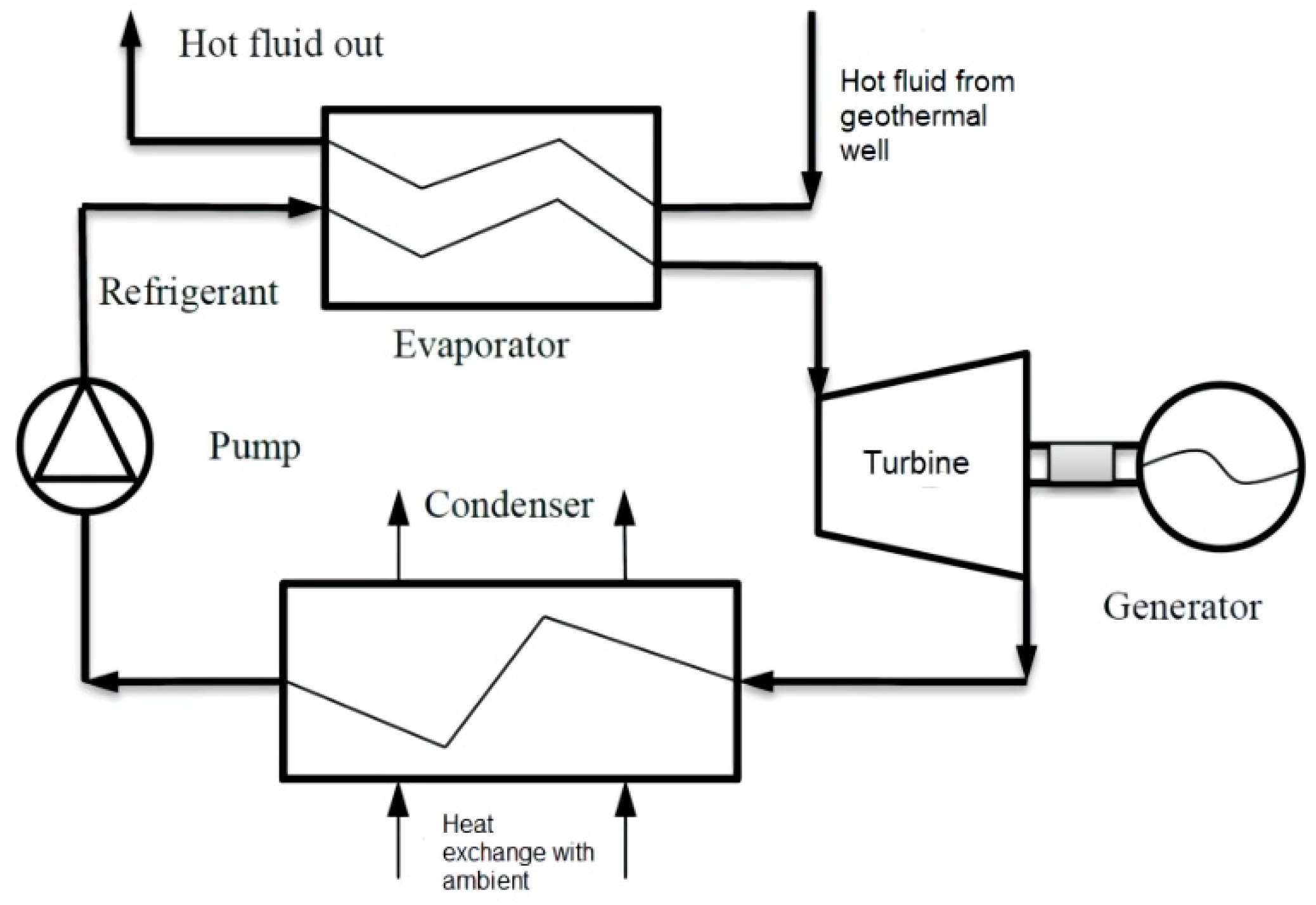
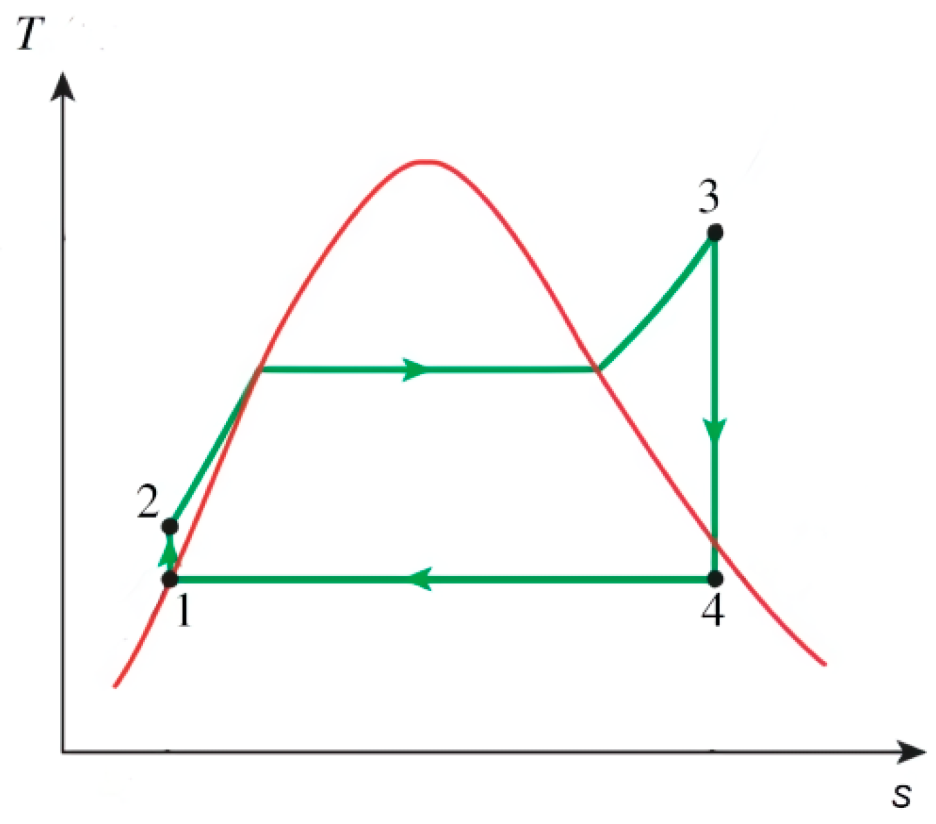
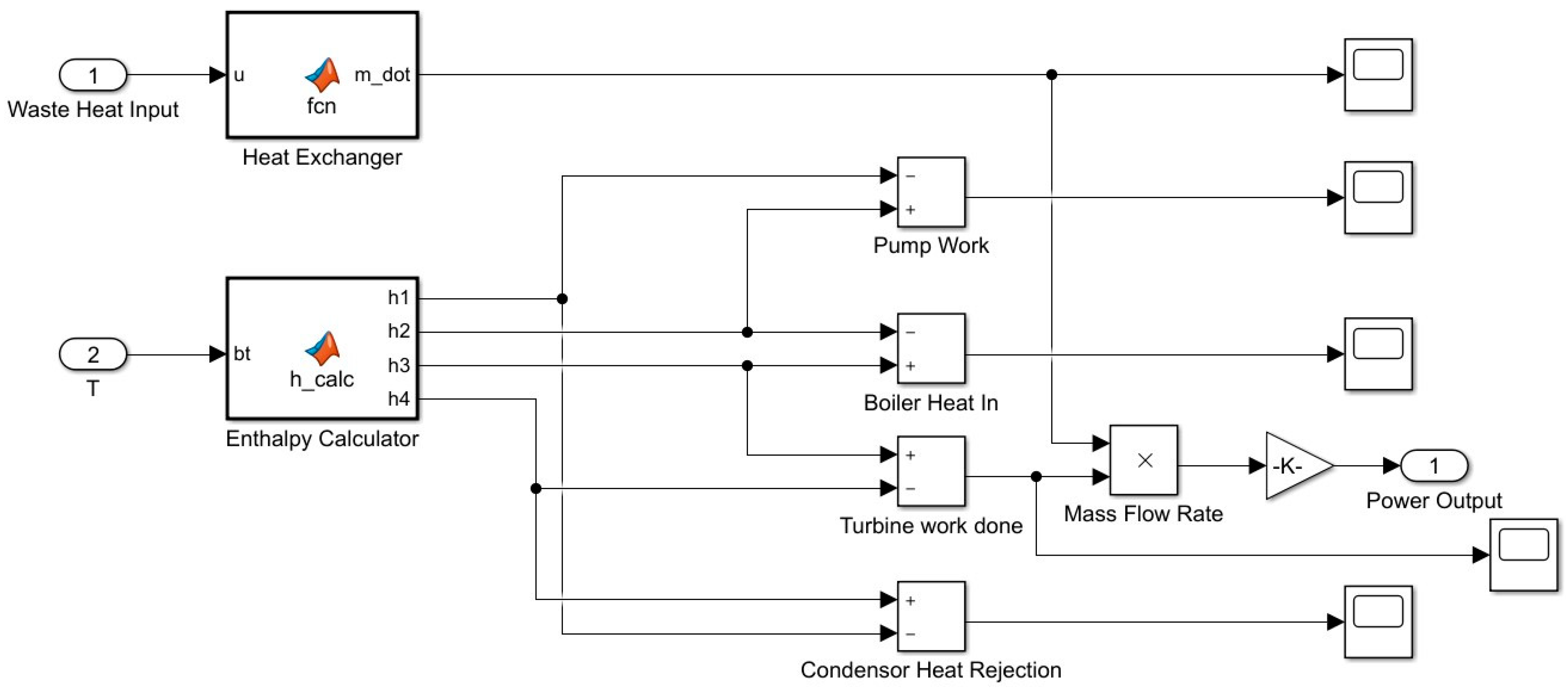
2.2. Fundamentals of an Organic Rankine Cycle (ORC)

Organic Rankine Cycle

The organic Rankine cycle (ORC) is the preferred thermodynamic cycle that is used for power generation by using a low-temperature heat source. Since the PEMFC operates at a low temperature range of 80 to 100 °C, using an ORC makes sense. The cooling fluid for the fuel cell directly enters the ORC as its working fluid. Heat and pressure losses for this fluid will be neglected for simplicity. [25]. The cycle performs in a similar manner to a Rankine cycle. The difference arises in the working fluid. A Rankine cycle uses water as the working fluid, which can be vaporized into steam inside the boiler at a certain temperature and pressure. Unlike the Rankine cycle, an ORC utilizes a zeotropic mixture as the working fluid. The zeotropic mixture has the ability to vaporize at a much lower temperature as compared to water. Hence, it is useful for operating at a lower temperature.

The organic Rankine cycle operates on a similar principle as the Rankine cycle. The main purpose of the cycle is to utilize the thermal energy of the working fluid and convert it into the kinetic energy of superheated vapor. This superheated vapor has a high pressure and temperature, and its energy can be used to rotate the turbine as it expands.

The ORC, shown in Figure 1, contains the same components as the Rankine cycle. The cycle begins at the pump where the working fluid arrives as a saturated liquid. The pump compresses it isentropically and raises its pressure to the working pressure of the evaporator. Since the specific volume of fluid decreases, the temperature of the fluid increases slightly. After being pumped to a higher pressure, the fluid enters the evaporator. This component in a Rankine cycle is known as a boiler, where water is heated in order to vaporize it into superheated steam. For an ORC, an evaporator is used. The evaporator acts as a heat exchanger and helps in transferring heat from the hot source to the working fluid. In this paper, the heat from the hot source is gained from the hot fluid coming out of a PEMFC. This hot fluid is made to flow through the evaporator, where it exchanges heat with the working fluid of the ORC. The fluid then vaporizes and converts into a superheated state with a high pressure and temperature.

This superheated vapor is then sent to the turbine, where it undergoes expansion isentropically. This expansion causes the turbine blades to rotate. The turbine is connected to a generator which produces electricity. The expansion of the fluid results in a drop in its temperature and pressure.

At this stage, the fluid enters the condenser. The fluid, at this point, can be a saturated liquid–vapor mixture with a high-quality value. The condenser acts as a heat exchanger that exchanges heat with a sink. The sink is at a lower temperature than the condenser. The condenser rejects heat to the sink, resulting in the cooling of the working fluid. The fluid exits the condenser as a saturated liquid and the cycle starts again.

The organic Rankine cycle can be summarized as follows:

• Isentropic compression (pump)
• Constant pressure heat addition (evaporator)
• Isentropic expansion (turbine)
• Constant pressure heat rejection (condenser)

3. Results

Modeling of a PEMFC model in a MATLAB/SIMULINK environment requires certain equations for steady-state and dynamic models. Using these equations, a model can be developed to test the response of the PEMFC by varying certain input parameters. In this paper, the modeling is done on Horizon H-500 Fuel Cell parameters.

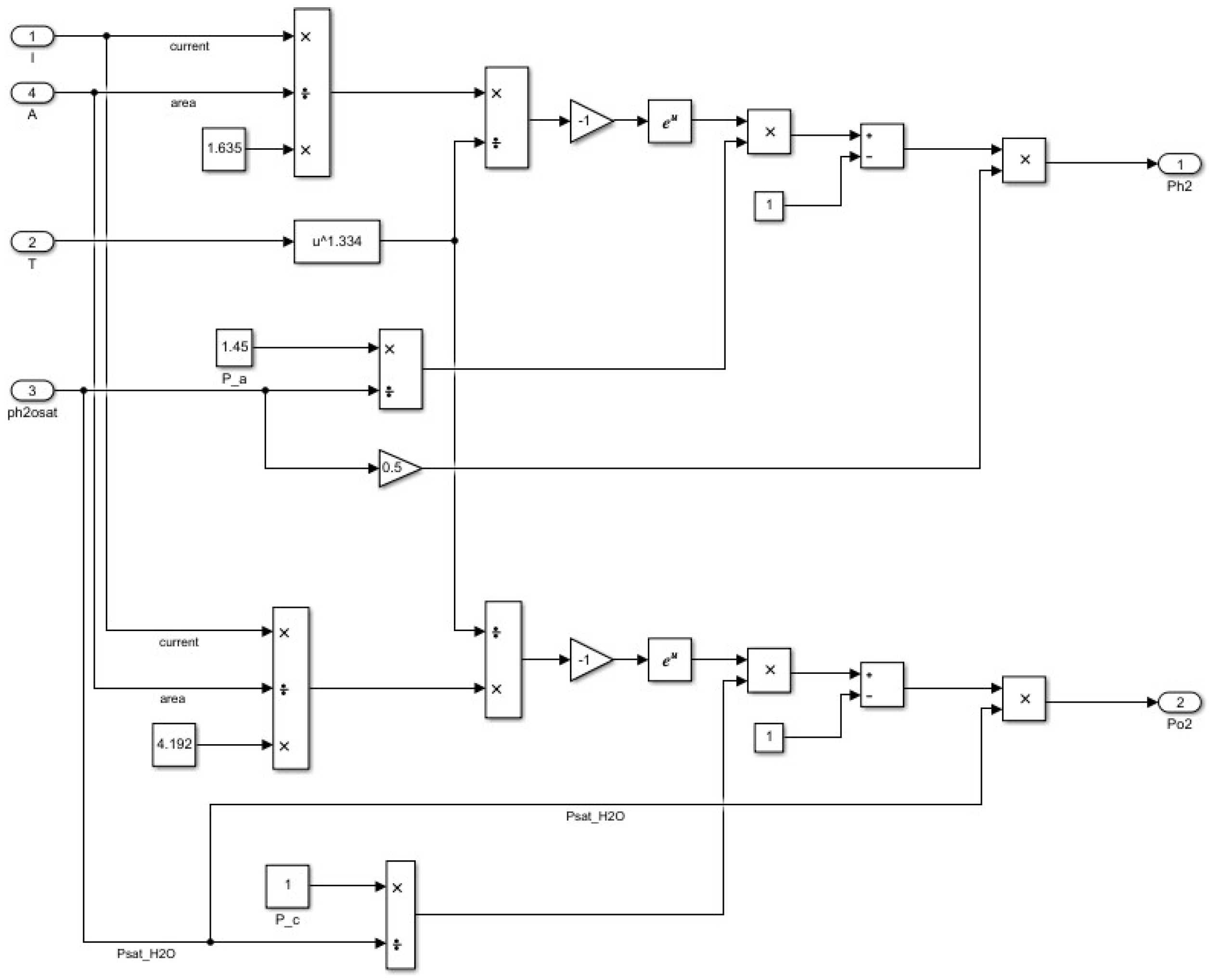
3.1. Steady-State Modelling

Figure 2 shows the response of a single cell of a PEMFC against varying current density. The straight horizontal line at the top represents the ideal voltage of the PEMFC. The ideal voltage occurs during the open-circuit condition, i.e., when there is no current passing across the outer circuit of the fuel cell. The ideal voltage of a fuel cell can be represented by the Nernst Equation (3):

$$E= E^0-\frac{RT}{2F}\ln \left(P_{H_2}\ast P_{O_2}{}^{0.5}\right)$$

(3)

where E⁰ is the EMF at standard pressure and is also known as the ideal cell voltage. E⁰ is typically taken as 1.229 V when the output of the PEMFC is liquid H₂O and 1.8 V when the product is gaseous H₂O [27]. E is the potential at the thermodynamic equilibrium. R (Universal gas constant, 8.314 J·mol⁻¹·K⁻¹) and F (Faraday’s Constant, 96,485) are constants, whereas 2 represents the number of electrons flowing through the outer circuit. The temperature of the PEMFC is denoted by T, represented in Kelvin (K). PH₂ and PO₂ are the partial pressures of the hydrogen (fuel) and oxygen (air) at the anode and cathode, respectively.

The equation for ideal voltage can then be simplified by substituting all the constants and by expansion:

$$E= 1.229-8.5e^{-4}\left(T_{cell}-298.15\right)+4.308e^{-5}\left[\ln \left(P_{H_2}\right)+0.5\ln \left(P_{O_2}\right)\right]$$

(4)

Partial pressures can be represented as:

$$P_{H_2}=0.5P_{H2O}{}^{sat}\left[\exp \left(-\frac{1.635J}{T_{cell}{}^{1.334}}\right)\left(\frac{P_a}{P_{H2O}{}^{sat}}\right)-1\right]$$

(5)

$$P_{O_2}=P_{H2O}{}^{sat}\left[\exp \left(-\frac{4.192J}{T_{cell}{}^{1.334}}\right)\left(\frac{P_c}{P_{H2O}{}^{sat}}\right)-1 \right]$$

(6)

where:

• P_a = partial pressure at anode
• J = current density
• P_c = partial pressure at cathode
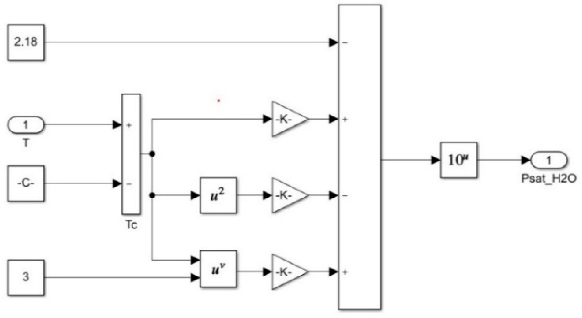
• P_H2O ^sat = saturation pressure of water

$$lo{g}_{10}{P}_{H2O}{}^{sat}=-2.18+2.95e^{-2}{T}_c-9.18e^{-5}{T}_c{}^2+1.44e^{-7}{T}_c{}^3$$

(7)

$$T_c= T_{cell}-273.15$$

(8)

The final voltage generated by the fuel cell is the sum of the ideal voltage and three losses. These losses occur during three different stages, as shown in Figure 3. These three losses are now discussed in detail.

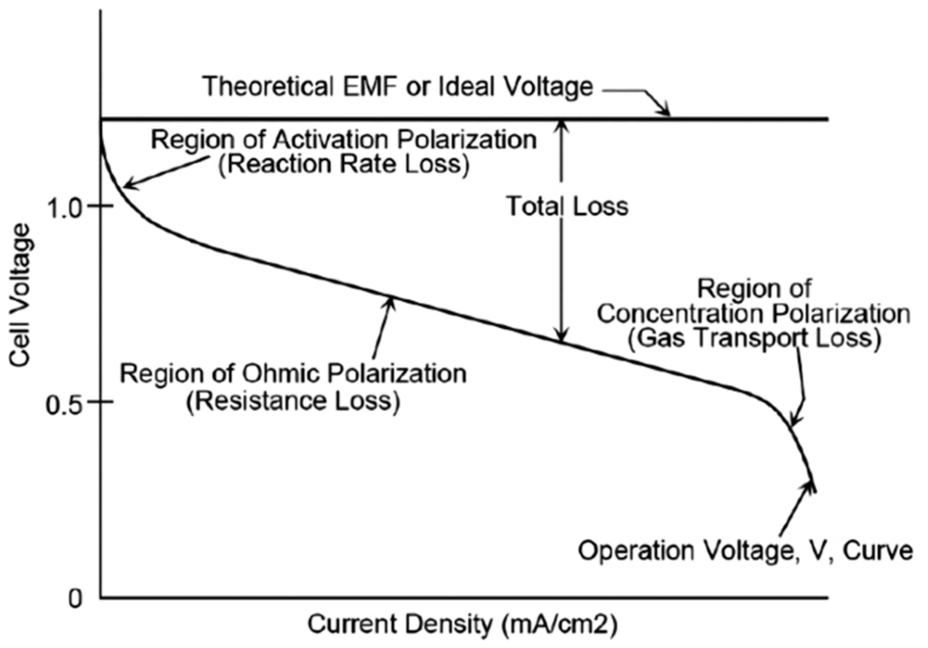
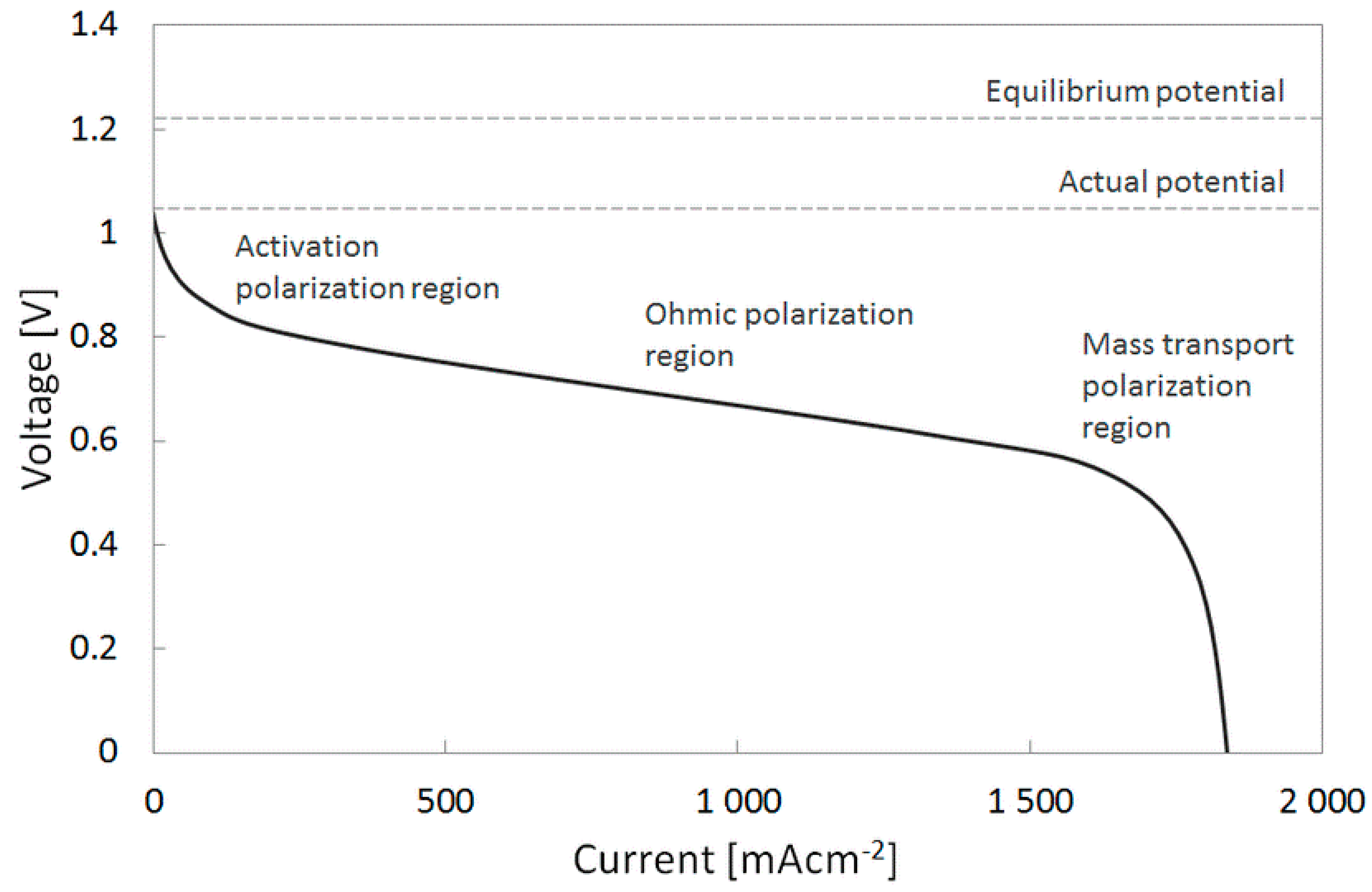
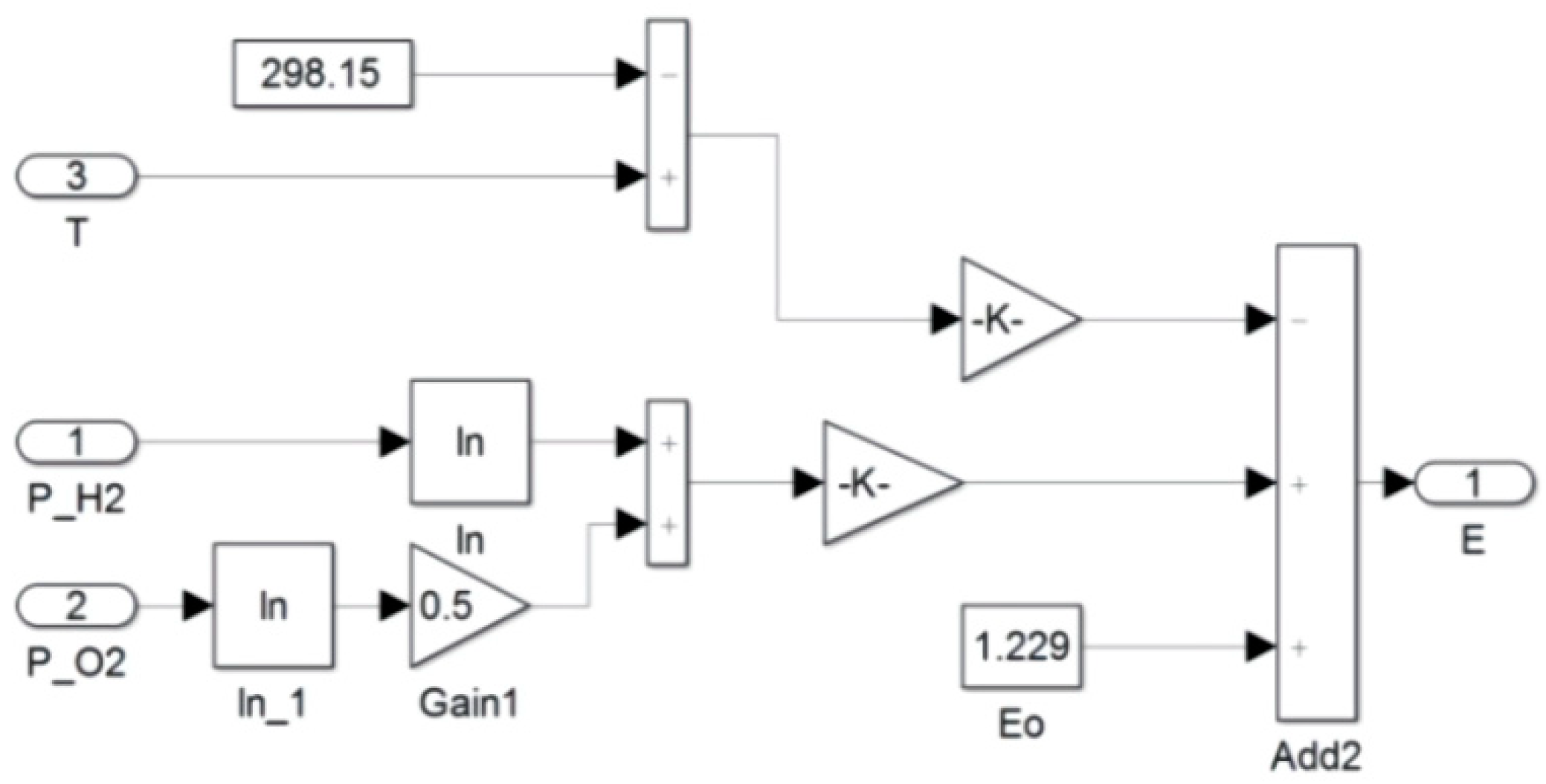
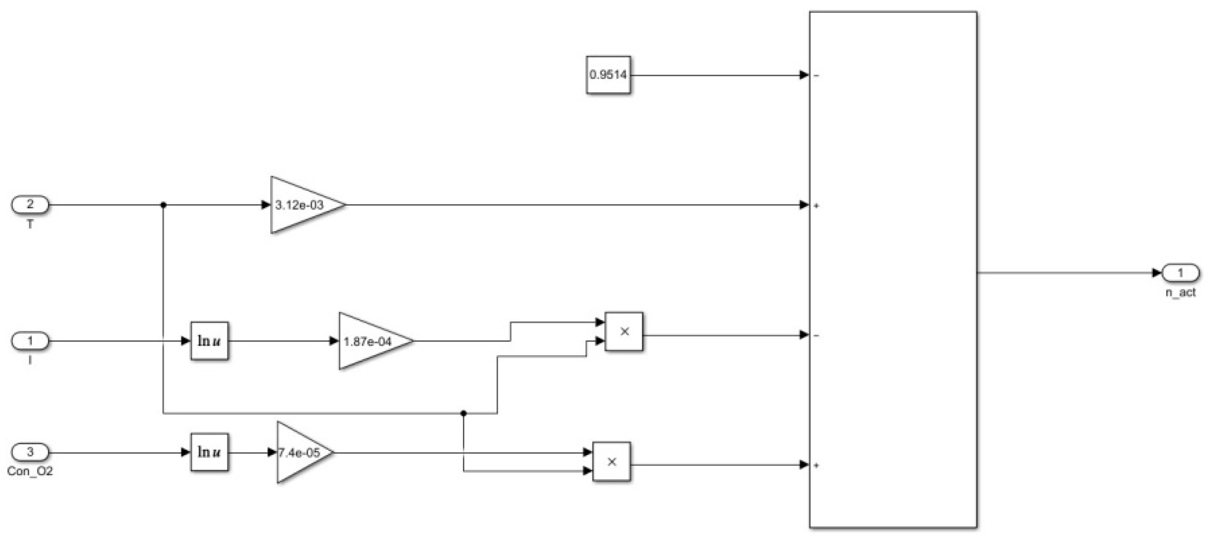
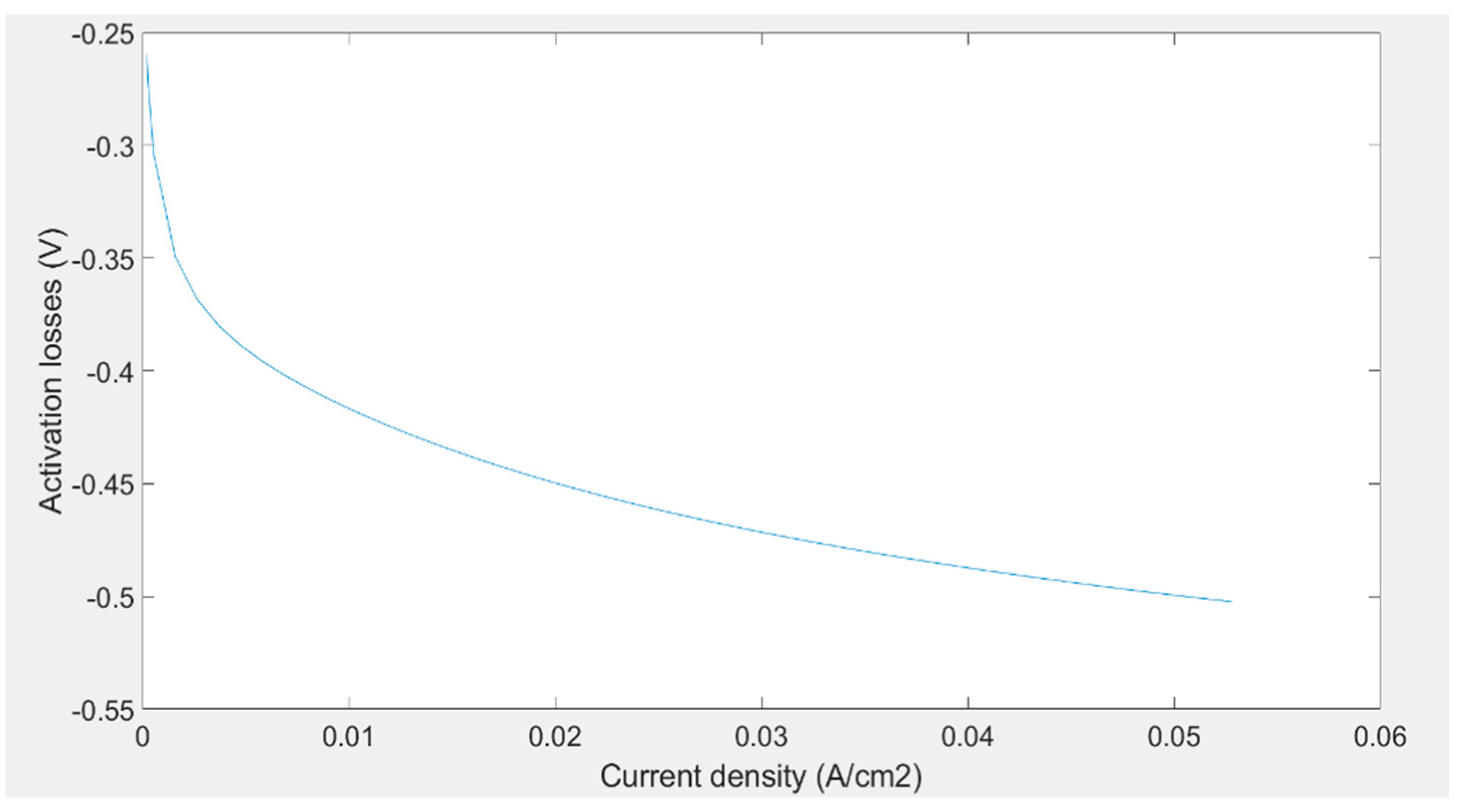
3.1.1. Steady-State Activation Losses

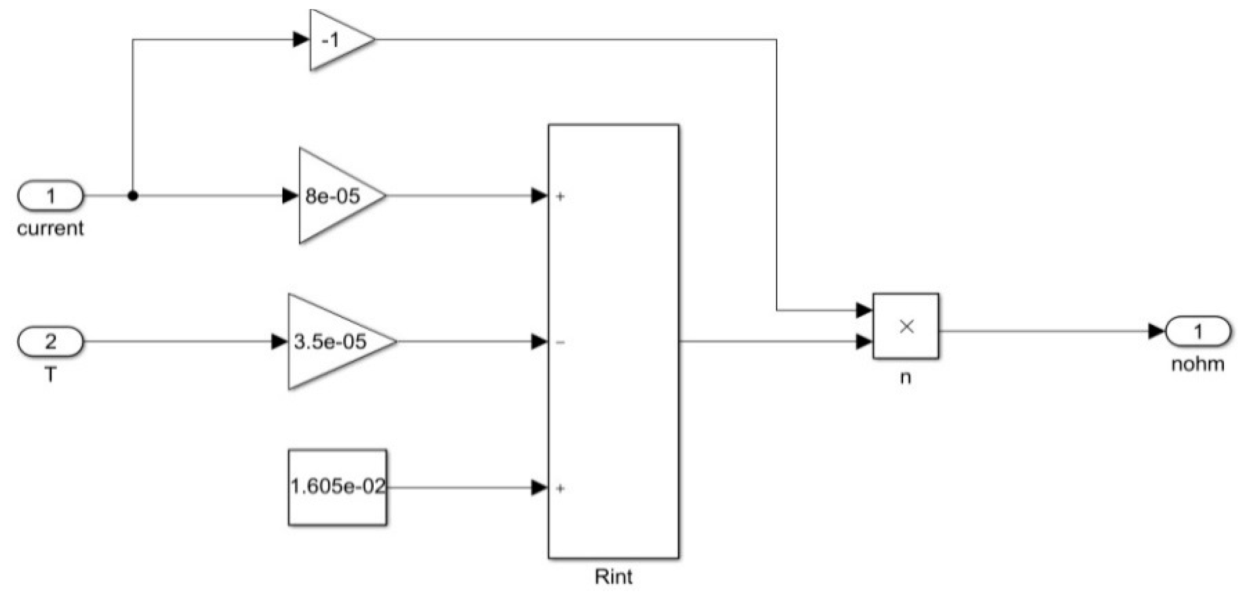
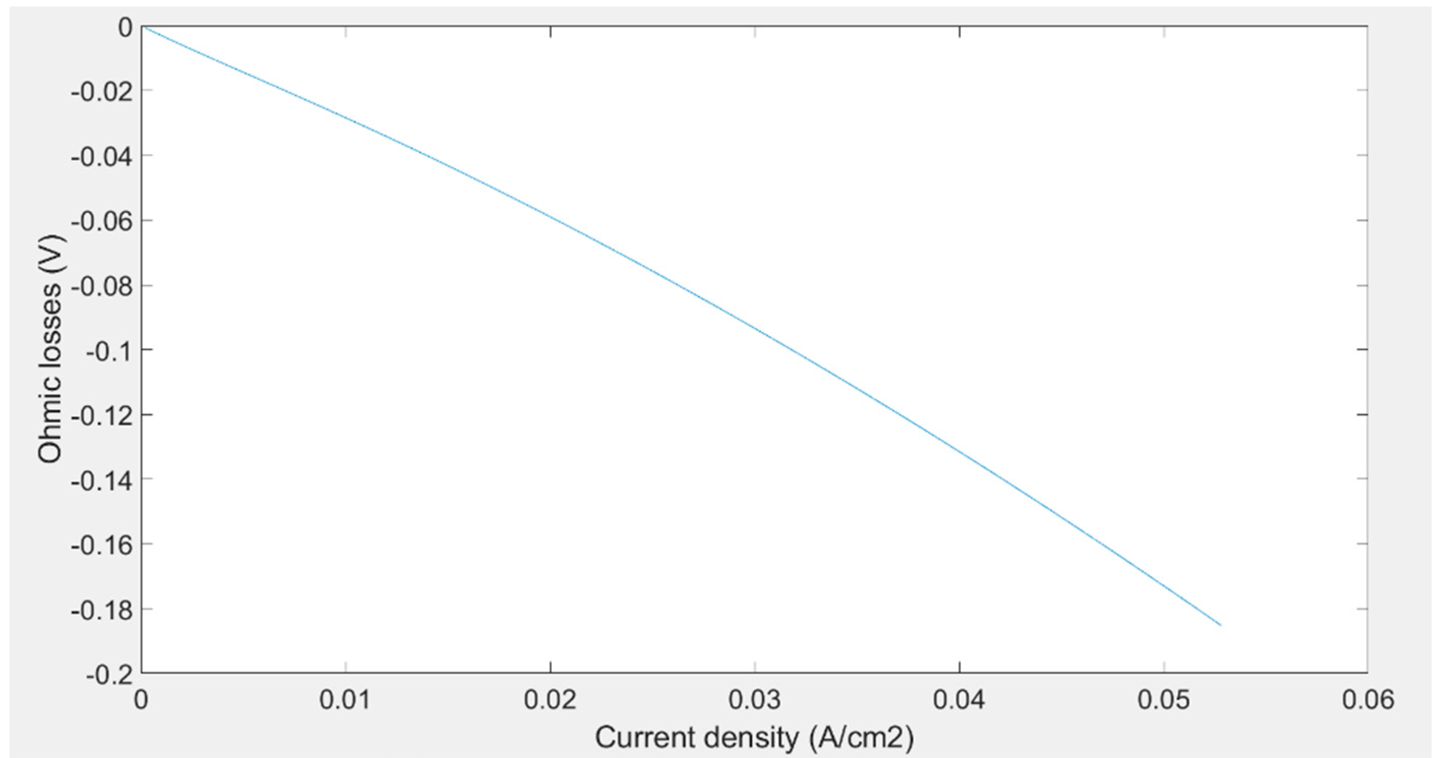
At the first stage, activation losses in a fuel cell arise during the chemical reactions undergoing oxidation and reduction. The losses rise because of the slow rate of reaction at the electrodes. Some fraction of the overall voltage being produced by the fuel cell is used for powering the chemical reaction taking place. Activation losses occur at low current density. They can also be described as the amount of voltage required to start the chemical reaction by overcoming the activation energy required. For low-temperature fuel cells, activation losses are significant and are usually caused by the cathode. As the temperature increases, the activation losses become less significant.

Activation losses are usually represented by the Tafel equations as well as the Butler–Vollmer equation. Both of these equations can be simplified and expanded to derive the following expression:

$$V_{act}={\beta }_1+{\beta }_{2}T+{\beta }_{3}Tln\left(C_{O_2}\right)+{\beta }_{4}Tln\left(i\right)$$

(9)

where β1, β2, β3 and β4 are parametric constants that are dependent upon various constants, taken from [30]. These constants can be substituted in order to simplify the equation. So,

$${\beta }_1= -0.9514$$

(10)

$${\beta }_2= 3.12\ast {10}^{-3}$$

(11)

$${\beta }_3= 7.4\ast {10}^{-5 }$$

(12)

$${\beta }_4= -1.87\ast {10}^{-4}$$

(13)

CO₂ represents the concentration of oxygen. As mentioned earlier, activation losses mainly rise due to the slow rate of reaction occurring at the cathode, i.e., where oxygen combines with protons and electrons in order to produce water. The activation losses at the anode are 0.009 and 0.35 V at the cathode at room temperature of 298 K [30]. It can be deduced that the losses at cathode are more prominent than the losses at anode. The concentration of oxygen can be calculated by:

$$C_{O_2}=\frac{P_{O_2}}{5.08\ast {10}^6\ast e^{\left(-\frac{498}{T_{cell}}\right)}}$$

(14)

3.1.2. Ohmic Losses

During the second stage, as shown in Figure 2, the ohmic losses occur. The linear line in stage 2 depicts these losses. These losses arise due to two resistances that occur in the fuel cell. The first is the resistance that the electrons face when they are flowing through the outer circuit. The second is the resistance that the protons undergo when they are flowing through the proton exchange membrane. These resistances result in the loss of potential of the fuel cell. The total ohmic resistance can therefore be modeled as the sum of electron ohmic losses and the proton ohmic losses. This voltage drop can be explained by simply using Ohm’s law.

$$V_{ohm}=-i\ast R_{int }$$

(15)

where i is the current flowing via the fuel cell and R_int is the overall internal resistance of the fuel cell. The overall internal resistance includes the resistance in wires, bipolar plates, current collector plates, and the proton exchange membrane, etc. R_int can be represented as a function of temperature and current [30]:

$$R_{int}=1.605\ast {10}^{-2}-3.5\ast {10}^{-5}{T}_{cell}+8\ast {10}^{-5}i$$

(16)

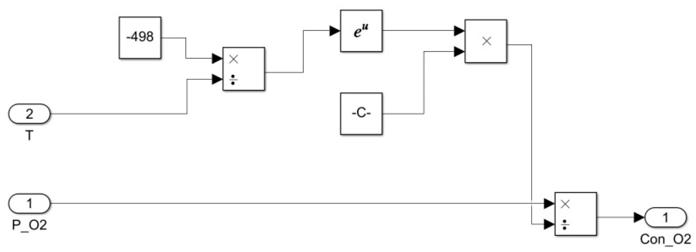
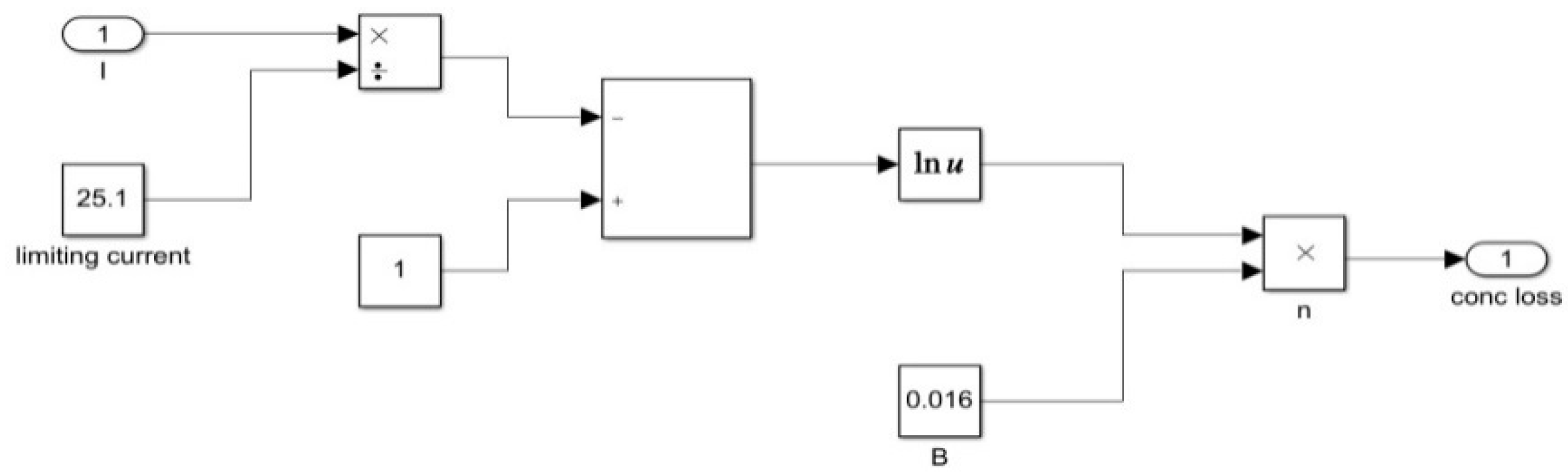
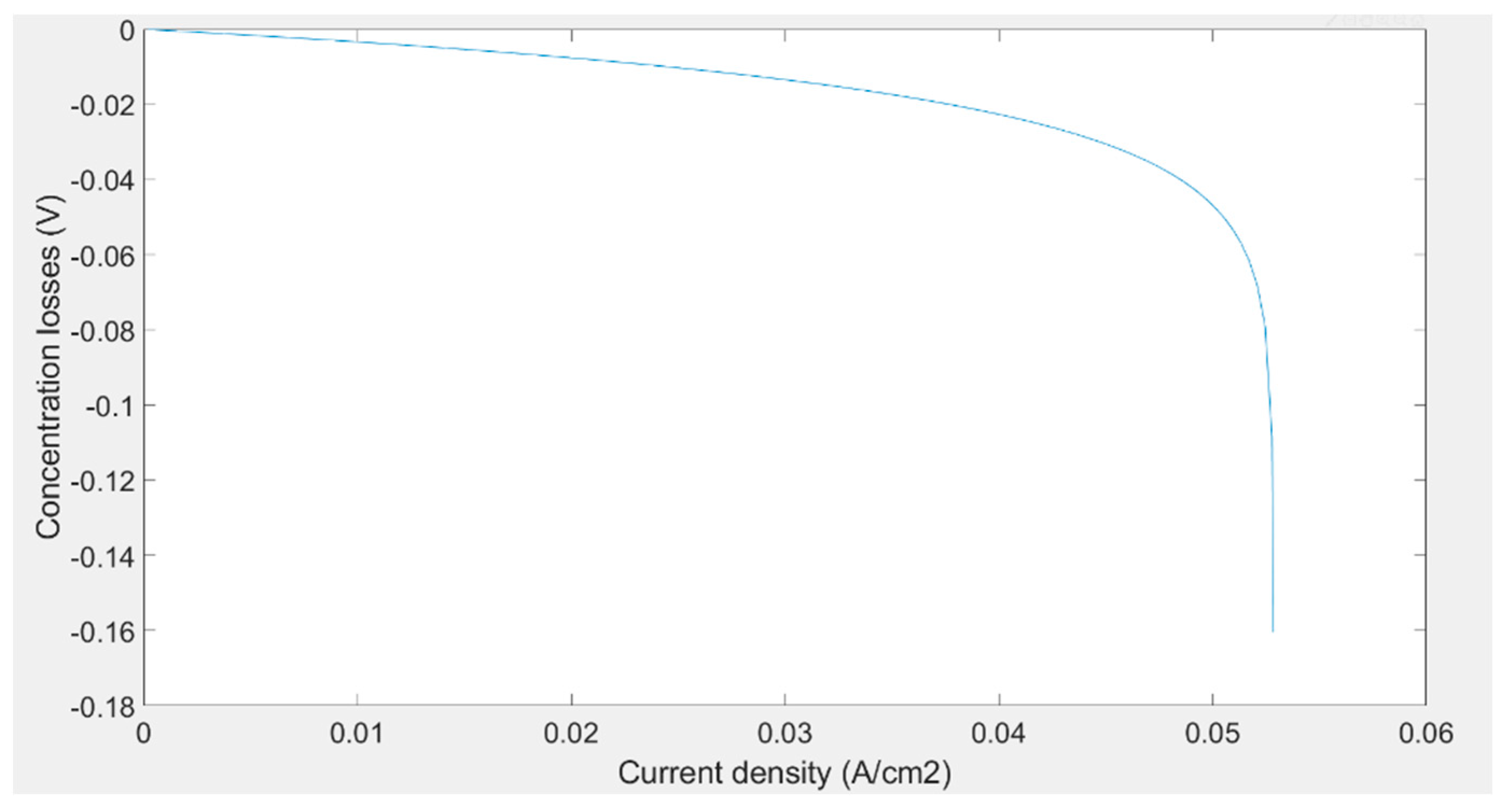
3.1.3. Concentration Losses

During the third and final stage, the concentration losses occur. They are also known as mass transport losses. These losses are related to the concentration of hydrogen and oxygen at the anode and cathode, respectively. At higher current densities, these losses are substantial. As the current density is increased, i.e., further current is drawn from the PEMFC, the amount of fuel and oxygen being consumed increases.

The concentration of the reactants becomes equal to zero when the rate of supply and the rate of consumption of the reactants become equal at the electrode surface. This occurs when the reactants are consumed as soon as they are supplied, and they do not stay on the electrode. The current density at which this phenomenon happens is known as the limiting current density. If the current density is increased beyond this limit, the fuel cell will fail to work, since there will be fewer reactants as the rate of consumption will become greater than the rate of supply [31].

The concentration losses in a fuel cell can be represented by:

$$V_{conc}=B.ln\left(1-\frac{i}{i_{lim}}\right)$$

(17)

where I_lim is the limiting current in the fuel cell. It can be seen from the equation that the value of current cannot be greater than the limiting current, since it will give a non-finite value.

The final output voltage can be calculated by the summation of all the voltage drops and the ideal voltage of the fuel cell.

$$V_{cell}=E-V_{act}-V_{ohm}-V_{conc}$$

(18)

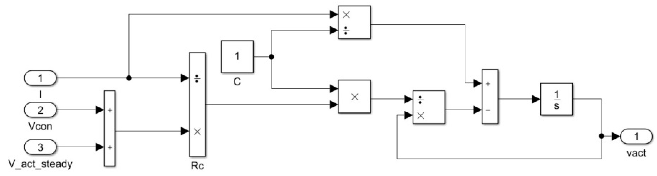
3.2. Dynamic Modeling

The dynamic model of a PEMFC differs from a steady-state model since dynamic activation losses and thermodynamic modeling is also added. A dynamic response of the fuel cell mainly occurs due to the charge double layer (CDL). This effect occurs when two different materials come into contact with one another. This gives rise to the formation and accumulation of a charge on their surface. This charge is then transferred from one material to another. This charge effects the activation and the concentration losses in a fuel cell. In order to predict and analyze the dynamic response, two more equations must be modeled. The first one is the dynamic activation losses, represented by:

$$\frac{d{V}_{act}}{dt}=\frac{i}{C}-\frac{V_{act}}{R_{c}C}$$

(19)

where R_c equals the sum of steady-state activation and concentration losses divided by current, and C represents the double layer charge.

$$R_c=\frac{V_{act,0}+V_{conc}}{i}$$

(20)

The second equation is the thermodynamic response. In a dynamic model, the temperature of a fuel cell does not remain constant, unlike the steady-state model. This temperature is significant since it is used to calculate all other parameters, such as the ideal voltage ‘E’, the three voltage drops, and the partial pressures. The temperature can be determined by

$$C_t\frac{dT}{dt}=i\left(E-V_{cell}\right)-H\left(T_{cell}-T_f\right)$$

(21)

where:

• C_t is the total thermal capacitance;
• H is the total heat transfer coefficient;
• T_f is the reference temperature;
• T_cell is the lumped temperature of the fuel cell.

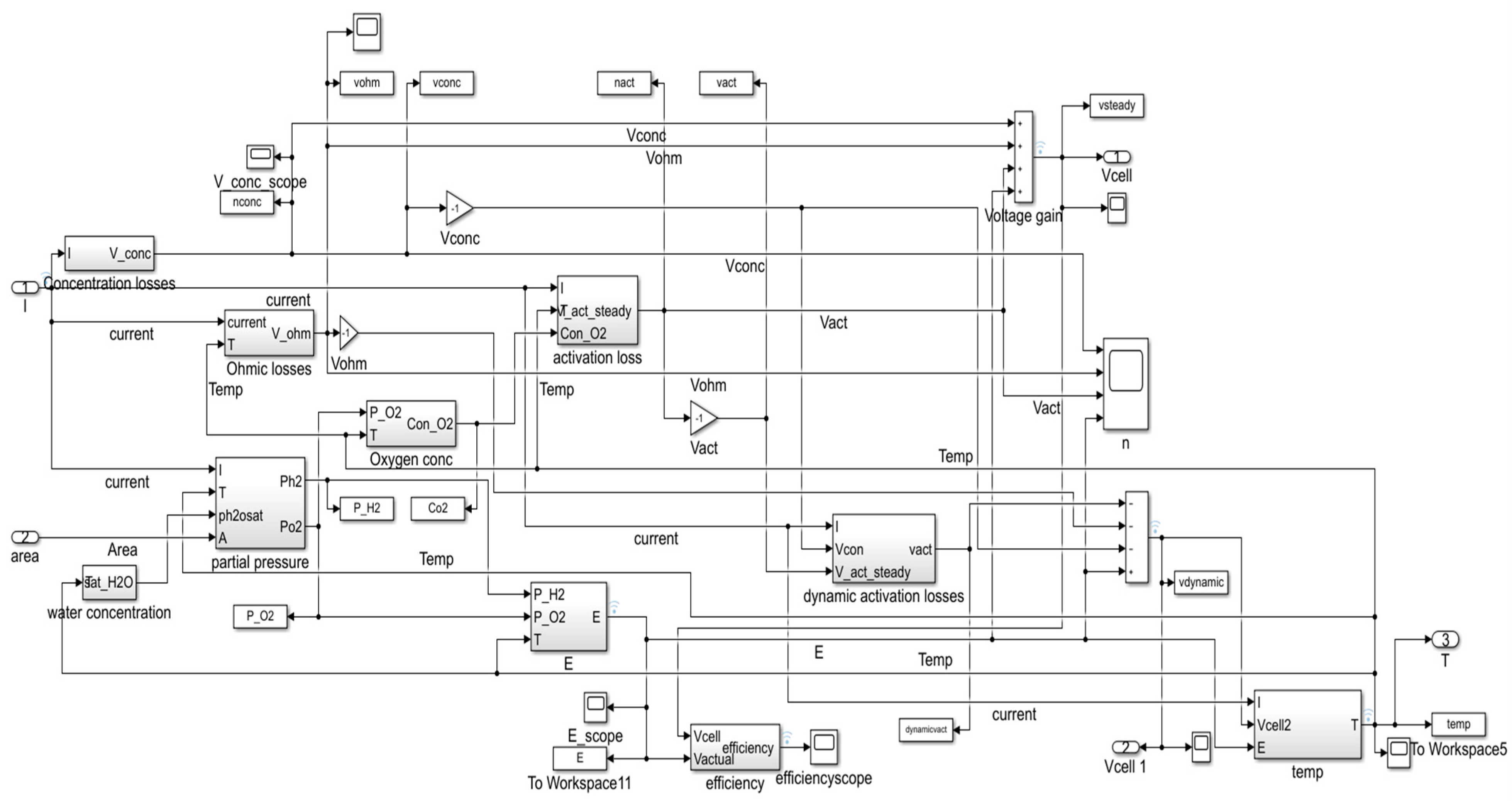
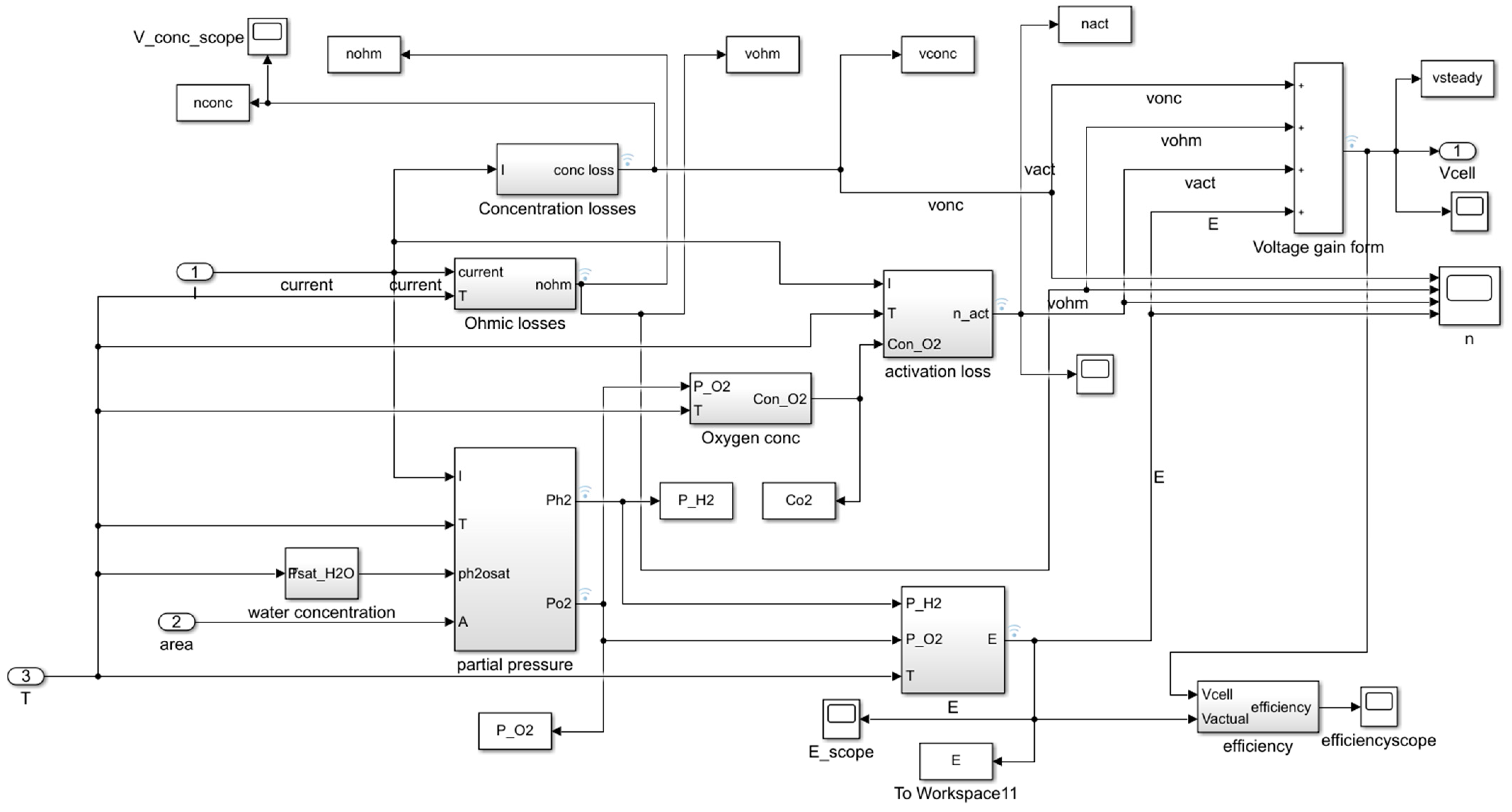
3.2.1. PEMFC Stack Modeling

For both the steady-state and the dynamic model, the values calculated are for a single cell. A fuel cell consists of a number of cells arranged in a manner called a fuel cell stack. The total output voltage can be calculated by taking the product of V_cell and the total number of cells.

$$V_{stack}=n{V}_{cell}$$

(22)

The total power output of the fuel cell stack can be calculated by taking the product of current ‘i’ and the output voltage ‘V_stack’.

3.2.2. Heat Recovery System

As discussed earlier, PEMFCs are not 100% efficient. The remaining percentage of the output that is not converted into power is converted into heat. This heat can be recovered with the help of a cooling fluid. For this paper, the heat is recovered by using the working fluid of the ORC. The recovered heat can then be used to run a separate system. For this paper, the recovered heat will be used to run an organic Rankine cycle (ORC).

3.3. Thermodynamic Analysis of the Cycle

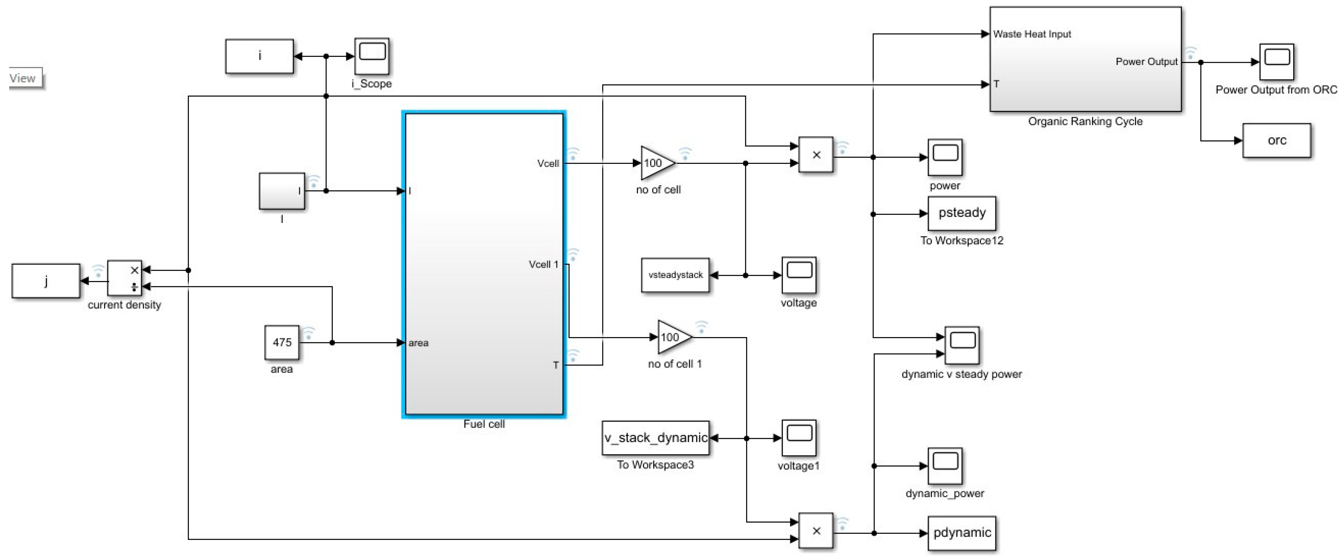
A thermodynamic cycle is analyzed by using certain formulas that require a number of thermodynamic properties. The values of enthalpy, density, etc., were determined using COOLPROP and were later verified by using REFPROP version 8.0 [32]. In order to determine these properties at a certain point in the cycle, two properties at that particular point must be known. These properties can vary from temperature and pressure to the vapor quality. The Temperature-Entropy (T–S) diagram of the ORC is illustrated in Figure 4.

The pump is a work consuming device that undergoes no heat transfer. The pump is assumed to work isentropically. The enthalpy at point 1, h₁, in the cycle can be determined by taking the pressure of the condenser and a vapor quality of 0 (since the fluid is a saturated liquid at this point). The value of entropy s₁ is also determined at this point in order to determine the value of h₂ at point 2. This point is the pump exit. Hence h₂ is determined by using s₁ and evaporator pressure. The work consumed in a pump, per unit mass, can be determined by

$$w_{pump,in}=h_2-h_{1 }$$

(23)

The pump work can also be calculated by using the specific volume at that point and the pressure difference between the evaporator and the condenser.

$$w_{pump,in}=v(P_2-P_1)$$

(24)

where the specific volume is calculated by using density, ρ, at point 1.

$$v=\frac{1}{\rho }$$

(25)

The evaporator does not involve any work but does undergo a heat transfer process. The evaporator exchanges heat with the heat source in order to vaporize the zeotropic mixture. The amount of heat input to the system per unit mass basis is calculated by

$$q_{in}=h_3-h_2$$

(26)

where h₃ and h₂ indicate the enthalpies at the evaporator outlet and inlet, respectively.

The turbine undergoes rotation in order to produce work by the expansion of the superheated vapor. It is a work-producing device. This work output is utilized for the operation of the pump and the generator for the production of electricity. The turbine work output is calculated by

$$w_{turb,out}=h_3-h_4$$

(27)

The condenser carries out the exchange of heat with the sink and hence it involves a heat transfer process without any work. The condenser rejects heat, which can be calculated by

$$q_{out}=h_4-h_1$$

(28)

The net work output of the overall cycle is given by the work produced by the turbine and the work consumed by the pump. It can also be represented by the net difference of heat input and heat output of the system.

$$w_{net}=w_{turb,out}-w_{pump,in}=q_{in}-q_{out}$$

(29)

The overall thermal efficiency of the cycle is given by

$${\eta }_{th}=\frac{w_{net}}{q_{in}}=1-\frac{q_{out}}{q_{in}}$$

(30)

3.4. Simulink Model

The following models were created using Simulink R2016a. Figure 5 shows the ideal voltage, i.e., E Nernst voltage.

Figure 6, Figure 7 and Figure 8 shows the partial pressures, water saturation pressure, and the concentration of oxygen, respectively.

Figure 9, Figure 10 and Figure 11 shows the three losses, i.e., steady-state activation, concentration, and ohmic losses, respectively.

Figure 12 shows the dynamic activation voltage.

Figure 13 shows the dynamic temperature model.

Figure 14 and Figure 15 show the fuel stack model and the ORC model, respectively.

Figure 16 and Figure 17 show the parent assembly for a dynamic and steady-state model, respectively. The parent assembly is the main assembly under which all the subsystems are performing.

4. Discussion

The modeling of the fuel cell was done on MATLAB/ Simulink R2016a. The models created for the simulation were all based on the equations given in this paper. The parameters of the fuel cell are based on the Horizon H-500 fuel cell, as described in

Table 1. Horizon H-500 parameters.

Parameter	Value
No. of cells	100
Area of the cell	475 cm2
Rated current performance	24 A
External temperature	303.15 K
Pressure at anode	1.45 atm
Pressure at cathode	1 atm
Concentration loss coefficient	0.016
Limiting current	25.1 A
Total thermal capacitance	10 J/K
Total heat transfer coefficient	10 W/K
Maximum stack temperature	63 °C

[33].

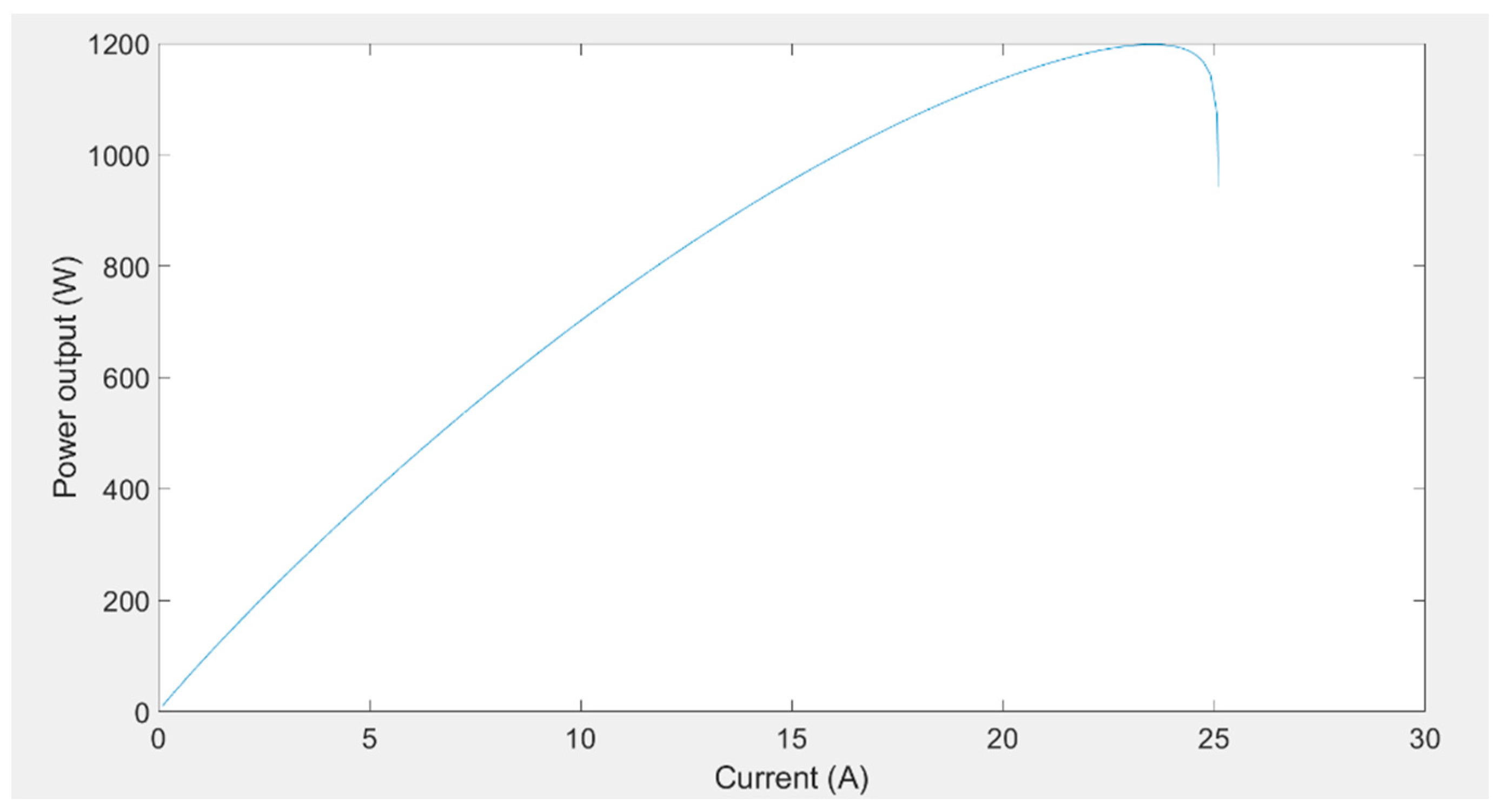
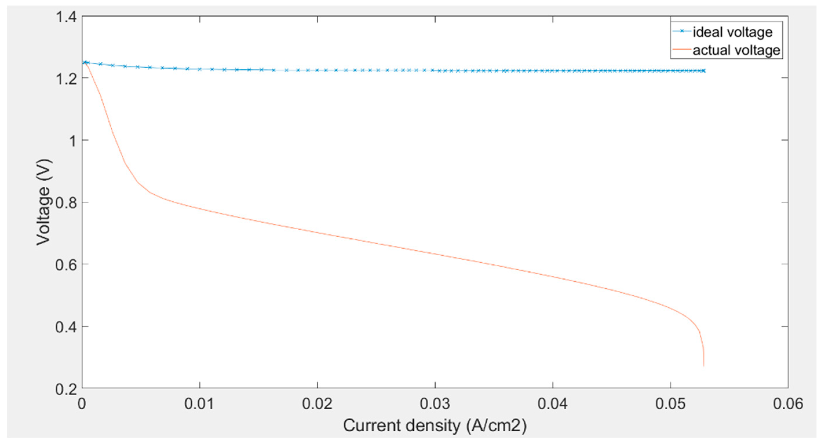
4.1. Performance of a Single PEMFC Cell

Figure 18 shows the polarization curve of the PEMFC under the given parameters. The curve starts at the maximum value, i.e., the ideal voltage. The three potential losses cause the voltage to drop. At low current densities, the activation losses dominate and the graph decreases. The linear portion in the middle represents the losses due to the ohmic losses. The significant drop in the end shows the concentration losses. It can be noticed from the polarization curve that the overall voltage of the fuel cell decreases with increasing current density.

Figure 19 shows the ideal cell voltage. The graph shows a straight line, i.e., a constant output voltage that remains constant, regardless of the current density. If the cell were to operate under conditions where no losses occur, then this graph will be achieved.

Figure 20 shows the steady-state activation losses against current density. It can be noticed that at lower current density, the activation losses dominate, and a steep drop can be noticed in the beginning. This is because of the slow start of the reaction. Additionally, the initial voltage output is used to overcome the activation energy of the reaction. Furthermore, the reaction at the cathode, i.e., the reduction of oxygen and formation of water, is a slow process, and this is why the activation losses depend on the concentration of oxygen.

Figure 21 shows the graph of ohmic losses against current density. The graph of ohmic losses is linear. As the reaction proceeds and the current density increases, the resistance being offered by the fuel cell components increases. This is mainly due to the resistances of the wire, the bipolar plate, and the proton exchange membrane, etc.

Figure 22 shows the concentration losses that occur towards the end of the polarization curve. It can be observed that these losses rise as current density increases. They drop drastically at a point where the limiting current occurs. At this point, the concentration of reactants at the electrode become equal to zero. As the current being drawn from the fuel cell increases above the limiting current, the reactants being consumed become greater than the reactant being supplied. The fuel cell stops working when this occurs, hence the steep drop in the voltage.

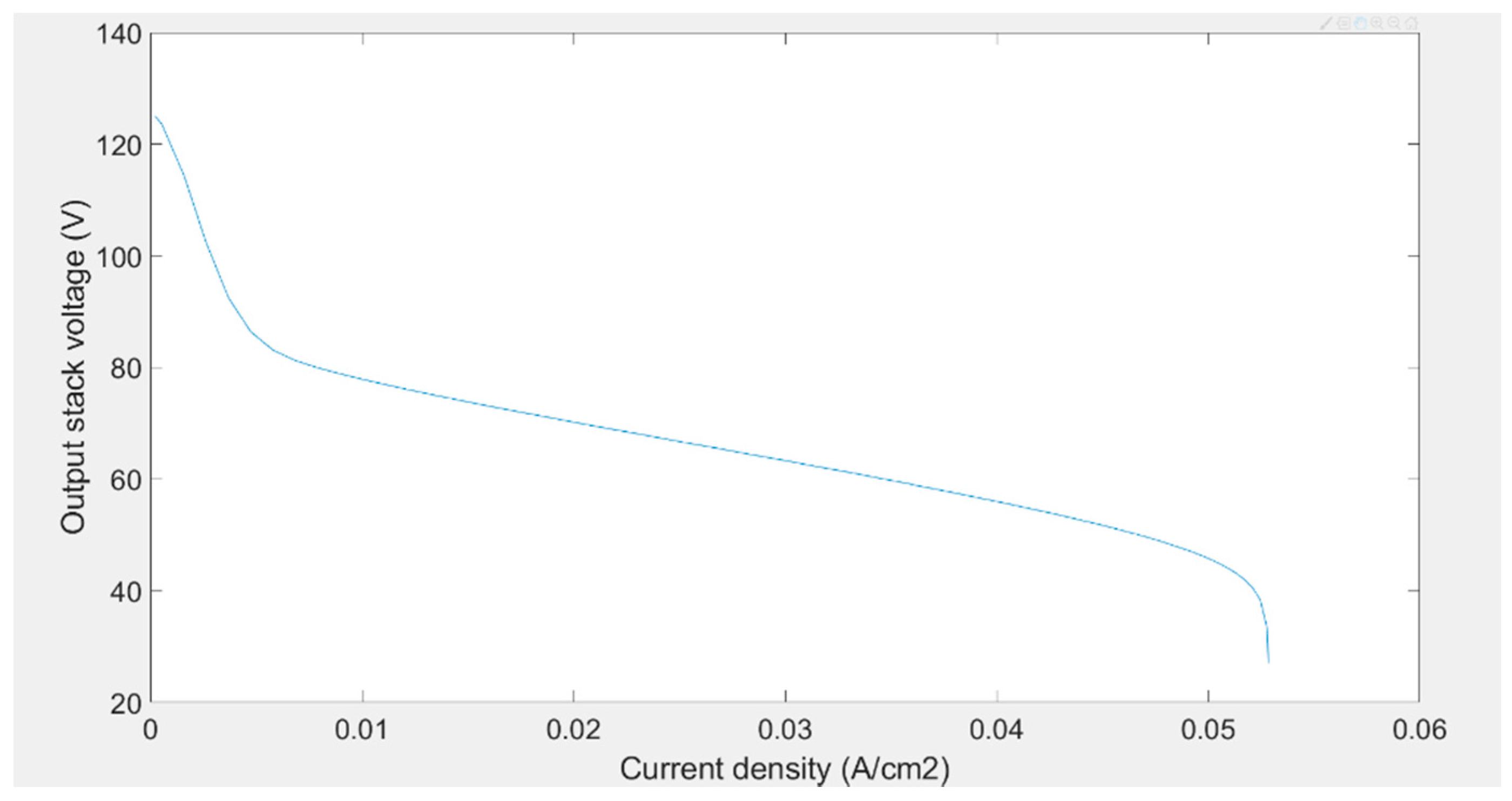
4.2. Performance of PEMFC Stack

Figure 23 shows the steady power output of the PEMFC. The power is obtained by taking the product of the input current and the output voltage. Stack power output shows an increasing trend up to a specific value. At this value of rated current, the maximum power output occurs. Increasing the current beyond this point results in a fall in power output. This is because the value of the current approaches the limiting current and starts to decrease as concentration losses dominate. The maximum power of 1198 W is achieved at the current of around 24 A, after which the power starts to fall.

Figure 24 shows the comparison between the graphs of steady-state power and dynamic power. For the dynamic model, the thermodynamic subsystem was modeled, and the output value of temperature was input into the system. For the steady-state model, a constant temperature value of 336 K was obtained. For the steady-state system, the power output is 1198 W, while for the dynamic system, the power output is 1110 W. There is difference of 7.35% between the two. The dynamic power output is lower due to the dynamic activation losses and the temperature differences.

Figure 25 shows how the ideal cell voltage varies with the actual cell voltage. Ideally, the output voltage should be constant, but due to losses in the fuel cell during the three stages, the voltage drops.

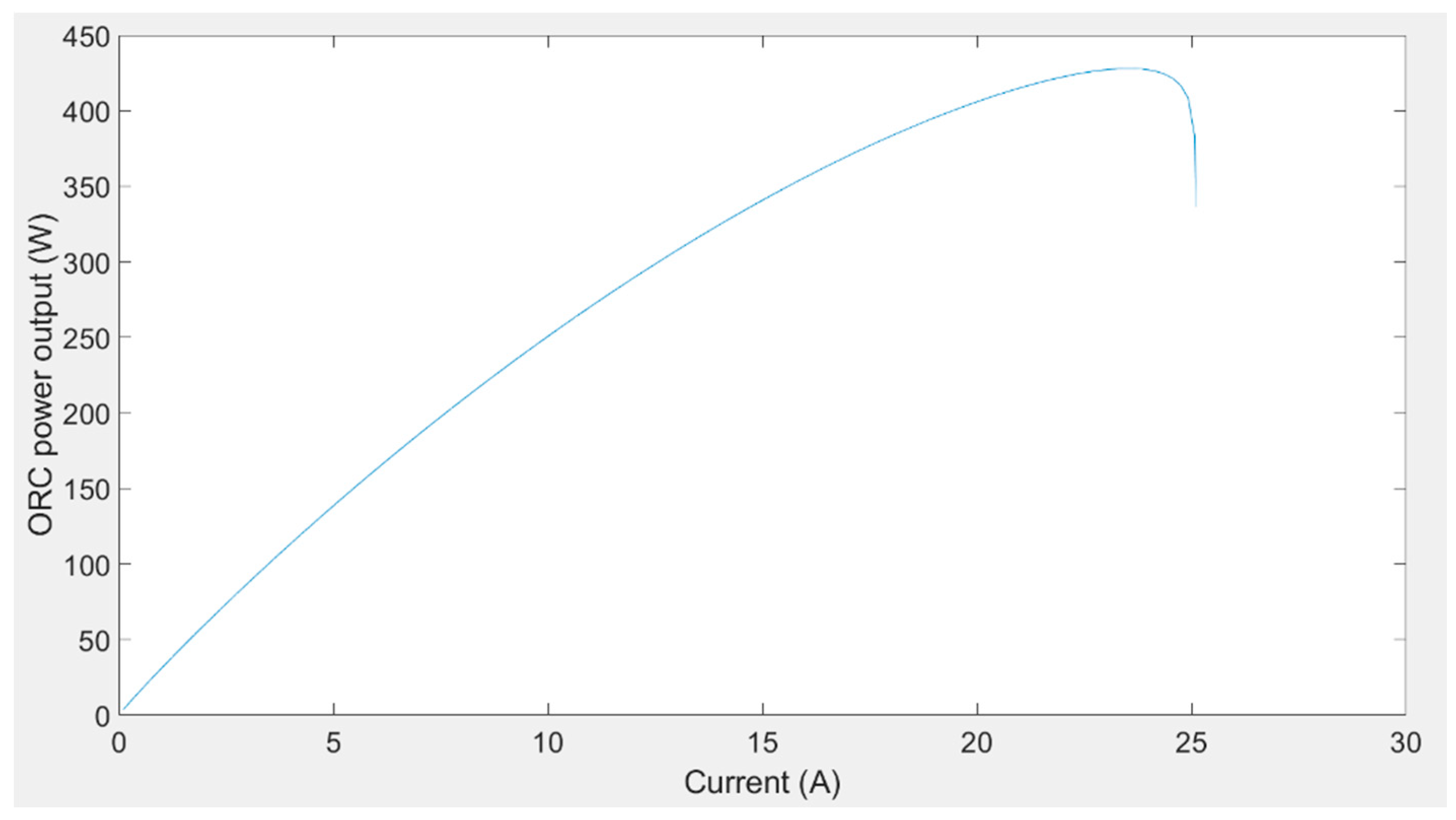
4.3. ORC Working on Recovered Heat

Since the efficiency of the PEMFC is taken as 50%, the amount of power produced is equal to the amount of heat generated. Hence, the power output can be taken as the heat input into the ORC system. For this system, the steady output power is taken. So, the heat input is 1198 W. The zeotropic mixture used in the ORC is also used as a coolant for the fuel cell. The mixture extracts heat from the fuel cell and vaporizes in what can be modeled as the evaporator. The zeotropic mixture used is R-404a. The maximum power produced by the ORC is 428 W. Hence the overall power output of the combined system is 1626 W for a steady-state condition. The power output from the system is shown in Figure 26.

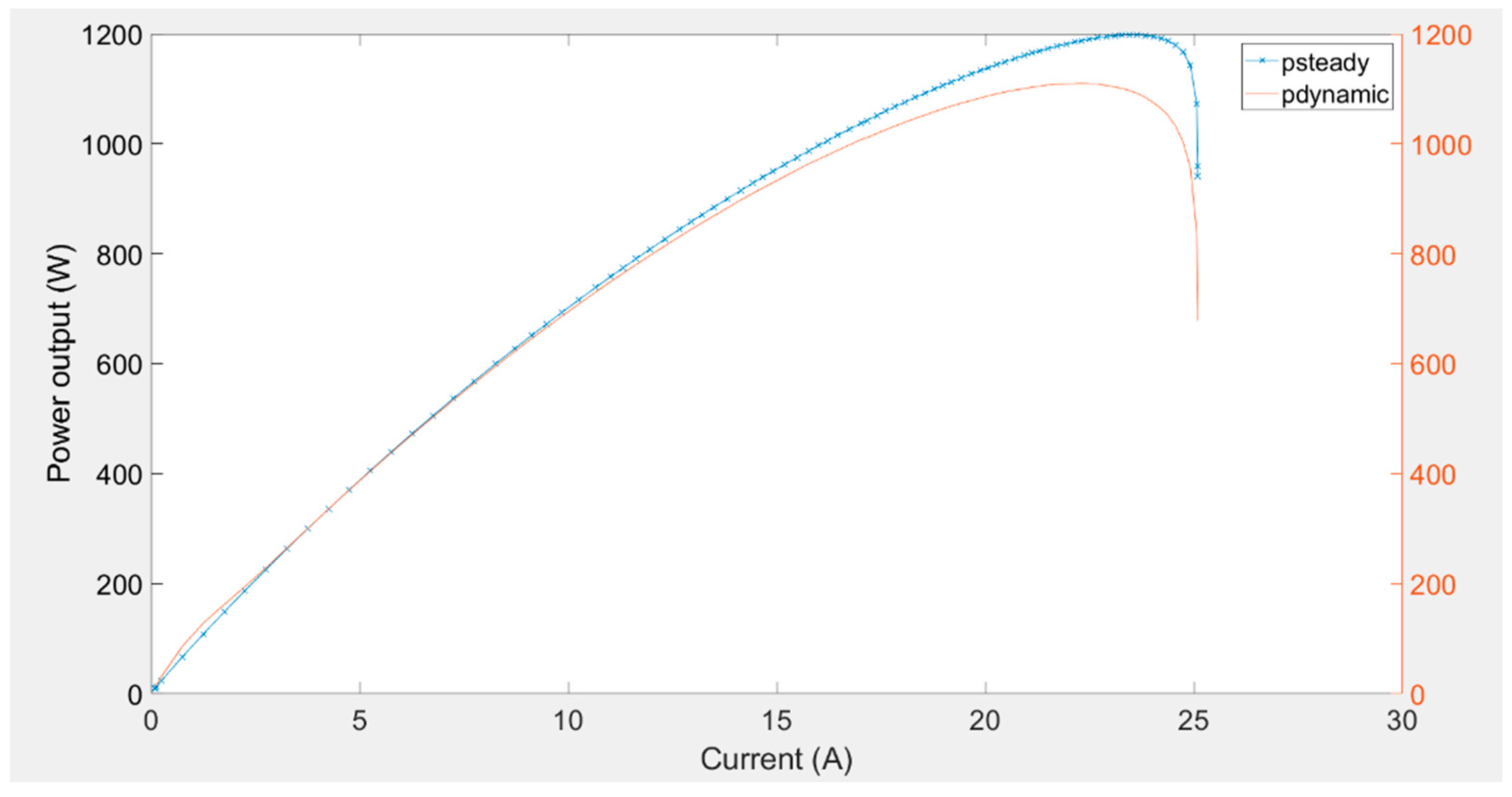
4.4. Model Verification

The model is verified against the given paper [13]. The model given by Azri et al. operates on similar parameters. By setting the parameters for this simulation similar to those given in the reference, the values can be compared to validate the model. For this comparison, a stacking of 36 cells is used.

Table 2. Model comparison.

Parameter	Simulation	Azri et al.	% Age Difference
Power output (W)	410	435	6.1%
Rated current density (A)	0.052	0.053	1.92%
Stack voltage (V)	45	45	0%

compares the values of this simulation against the one given in [13] and shows the percentage difference between the simulation and the reference paper.

5. Conclusions

This paper discusses the steady-state and dynamic models of a proton exchange membrane fuel cell developed on Simulink. It was concluded that the highest power that the fuel cell can produce was 1198 W at a current of 24 A under steady-state conditions. These values are for the Horizon H-500 fuel cell with fixed input parameters. These values give us an idea of how the system will perform under actual conditions and at what parameters the maximum power can be achieved. By running a simulation, the performance of the fuel cell can be analyzed before fabrication, which reduces the chances of failure and defects. The model in this paper is applicable for both steady-state and dynamic systems. Since the parameters can be varied easily, this model can be used with a wide range of fuel cells.

The ORC system given in this paper produces a power output of 428 W with a given waste heat input of 1198 W from the fuel cell. This gives the system an efficiency of around 35%. The output voltage follows the typical behavior of a PEMFC voltage curve. It decreases as the current rises due to various losses, as discussed in the paper. However, the limitations of proposed study are the issues that are related to storage and transport of hydrogen for PEMFC and the high cost of PEMFC that results in an overall increase in the system cost. Moreover, use of ORC in the proposed study produces less power as compared to the steam cycle. In addition, the fluid used in ORC is a combustible fluid— therefore, issues related to fuel combustibility do exist. Additionally, many of the practical considerations of an ORC (physical integration with current system, cost, etc.) remain to be explored. Solutions to these issues will be proposed in future studies.

References

1. Renewables 2019 Global Status Report; Renewable Energy Policy Network for the 21st Century; REN21: Paris, France, 2019.
2. Larminie, J.; Dicks, A. Fuel Cell Systems Explained, 2nd ed.; John Willey & Sons Ltd.: Hoboken, NJ, USA, 2003. [Google Scholar]
3. Ioannou, S.G. Discrete Linear Constrained Multivariate Optimization for Power Sources of Mobile Systems; University of South Florida: Tampa, FL, USA, 2008. [Google Scholar]
4. Ioannou, S.; Dalamagkidis, K.; Valavanis, K.P.; Stefanakos, E.K.; Wiley, P.H. On Improving Endurance of Unmanned Ground Vehicles: The ATRV-Jr Case Study. In Proceedings of the 2006 14th Mediterranean Conference on Control and Automation, Ancona, Italy, 28–30 June 2006; pp. 1–6. [Google Scholar]
5. Mekhilef, S.; Saidur, R.; Safari, A. Comparative study of different fuel cell technologies. Renew. Sustain. Energy Rev. 2012, 16, 981–989. [Google Scholar] [CrossRef]
6. Kreutz, T.G.; Ogden, J.M. Assessment of Hydrogen-Fueled Proton Exchange Membrane Fuel Cells for Distributed Generation and Cogeneration. In Proceedings of the 2000 U.S. DOE Hydrogen Program Review, San Ramon, CA, USA, 9–11 May 2000. [Google Scholar]
7. Ural, Z.; Gençoğlu, M.T.; Gümüs, B. Dynamic Simulation of a Pem Fuel Cell System. In Proceedings of the 2nd International Hydrogen Energy Congress and Exhibition IHEC 2007, Istanbul, Turkey, 13–15 July 2007. [Google Scholar]
8. Mammar, K.; Chaker, A. Neural NetworkBased Modeling of PEM fuel cell and Controller Synthesis of a stand-alone system for residential. Int. J. Comput. Sci. 2012, 9, 13–15. [Google Scholar]
9. Yu, X.; Starke, M.; Tolbert, L.; Ozpineci, B. Fuel cell power conditioning for electric power applications: A summary. IET Electr. Power Appl. 2007, 1, 643. [Google Scholar] [CrossRef]
10. Wang, Y.; Chen, K.S.; Mishler, J.; Cho, S.C.; Adroher, X.C. A review of polymer electrolyte membrane fuel cells: Technology, applications, and needs on fundamental research. Appl. Energy 2011, 88, 981–1007. [Google Scholar] [CrossRef] [Green Version]
11. Francesconi, J.A.; Mussati, M.C.; Aguirre, P.A. Effects of PEMFC operating parameters on the performance of an integrated ethanol processor. Int. J. Hydrogen Energy 2010, 35, 5940–5946. [Google Scholar] [CrossRef]
12. Li, Q.; Jensen, J.O.; Savinell, R.F.; Bjerrum, N.J. High temperature proton exchange membranes based on polybenzimidazoles for fuel cells. Prog. Polym. Sci. 2009, 34, 449–477. [Google Scholar] [CrossRef] [Green Version]
13. Azri, M.; Mubin, A.N.A.; Ibrahim, Z.; Rahim, N.A.; Raihan, S.R.S. Mathematical Modelling for Proton Exchange Membrane Fuel Cell (PEMFC). J. Theor. Appl. Inf. Technol. 2016, 86, 409–419. [Google Scholar]
14. Benchouia, N.; Hadjadj, A.E.; Derghal, A.; Khochemane, L.; Mahmah, B. Modeling and validation of fuel cell PEMFC. Rev. Energ. Renouv. 2013, 16, 365–377. [Google Scholar]
15. Macedo-Valencia, J.; Sierra, J.; Figueroa-Ramírez, S.; Mandujano, H.; Meza, M.; Tadeo, J.; Grajeda, S. Numerical study of heat transfer in a PEM fuel cell with different flow-fields. In Proceedings of the XV International Congress of the Mexican Hydrogen Society, Mexico City, Mexico, 22–25 September 2015. [Google Scholar]
16. Santarelli, M.; Torchio, M.F.; Cochis, P. Parameters estimation of a PEM fuel cell polarization curve and analysis of their behavior with temperature. J. Power Sources 2006, 159, 824–835. [Google Scholar] [CrossRef]
17. Xue, X.; Cheng, K.W.E.; Sutanto, D. Unified mathematical modelling of steady-state and dynamic voltage-current characteristics for PEM fuel cells. Electrochim. Acta 2006, 52, 1135–1144. [Google Scholar] [CrossRef]
18. Zhao, J.; Jian, Q.; Luo, L.; Huang, B.; Cao, S.; Huang, Z. Dynamic behavior study on voltage and temperature of proton exchange membrane fuel cells. Appl. Therm. Eng. 2018, 145, 343–351. [Google Scholar] [CrossRef]
19. WLin; Yuan, J.; Sundén, B. Waste Heat Recovery for Fuel Cell System. In Proceedings of the International Green Energy Conference, Waterloo, ON, Canada, 1–3 June 2010. [Google Scholar]
20. Cao, Y. Analysis of an energy recovery system for reformate-based PEM fuel cells involving a binary two-phase mixture. J. Power Sources 2005, 141, 258–264. [Google Scholar] [CrossRef]
21. Venkataraman, V.; Pacek, A.W.; Steinberger-Wilckens, R. Coupling of a Solid Oxide Fuel Cell Auxiliary Power Unit with a Vapour Absorption Refrigeration System for Refrigerated Truck Application. Fuel Cells 2016, 16, 273–293. [Google Scholar] [CrossRef]
22. Fuchs, M. Study of High Temperature Pem Fuel Cell (HT-PEMFC) Waste Heat Recovery through Ejector Based Refrigeration. Ph.D. Thesis, Florida Atlantic University, Boca Raton, FL, USA, 2012. [Google Scholar]
23. Guo, X.; Zhang, H.; Zhao, J.; Wang, F.; Wang, J.; Miao, H.; Yuan, J. Performance evaluation of an integrated high-temperature proton exchange membrane fuel cell and absorption cycle system for power and heating/cooling cogeneration. Energy Convers. Manag. 2019, 181, 292–301. [Google Scholar] [CrossRef]
24. Sharaf, O.Z.; Orhan, M.F. An overview of fuel cell technology: Fundamentals and applications. Renew. Sustain. Energy Rev. 2014, 32, 810–853. [Google Scholar] [CrossRef]
25. Liu, G.; Qin, Y.; Wang, J.; Liu, C.; Yin, Y.; Zhao, J.; Yin, Y.; Zhang, J.; Otoo, O.N. Thermodynamic modeling and analysis of a novel PEMFC-ORC combined power system. Energy Convers. Manag. 2020, 217, 112998. [Google Scholar] [CrossRef]
26. Chowdhury, J.I. Modelling of Evaporator in Waste Heat Recovery System using Finite Volume Method and Fuzzy Technique. Energies 2015, 8, 14078–14097. [Google Scholar] [CrossRef] [Green Version]
27. Lemmon, E.; Huber, M.; McLinden, M. NIST Standard Reference Database 23e Version 8.0, Physical and Chemical Properties Division; National Institute of Standards and Technology/US Department of Commerce: Boulder, CO, USA, 2002. [Google Scholar]
28. Huang, X. Fuel Cell Technology for Distributed Generation: An Overview. In Proceedings of the 2006 IEEE International Symposium on Industrial Electronics, Montreal, QC, Canada, 9–13 July 2006. [Google Scholar]
29. Electrocatalyst Degradation in High Temperature PEM Fuel Cells, ANNO ACCADEMICO 2013/2014. Available online: https://www.openstarts.units.it/bitstream/10077/11126/1/PhD%20Thesis%20-%20F.%20Valle.pdf (accessed on 5 November 2020).
30. Mahapatra, M.K.; Singh, P. Fuel Cells: Energy Conversion Technology. In Future Energy; Elsevier: Amsterdam, The Netherlands; pp. 511–547.
31. Amphlett, J.C.; Baumert, R.M.; Mann, R.F.; Peppley, B.A.; Roberge, P.R.; Harris, T.J. Performance modeling of the Ballard Mark IV solid polymer electrolyte fuel cell: I. Mechanistic model development. J. Electrochem. Soc. 1995, 142, 1. [Google Scholar] [CrossRef]
32. Barbir, F. PEM fuel cells. In Fuel Cell Technology; Springer: London, UK, 2006; pp. 27–51. [Google Scholar]
33. Horizon Fuel Cell Technologies. 2013. Available online: http://www.horizonfuelcell.com/ (accessed on 5 November 2020).
Figure 1. Components of an organic Rankine cycle (ORC) [26].
Sustainability 13 01218 g001
Figure 2. Polarization curve of a proton exchange membrane fuel cell (PEMFC) [28].
Sustainability 13 01218 g002
Figure 3. Three stages of voltage drop [29].
Sustainability 13 01218 g003
Figure 4. T–S diagram of an ORC.
Sustainability 13 01218 g004
Figure 5. E Nernst simulation model.
Sustainability 13 01218 g005
Figure 6. Partial pressures of hydrogen and oxygen.
Sustainability 13 01218 g006
Figure 7. Saturation pressure of H2O.
Sustainability 13 01218 g007
Figure 8. Oxygen concentration block diagram.
Sustainability 13 01218 g008
Figure 9. Steady state activation losses.
Sustainability 13 01218 g009
Figure 10. Concentration losses.
Sustainability 13 01218 g010
Figure 11. Ohmic losses.
Sustainability 13 01218 g011
Figure 12. Dynamic activation losses.
Sustainability 13 01218 g012
Figure 13. Thermodynamic model.
Sustainability 13 01218 g013
Figure 14. Fuel stack block diagram.
Sustainability 13 01218 g014
Figure 15. ORC block diagram.
Sustainability 13 01218 g015
Figure 16. Dynamic model parent assembly.
Sustainability 13 01218 g016
Figure 17. Steady state parent assembly.
Sustainability 13 01218 g017
Figure 18. Polarization curve of Horizon H-500 fuel cell.
Sustainability 13 01218 g018
Figure 19. Ideal cell voltage.
Sustainability 13 01218 g019
Figure 20. Steady-state activation losses.
Sustainability 13 01218 g020
Figure 21. Ohmic losses.
Sustainability 13 01218 g021
Figure 22. Concentration losses.
Sustainability 13 01218 g022
Figure 23. Steady-state power output.
Sustainability 13 01218 g023
Figure 24. Steady-state vs. dynamic power output.
Sustainability 13 01218 g024
Figure 25. Ideal voltage vs. actual voltage.
Sustainability 13 01218 g025
Figure 26. ORC power output.
Sustainability 13 01218 g026