
MRP-PCI: A Multiple Reference Point Based Partially Compensatory Composite Indicator for Sustainability Assessment


Department of Applied Economics (Mathematics), University of Málaga, Calle Ejido, 6, 29071 Málaga, Spain
*
Author to whom correspondence should be addressed.
Sustainability 2021, 13(3), 1261; https://0-doi-org.brum.beds.ac.uk/10.3390/su13031261
Submission received: 14 December 2020
/
Revised: 19 January 2021
/
Accepted: 21 January 2021
/
Published: 26 January 2021
(This article belongs to the Special Issue Multiple Criteria Decision Making for Sustainable Development)
Abstract
:Assessing different types of sustainability is a complex procedure, which implies considering aspects of very different nature. One way to do this is using a system of single indicators measuring all these different aspects and aggregating them in an overall composite indicator. In line with the concepts of weak and strong sustainability, the compensability degree among the indicators allowed by the aggregation procedure is a crucial issue. There exist methods that allow for full compensability, zero compensability, or partial compensability. In most of them, the compensation degree is established in a global way, that is, it is the same for all the indicators. In this paper, we develop the Multiple Reference Point Partially Compensatory Indicator (MRP-PCI), where a different compensation index can be established for each indicator. The resulting method can be applied to any system of indicators, and successfully considers the compensation indices given. Some examples and comparisons are used to illustrate its behavior.
1. Introduction
The different types of sustainability are frequently assessed by considering a set (system) of indicators (see, e.g., [1,2]). Nevertheless, there are usually a great number of indicators available, which make it difficult to have an idea of the overall performance of a territory. For this reason, it is usual to synthesize the information provided by the different single indicators into a composite measure, usually known as a composite indicator. Many schemes have been suggested for building composite indicators all of which have three main stages (not necessarily in the same order):
- Normalization. In most of the cases, the individual indicators are measured in different scales and therefore, it is necessary to bring them all down to a common scale before building the composite indicator.
- Weighting. We believe that the construction of composite indicators is essentially subjective. The weights indicate the contribution that, according to the decision center, each single indicator should make to the composite measure. In this sense, it is important to point out that even methods regarded as fully objective (for example, some purely statistical schemes) do imply more or less hidden assumptions about the weights of the indicators, which can be as arguable as other more explicit schemes.
- Aggregation. Finally, once normalized and weighted, the individual indicators are aggregated to get the final composite indicator.
Although all these three stages are equally important, this paper deals basically with the aggregation stage (although the methogology proposed incorporates a specific normalization procedure as well). In most of the published literature addressing the construction of composite indicators, an issue is regarded as critical in this aggregation phase: the compensability issue [3]. That is, when aggregating several single indicators, can a bad performance in one of them be compensated by a good performance in another one, or not? This issue is very important because it critically affects the value of the composite indicator. If a fully compensatory scheme is used, the final result is likely to be similar to this of a traditional additive (arithmetic) average, while if no compensation is allowed, a bad performance in a single indicator yields to a bad value of the composite indicator. In the case of sustainability assessment, this compensation issue is particulary interesting, because it is closely related to the concepts of weak (where compensation is allowed) and strong (where no compensation is allowed) sustainability.
Full compensation and no compensation are extreme cases regarding the compensability among single indicators. In practice, it seems reasonable to think that partially compensatory schemes, placed between these two extreme cases, may be useful for assessing and ranking purposes. In most of the published methods, the compensability of the different indicators is decided in a global way (that is, the same compensation policy is used for all of them). Unfortunately, this approach may be regarded as too naive and besides, it may be hard for the user to assess the compensation level globally. In this paper, it is assumed that the user may prefer to establish different compensation indices for the different indicators, that is, he may regard some indicators as non-compensable, others as fully compensable, others as partially compensable, etc. We believe that this approach is particularly useful for sustainability assessment, when a wide range of indicators are available. In this case, it makes sense that certain single indicators, which are regarded as more critical, are less compensable than others. Besides, these single indicators are usually classified in several families (for example, economic, social and environmental), and it also makes sense that two economic indicators are compensable between them, but the whole environmental family cannot be compensated by the economic family.
Under this assumption, we develop the Multiple Reference Point Partially Compensatory Indicator (MRP-PCI) method, whose main novelty is that a different compensation index can be established, if so desired, for each indicator. This is a methodological contribution than can be used to assess any type of sustainability, provided that a corresponding system of indicators is available. This method can be regarded as a new member of the Multiple Reference Point Weak and Strong Composite Indicator methodology for building composite indicators (MRP-WSCI methodology [4]). Therefore, the method proposed is an efficient tool to quantitatively measure and monitor sustainability, which is one of the aims of the Sustainability journal.
The rest of the paper is organized as follows. A literature review is performed in Section 2. The MRP-PCI method is developed in Section 3, and some of its theoretical properties are stated. An example is used to illustrate the applicability of the MRP-PCI method to a sustainability assessment problem in Section 4. In Section 5 we discuss some interesting features of the method proposed, and some final conclusions are presented in Section 6. For completeness, we describe the main elements of the MRP-WSCI composite indicators in Appendix A.
2. Literature Review
Not many people doubt nowadays that sustainability stands as a main challenge for our society [5]. Although many different definitions of sustainability have been given, perhaps the most widespread one was proposed by the Brundtland Commission [6]: “meeting the needs of the present without compromising the ability of future generations to meet their own needs”. This definition already gives an idea of the multidimensional character of the concept. Besides, it is usual to consider economic, social and environmental criteria to study the sustainability of a territory, which emphasizes this multidimensional nature. Therefore, assessing sustainability, which is regarded as a very important issue [7], is indeed a challenging topic. Probably, the most important worldwide ongoing project regarding sustainability is the 2030 Agenda, a United Nations program that represents a global commitment to achieve economic growth in all countries, social inclusion and environmental sustainability. The Plan has 17 Sustainable Development Goals and 169 targets that aim to promote actions for the next fifteen years in the most important areas for humanity and the planet, and which must be monitored [8]. According to [9] a key question within sustainability is whether natural capital can be substituted by man-made capital. The weak sustainability paradigm maintains that both capitals are substitutable in the long term, while the strong sustainability paradigms does not admit this substitutability. These conflicting views of sustainability continue to be an issue for researchers nowadays (see, e.g., [10,11]).
Many different tools have been developed to assess sustainability [12]. As previously mentioned, a frequent way to do this is by using a system of single indicators that measure the different aspects that need to be considered. The consideration of all the indicators can provide an adequate overall picture. Nevertheless, it is sometimes necessary to obtain a single sustainability measure and in this case, the information contained in the whole system is synthesized in a so-called composite indicator. As defined by [13], “a composite indicator is the mathematical combination of single indicators that represent different dimensions of a concept whose description is the objective of the analysis”. These composite indicators can be built in many different ways (see, e.g., [14,15,16,17]). As said in Section 1, the compensability degree used when aggregating the indicators is a critical issue. This is specially so in applications to sustainability assessment, given its close relation to the weak and strong paradigms. In [3] a discussion about the compensability the different aggregation methods can be found. Interestingly [18], most of the existing approaches use basic averages as the means to aggregate the indicators, thus allowing full compensation among the indicators, if the arithmetical average is used [19], or partial compensation if the geometrical average is considered [20].
Given the previously mentioned multidimensional nature of sustainability, in the scientific field, the problem of aggregating different indicators into a single one has been very frequently regarded as a multicriteria decision making problem, and faced accordingly. A recent survey [21], relates the different existing multicriteria approaches to deal with this problem. Besides, a review is made of the compensability degrees of the different existing multicriteria methodologies (see references therein for sources of each method mentioned). Many techniques allow for full compensation among the criteria, such as the classical weighted additive average, and other multicriteria methods like UTA, SMART, DEA or TOPSIS. On the other hand, the outranking methods (ELECTRE and PROMETHEE) limit or completely prevent compensation, basically through the use of veto thresholds, which are individually set for each indicator. Finally, some methodologies are regarded as partially compensatory, like the geometrical average, where indicators with lower values are less compensable, and other utility based methods like MAUT or MAVT, when multiplicative functions are used. Besides, the use of different distance functions [22] also allows to produce different degrees of partial compensation and they have been used to assess sustainability (see, e.g., [23]). Other methodologies, specifically designed to produce partially compensatory composite indicators, can be found in the literature. A Goal Programming based method is proposed in [24], with two different compensation degrees: a fully compensatory scheme and a partially compensatory scheme. Reference [25] developed the Mean-min method, where different partially compensation degrees can be obtained by varying certain parameters. Recently, a performance interval approach has been proposed in [26], ranging from the non-compensatory to the full compensatory measures, and they propose the middle point of this interval as a partially compensatory composite indicator. In [27], a partially compensatory extension of the TOPSIS method is used to build a circular economy composite index.
The double reference point methodology for the calculation of sustainability composite indicators was initially presented in [28] and it is an adaptation of the classic multiobjective reference point method [29,30]. This methodology has been recently generalized in [4], where the MRP-WSCI is presented, which allows the use of multiple reference levels. It has two main features. First, the user can define any number of reference levels for each indicator, which determine certain performance intervals. The use of reference levels is regarded as desirable for sustainability assessment in the scientific literature (see, e.g., [31]). The normalization carried out afterwards brings all the indicators down to a common scale, which is easily interpretable as the position of the unit for the given indicator, with respect to these reference levels. Second, composite indicators are defined for different compensation levels. More precisely, the weak composite indicator follows a fully compensatory scheme, and can therefore be interpreted as the global position of each unit with respect to the reference levels, while the strong composite indicator is completely non-compensatory and thus, it points out the worst indicator of each unit. Different variants of this methodology have already been used to build composite sustainability indicators [28,32,33]. Besides, in the MRP-WSCI methodology, a partially compensatory composite indicator is also proposed as a convex combination of the weak and strong indicators, whose coefficient can be interpreted as a global compensation index.
In all the previously mentioned methodologies developed for building partially compensatory composite indicators, the compensation degree is decided in a global way, that is, it is the same for the whole system. To the best of the authors’ knowledge, no method exists that allows to provide different compensation indices for the different indicators and stages of the aggregation procedure.
3. Methodology: The MRP-PCI Partially Compensatory Indicator
In this paper, we propose a partially compensatory composite indicator, where the decision maker can decide which indicators cannot be compensated, which can, and to which extent. We believe that this type of information, referring to single indicators, is intuitive and thus, easy to assess, for the decision maker. This section is divided in three parts. First, the method developed is described in a step-wise manner. Second, some interesting theoretical properties of the method are stated. Finally, a hypothetical example is used to illustrate the different variables and parameters used.
3.1. Step-Wise Description of the MRP-PCI Method
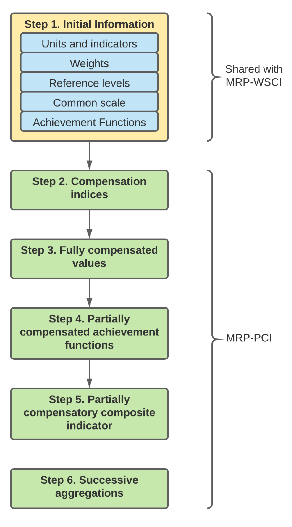
The process to build this partially compensatory indicator () has 6 steps (see Figure 1). The first one is shared with the MRP-WSCI methodology [4] (see details about the construction of the weak, , strong, , and mixed, , composite indicators in Appendix A) and contains the basic initial information of the reference point based procedure. Let us describe the steps in detail.
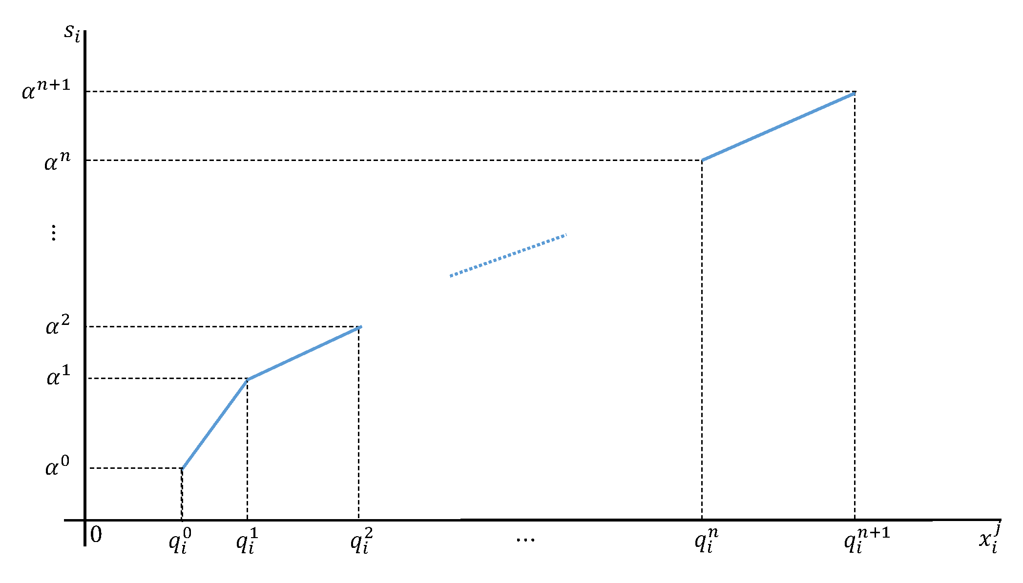
- Initial information: it will be assumed that we are managing a set of J units, for which I indicators are evaluated, which, without loss of generality, will all be assumed to be of type “the more, the better”. Let us denote by the value of indicator i for unit j. It will also be assumed that the decision maker has somehow assigned weights to the indicators, which reflect the contribution of each indicator to the final composite measure.It is also assumed that the decision maker can give, for each indicator i, n reference levels, , which somehow define the performance levels of indicator i (e.g., very poor, poor, fair, good, very good,...). Let us denote by and , respectively, the minimum and maximum values that indicator i can take. Therefore, we obtain the following -dimensional reference vector for indicator i:We will also assume that a set of real values is available (either provided by the decision maker or set to default values by the analysts), which define the common measurement scale. Note that these values are the same for all the I indicators. Therefore, each () is the value in the common scale that a given unit has if it achieves value in indicator i. In order to turn each indicator i to the scale defined by the values (), a so-called achievement function is used, which, apart from allowing the normalisation of the indicators, also informs about the relative position of each unit with respect to the reference levels given in the previous step, for the corresponding indicator. These functions were originally defined in [29] for general reference point procedures (with one reference level), and they were afterwards extended to double reference point methods [30], and adapted to the calculation of composite indicators [28,34,35]. This achievement function is generalized to the case when n reference levels are used in the following way:Therefore, the achievement function of indicator i is a piece-wise linear function that takes values between and if the unit achieves values between and for indicator i (see Figure 2). It must be noted that the distance-based normalization proposed for the MRP-WSCI methodology is more general than other schemes, meaning that others can be obtained as particular cases of this one. For example the well known range normalization is obtained for , , .All the previously described basic initial elements are shared with the MRP-WSCI methodology, which is described in Appendix A.
- Compensation indices: the main feature of this partially compensatory indicator is allowing the decision maker to provide a compensation index for each indicator. is understood as a coefficient, between 0 and 1, which indicates to what extent can a bad value of indicator i be compensated by better values of other indicators.
- Fully compensated values: given all the previous data, let us build now the fully compensated value of each indicator i for each unit j, , which is the weighted average of and the rest of achievement function values that are at least as good as . As a result, the value of is fully compensated by all the better (or equal) values of the rest of indicators:where is the subset of indicators that take a value better or equal to indicator i for unit j:
- Partially compensated achievement scalarizing functions: next, we combine the compensation indices given in Step 2 with the fully compensated values of Step 3, to obtain the partially compensated achievement scalarizing functions, . These functions measure the partially compensated value of each indicator i for each unit j, taking the compensation indices into account:is a value lying between the original achievement scalarizing function, , and the fully compensated value, , of indicator i for unit j, according to the corresponding compensation index of indicator i, . Therefore, if , then takes the value of the achievement function . On the other hand, if , then takes the value of the fully compensated value of indicator i, .
- Partially compensatory composite indicator: finally, the partially compensatory indicator of unit j is defined as the worse (minimum) of the partially compensated achievement scalarizing functions of unit j as follows:
- Successive aggregations: in many real cases, the system of indicators is organized in several levels. For example, in the environmental sustainability assessment reported in Section 4, the indicators are classified in families. Therefore, the process has two stages. First, the indicators of each family are aggregated, and we obtain the partially compensatory composite indicator for each of them. Given the way they have been constructed, take values in the same scale as the original achievement functions and therefore, they can be used as achievement functions in a multi-stage aggregation process. Thus, in a second stage, we use these composite indicators as achievement functions to build the global composite indicators and so on. This is important, because it may make sense to provide different compensation indices depending on the aggregation stage. For example, when assessing sustainability, indicators of the same family may be compensated, but not the families among them.
3.2. Theoretical Properties of the MRP-PCI Indicators
Let us consider a given unit , and let us assume, without loss of generality, that the indicators are ordered according to the values of the achievement functions:
The following properties can be easily proved:
- coincides with the weak composite indicator , defined in (A2):
- The fully compensated values satisfy:
- For all , it holds that and, therefore:
Making use of these properties, let us state the significant relationships between the indicator with the original MRP-WSCI indicators (described in Appendix A), that is, with the weak, (A2), un-weighted strong, (A3) and mixed, (A4) composite indicators:
- and, if , then :
- and, if , then :
- If , then :
As a result, it has been proved that always lies between the weak composite indicator and the un-weighted strong composite indicator . In general, it will be closer to when the worst indicators of unit j are not compensable (their corresponding are zero), and closer to when the worst indicators of unit j are fully compensable (their corresponding are one). Moreover, the MRP-PCI method has been proven to generalize the MRP-WSCI scheme, given that and are particular cases of , when the compensation indices of all the indicators are equal to 1 and 0, respectively, and is a particular case of , when the compensation indices of all the indicators are equal to . Therefore, the MRP-PCI method offers a wider and more flexible modelling scheme by allowing the decision maker to use different compensation indices for each indicator.
3.3. A Hypothetical Example
In order to illustrate the practical meanings of the variables used, and the effect of the compensation indices in the partially compensatory indicator , let us consider a hypothetical case with three indicators. As an example of compensation indices, a not too hard way of assessing these values would be using a three value scale (of course, a decision maker can give more values between 0 and 1 if so desired):
- , no compensation: a bad value of indicator i cannot be compensated in any way.
- , full compensation: a bad value of indicator i can be completely compensated by better values in other indicators.
- , middle compensation: a bad value of indicator i can be partially (half) compensated by better values in other indicators.
Let us assume that indicator 1 can be fully compensated (), indicator 2 can be partially compensated () and indicator 3 cannot be compensated at all (). For simplicity, we will assume that all the three indicators are equally weighted. Let us also assume that we are considering 4 units, and that the achievement function is measured in a 0–1–2–3 scale (which corresponds to 2 reference levels). The hypothetical values of the achievement scalarizing functions, the resulting values of the MRP-PCI partially compensatory composite indicators and the values of the MRP-WSCI weak, strong and mixed (for ) composite indicators, can be seen in Table 1. The intermediate calculations needed to build , that is, the fully compensated value of each indicator for each each unit () and the partially compensated achievement scalarizing function (), can be seen in Table 2.
Let us explain the results of the first row of Table 2. The worst value of unit 1 takes place in indicator 1, and therefore, is the average of the three achievement scalarizing function values of unit 1. Similarly, indicator 2 is the second best for unit 1, and therefore, is the average value of and . Finally, indicator 3 gets the best value for this unit and thus, . Given that indicator 1 can be fully compensated, . On the other hand, indicator 2 can be only partially compensated and therefore, is half way between and . Finally, given that indicator 3 cannot be compensated at all, . For the first three units, it holds that the worst partially compensated achievement scalarizing function value is achieved by the indicator with the worst achievement function value . Under these circumstances, we can explain the results of the composite indicators obtained in Table 1. Given that , the partially compensatory composite indicator of unit 1 gets the fully compensated value, that is, , and given that , the partially compensatory composite indicator of unit 3 gets the no compensatory value, that is, . Given that the MRP-WSCI mixed indicator needs to use the same compensation index for all the indicators, it is not able to take into account these different compensation indices of indicators 1 and 3, and . On the other hand, and therefore, is half way between and . In this case, , because . These can be regarded as extreme cases, but other intermediate situations can take place. The worst value of unit 4 takes place in indicator 1, as happens with unit 1. However, once compensated according to the different compensation indices, the worst partially compensated achievement scalarizing function value corresponds to indicator 3, and therefore, . In this case, similarly to unit 1, . Therefore, the MRP-PCI method successfully takes into account the different compensation indices assigned to the indicators, and produces the final composite indicators accordingly. Besides, if different weights were considered for the indicators, the results could also be different.
In Section 4, we apply the partially compensatory indicator to the assessment of the environmental sustainability of the provinces of the Spanish southern region of Andalucía, and we discuss the results obtained, comparing them with the MRP-WSCI weak and strong composite indicators.
4. Example: Applying the MRP-PCI Method to an Environmental Sustainability Assessment Case
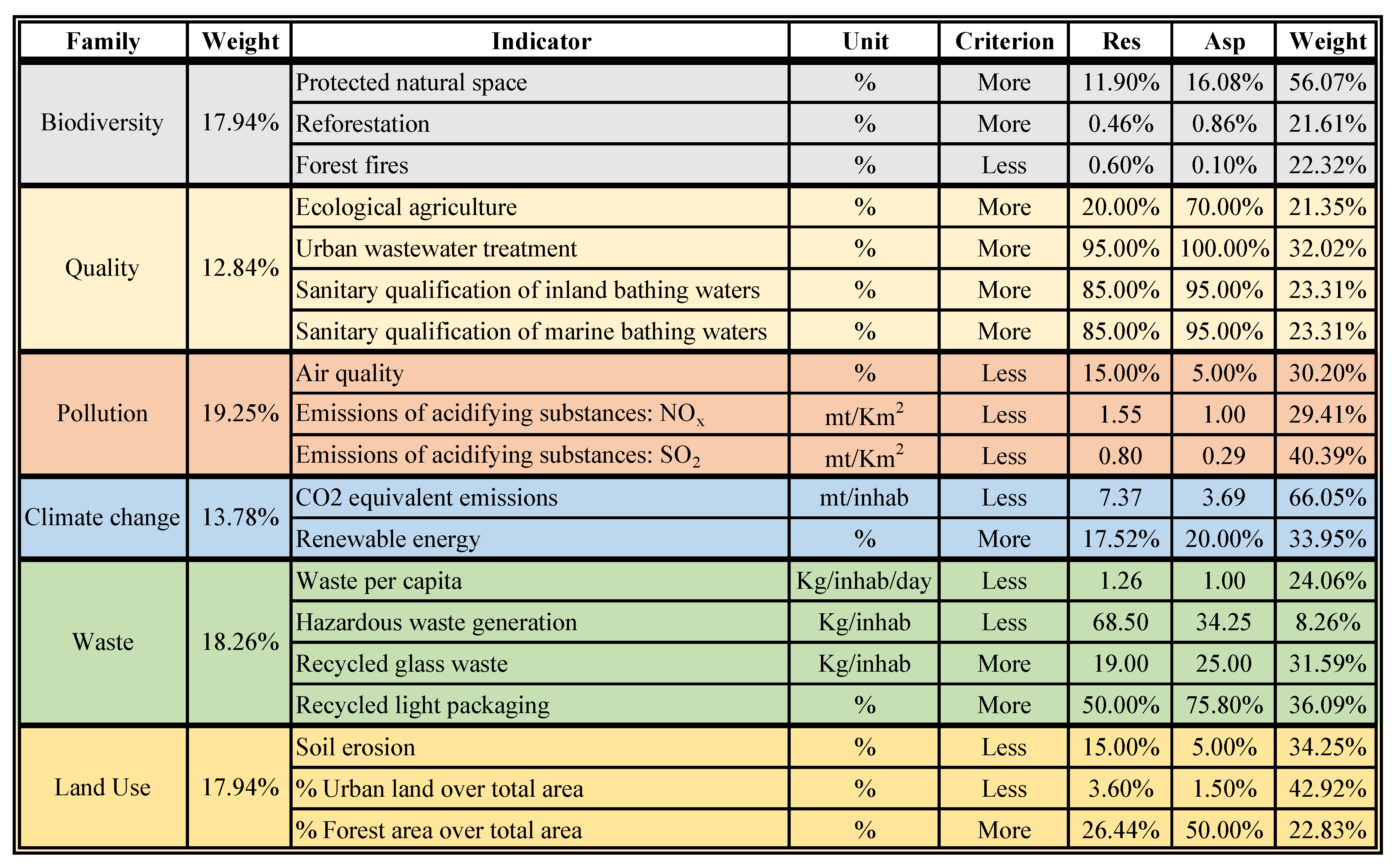
To illustrate the application of the partially compensatory composite indicator to sustainability assessment problems, we used the data given by [33], to assess the environmental sustainability of the eight provinces of the Spanish southern region of Andalucía. In that paper, the MRP-WSCI methodology was used to determine the weak and strong composite environmental sustainability indicators of the regions. The aim of this section is to compare these results with the ones obtained using the MRP-PCI method, and to study the practical effect of the compensation indices and the subsequent partially compensatory aggregation scheme. In this study, 19 single indicators were used, which are grouped into six families. The data of the indicators were obtained from the Regional Ministry of Environment and Land Management of the Andalusian Government and from the Andalusian Energy Agency. Besides, a panel of experts gave two absolute reference levels (named as reservation and aspiration levels) for each indicator, based on their own expertise, and they also assigned weights to the single indicators and to the families. All these data can be seen in Figure 3.
Given that two reference levels were used, the achievement functions took values in a 0–1–2–3 scale. Therefore, a value between 0 and 1 means that the corresponding indicator performed worse than the corresponding reservation level, a value between 1 and 2 means that the indicator performed between the reservation and aspiration levels, and a value over 2 means that the indicator performed better than the aspiration level. Besides, two aggregations were made. First, the single indicators of each family were aggregated, to obtain the family composite indicators of each province. Second, family indicators were aggregated to obtain the global composite indicator of each province. Next, we compared the results obtained using the proposed MRP-PCI method, described in Section 3, with the strong and weak MRP-WSCI indicators, as described in Appendix A, for both aggregations. To this end, we used hypothetical compensation indices for different indicators and families, in order to illustrate how the partially compensatory method behaves. Therefore, it must be pointed out that the specific results obtained are not necessarily significant as sustainability measures, given that the compensation indices have been assigned with illustrative purposes, and not by experts in the field.
4.1. Aggregation 1
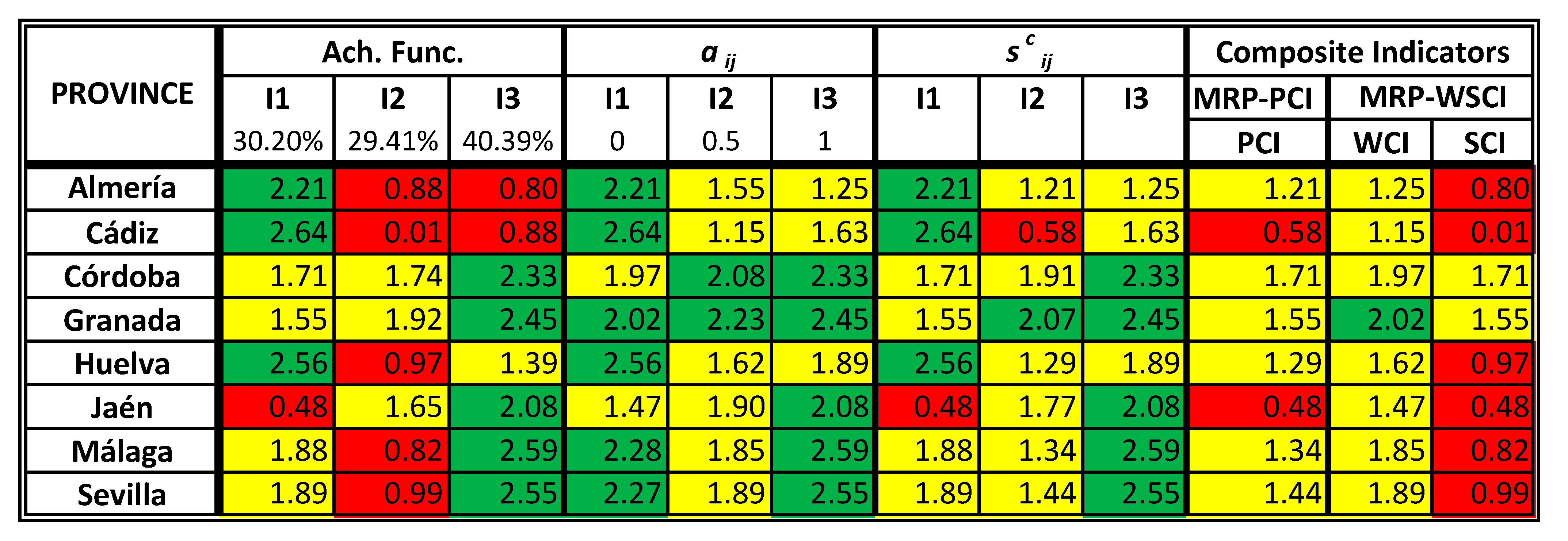
As a first example, let us build the partially compensatory composite indicator for the Pollution family, using the MRP-PCI method. To this end, we assumed that the decision makers regard Air quality (I1) as non-compensable (), Emissions of NO (I2) as partially compensable () and Emissions of SO (I3) as fully compensable (). Once again, note that these were hypothetical indices, just to illustrate the way the works. Figure 4 shows the results obtained for this family. In the first block, we can see the values of the achievement functions of the three indicators, with a color code (green for values over 2, that is, better than the aspiration level; yellow for values between 1 and 2, that is, between the reservation and aspiration levels; and red for values under 1, worse than the reservation level). The second and third blocks contain, respectively, the fully compensated value of each indicator (), and the partially compensated achievement scalarizing function (), necessary for the calculation of the . Finally, the last block shows the values of the partially compensatory indicators (), and those of the MRP-WSCI weak () and strong () composite indicators, in order to compare them.
Comparing the results of the with those of the and indicators, three different cases can be seen in Figure 4:
- For three provinces (Córdoba, Granada and Jaén), the partially compensatory indicator coincided with the strong composite indicator. This is because in the three cases, the worst performance of the family took place in the Air quality (I1) indicator, which cannot be compensated at all.
- In four provinces (Cádiz, Huelva, Málaga and Sevilla), the had an intermediate value between and , not close to any of them. In this case, the worst performance took place in the Emissions of NO (I2) indicator, which was partially compensable.
- Finally, for Almería, the was much closer to the , because its worst performance took place in the Emissions of SO (I3), which was fully compensable.
Therefore, it can be seen that the results, as desired, reflect the compensation indices given to the different indicators. For simplicity reasons, for the rest of the families, the first aggregation has been carried out assuming full compensation for all the indicators (that is, in these cases, the equals the for all the provinces).
4.2. Aggregation 2
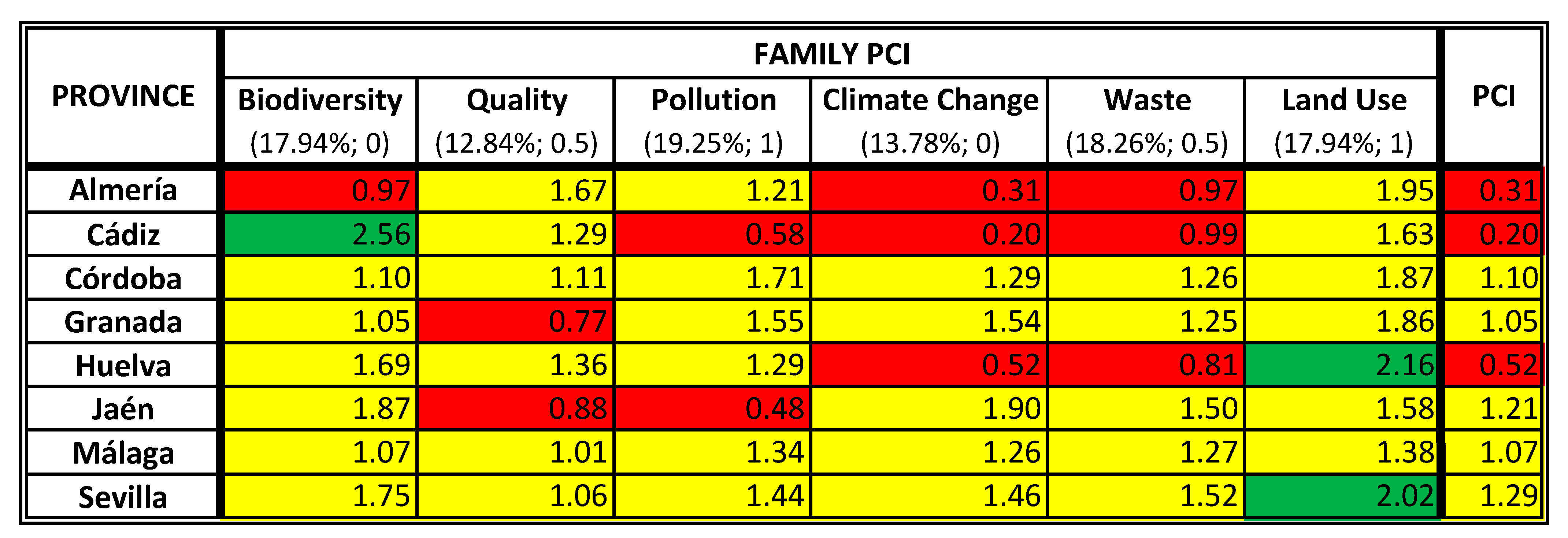
Once we have calculated the composite indicators for each family, we carried out a second aggregation to obtain the global indicators, using the family weights specified in Figure 3. First, we obtained the global partially compensatory composite indicators, using the proposed MRP-PCI method. Then, we calculated the weak and strong indicators obtained using the MRP-WSCI methodology, and we compared the results of this second aggregation.
4.2.1. The MRP-PCI Composite Indicator
For the global , we used the indicators of each family. Let us remind that we only used different compensation indices in the Pollution family, while full compensation was allowed in the rest of them. As for the compensation indices for the families, again as an illustrative example, we allowed full compensation (1) for Pollution and Land Use, partial compensation (0.5) for Quality and Waste and no compensation (0) for Biodiversity and Climate Change. The final results obtained for the global indicator can be seen in Figure 5. Sevilla got the best global composite indicator, because all the families performed better than their reservation levels and one of them (Land Use) performed better than the aspiration level. It was closely followed by Jaén, that gets the second best result, despite the fact of having two families (Quality and Pollution) under their reservation levels. This is so because Quality could be partially compensated and Pollution could be fully compensated by the better values of the rest of the families. Córdoba, Málaga and Granada also get global indicators over the reservation level. Huelva, Almería and Cádiz got global values under the reservation level. This is because they all performed worse than the reservation levels for families that could not be compensated at all.
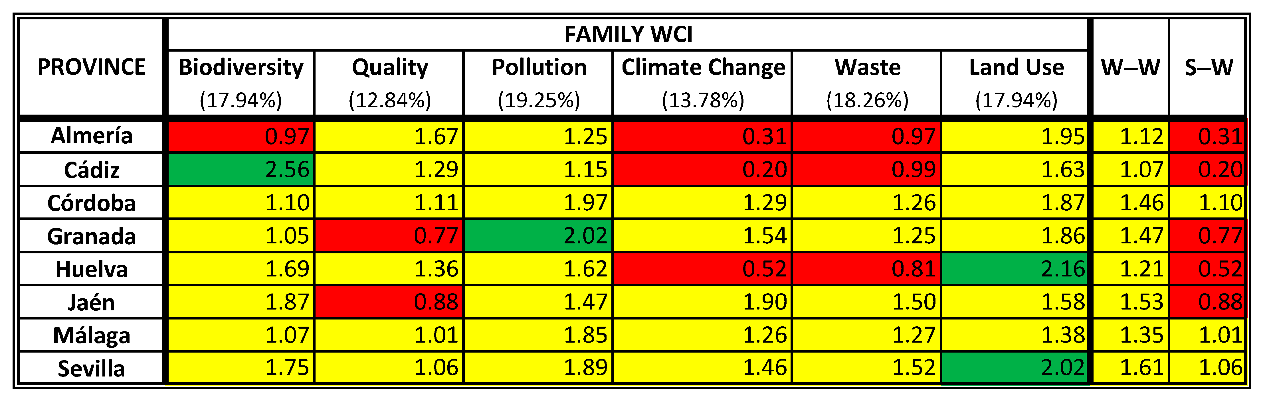
4.2.2. MRP-WSCI Composite Indicators
For this second aggregation, let us use the of each family as achievement functions, as described in Appendix A. This way, we could obtain the weak-weak () and the strong-weak () global composite indicators (Figure 6). As can be seen, the indicator showed an intermediate overall behavior (between the global reservation and aspiration levels) for all the provinces, when full compensation is allowed. On the other hand, the indicator means that Almería, Cádiz, Granada, Huelva and Jaén performed worse than the reservation level for at least one family, while Córdoba, Málaga and Sevilla performed better than the reservation level in all the families.
4.2.3. Comparison of the Results
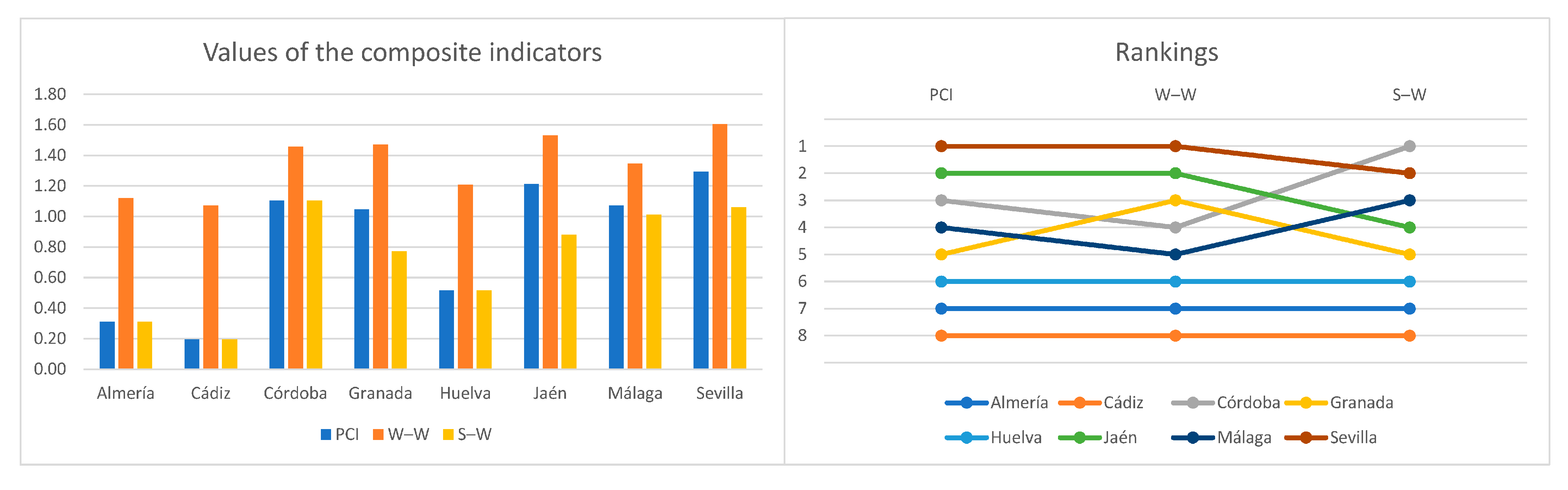
Let us compare the results obtained for the partially compensatory indicator (Figure 5), with the and indicators of Figure 6. We can see that the gets the same value as the indicator for Almería, Cádiz, Córdoba and Huelva. This is because, in all these cases, the worst family in Figure 5 was Climate Change, which could not be compensated at all. On the other hand, for Granada, Málaga and Sevilla, the lay between their corresponding and indicators. In all these provinces, the worst performance took place in the Quality family, which could be partially compensated. Finally, Jaén had the worst performance in the Pollution family, which, as previously mentioned, could be fully compensated. This is why its improved significantly with respect to the composite indicator, and this province even overtook Málaga in the score.
Taking the previously mentioned comments into account, we can conclude that the global was successfully capable of incorporating the nuances generated by the various compensation indices assigned to the indicators and families. Besides, if we had allowed different compensation indices within the rest of families, the results would have been more varied. Moreover, two other important advantages of the could be observed:
- Let us take a look at Figure 7, where the values of the , and indicators (left) and the rankings provided by them (right) are compared. As can be seen, the got an intermediate position between the fully compensatory and non-compensatory indicators, thus showing a less extreme behavior. In [4], it is argued that the joint use of the weak and strong indicators provides useful additional information. However, if a single composite indicator needs to be used, for example for ranking purposes, then the can be a more balanced option.
- If we look at the variation ranges (between the minimum and the maximum values) of the composite indicators in Figure 5 and Figure 6, we can see that, for this example, the variation of the (1.1) was greater than these of the rest (: 0.53; : 0.91). Therefore, it seems that the hasd a greater dispersion than the others, which allowed a better distinction among the performances of the different provinces.
5. Discussion: Interesting Features of the MRP-PCI Method
Let us discuss some interesting features about the MRP-PCI method and its potential application to real problems. As seen, the method needs a number of preferential parameters (weights, reference levels and compensation indices) to be assessed. This may bring about two criticisms to the method. First, it can be argued that the final results are too dependent on subjective parameters given by the decision maker. Second, it can also be argued that this places a too high cognitive effort on the decision maker. With respect to the first issue, we would like to point out that, in our opinion, there is no such thing as a “fully objective” aggregation methodology to build composite indicators. There is always some subjectivity, either explicitly stated, or implicitly assumed (or even hidden). For example, a methodology that does not use weights may assume in practice an equal weighting scheme, which is even more arguable. Or even some pure statistical approaches do in practice imply assumptions about which indicators have more relevance (that is, weight) in the final measure, which are many times unknown (and therefore, not agreed upon) by the decision makers. In our opinion, it is not a question of trying to be objective, but rather than that, of clearly identifying the subjective elements of the model and interpreting the results based on them. It is each user who must include her/his own preferential information, which logically may yield to different final results. We believe that the MRP-PCI method succeeds in this regard. With respect to the second issue, is all this information too hard to be provided by the decision maker? Regarding the weights, they are necessary for our approach, as they are for many others, and there are many ways proposed in the scientific literature to assess them according to the decision maker’s tastes (see, e.g., [14,36]). Regarding the reference levels, as discussed in [4], they can be established in two ways. First, they can be given by the decision makers or set by panels of experts (“absolute levels”), if they have enough knowledge about the problem and they wish to do so. We agree that this may be hard in certain problems, but, as seen in this paper, if it is possible to give them, they add value to the method, and the results give us an absolute measure of performance, with respect to these values. Alternatively, if this option is not possible, they can be set statistically, given a data set (“relative levels”). In this case, the cognitive burden is not significant, and the results measure the relative position of the units with respect to those belonging to the data set. In both cases, but especially if relative reference levels are used, it is necessary to analyze if there are outliers which could bias the results and to use robust measures for such levels. The discussion about this issue given in [4] is naturally valid for the MRP-PCI scheme. Anyway, it must be pointed out that, in the case when no reference levels are available, our proposed scheme can be adapted and contains, for example, the well known range normalization as a particular case. Therefore, the partially compensatory scheme proposed in this paper can be used even if the decision makers do not wish to establish these reference levels.
Let us discuss now about the compensation indices. While it may seem harder to provide these indices for every single indicator (and family), we believe that their interpretation is much more intuitive for the decision maker than a single global compensation index (like parameter in the MRP-WSCI mixed indicator, see Appendix A), although the same index can be used for every indicator if so desired. As previously mentioned, when assessing sustainability, it is certainly sensible to think that decision makers may want to assess different compensation indices to the different indicators, or to compensate differently, for example, among single indicators of a family or among the families themselves. Besides, a scale like the three values suggested in the paper (no compensation, partial compensation, full compensation) may not be too uncomfortable. Of course, any user can give more intermediate values if so desired. One may think that weights and compensation indices should have a strong relationship, that is, the more important an indicator is regarded, the less it can be compensated. While this can be the case in some occasions, we believe it is not always necessarily this way. For example, when evaluating projects, decision makers may set a minimum performance on the safety indicator under which a project is not acceptable (therefore, a bad performance in this indicator cannot be compensated by good performances in others), but its weight on the final score (provided that this minimum is achieved) is not higher than others like price, technical soundness, etc. Nevertheless, in a real application, a sensitivity analysis on the different parameters of the method should always be carried out to establish the robustness of the results obtained.
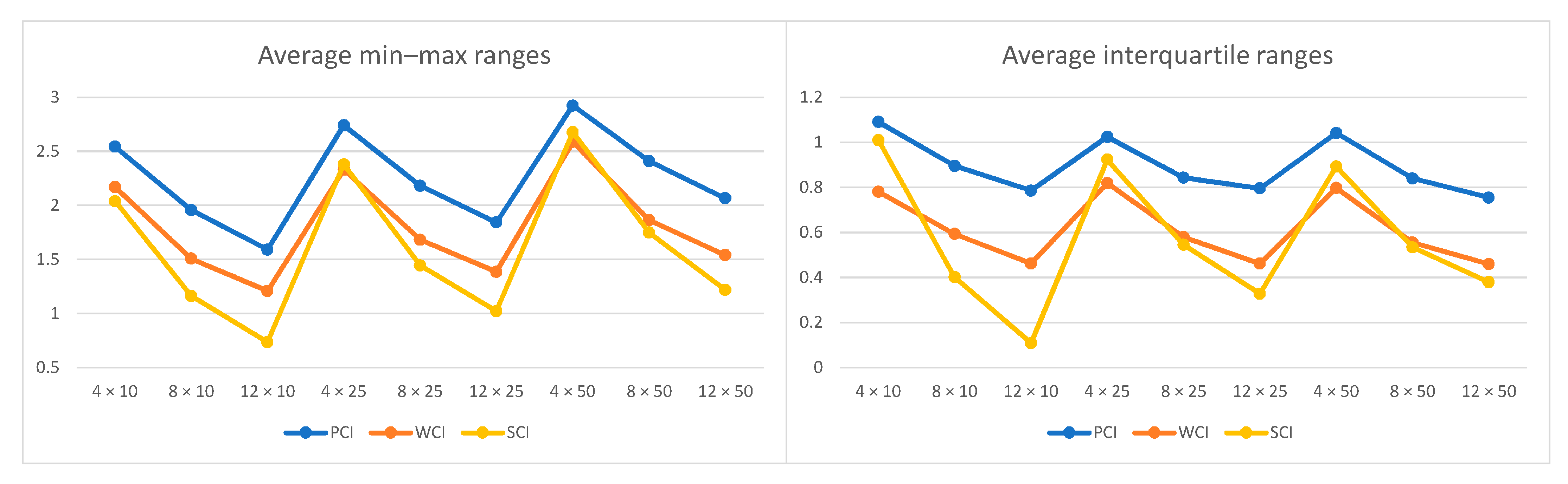
While the weak and strong composite indicators of the MRP-WSCI scheme, jointly visualized, provide a very useful information for decision makers about the performance of the units, their extreme compensability nature (full compensation or no compensation at all, respectively) may make them less suitable for ranking purposes. As seen in this paper, the MRP-PCI indicator is usually less extreme, and takes values in a wider range, which allows ranking in a more effective way. In order to test whether this is generally the case, we have conducted a series of computational experiments (numerical results are available upon request to the authors.). To be more precise, we have generated combinations of systems of indicators with 4, 8 and 12 indicators and with 10, 25 and 50 units. For each of the nine combinations, we have generated 100 different systems. Therefore, a total of 900 experiments have been carried out. For each of them, the values of the single indicators for the different units (values between 0 and 100) and their compensation indices (values 0, 0.5 or 1) have been randomly generated. Then, the corresponding partially compensatory (), weak () and strong () composite indicators have been calculated for each unit. For each combination of numbers of indicators and units, we have calculated the average range (across the 100 experiments) between the maximum and minimum values of each of the three composite indicators, as well as the average interquartile ranges. The results can be seen in Figure 8. As seen, the average ranges of the are always greater than those of the and the composite indicators.
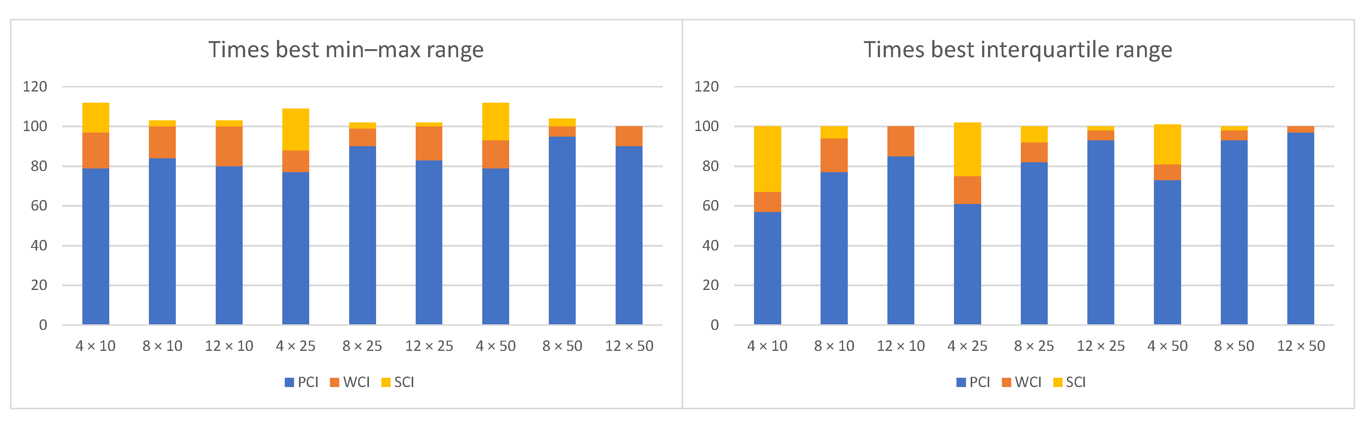
Besides, for each of the nine combinations, we have counted the number of times (across the 100 experiments) that each composite indicator has the greatest range. The results are shown in Figure 9 (some columns add up to more than 100 because there are ties in the first position). As seen, in all cases, the has the greatest range in a wide majority of the experiments. Finally, we have checked the position of the median values of the composite indicators, and we have found out that in every single experiment, the median of the lies between the medians of the and the .
6. Conclusions
In this paper, we have developed a method to build partially compensatory composite indicators, named as MRP-PCI. This is a methodological contribution that can be used to build these composite indicators for any system of indicators within any field. In particular, in the sustainability assessment field, any type of sustainability can be assessed, provided that an adequate system of indicators measuring it is available. Compensability is a crucial aspect in sustainability assessment, and the method developed offers a way to handle this issue according to the wishes of the decision makers. More precisely, the main contributions of this paper are:
- The method allows the possibility to provide a different compensation index for each indicator, or for each of the families into which the indicators are grouped in successive aggregations. To the best of our knowledge, this is the first composite indicator method that allows this possibility. It is sensible to think that the decision center may regard different indicators as differently compensable, and if there are several aggregation levels, the compensations may not be the same at each level. Therefore, this formulation offers a high modelling flexibility, because the decision maker can decide which indicators can be compensated and to which extent. Given that sustainability indicators are usually classified into different areas (economic, social, environmental), and the compensation among them is a critical issue when assessing the global sustainability of a territory, the MRP-PCI method is specially suitable in this field.
- An aggregation method has been designed that takes all these compensation indices into account, to build a partially compensatory composite indicator. Using an illustrative example about the environmental sustainability assessment, we have shown how this approach works when different compensation indices are established in a problem with two aggregation levels. As seen, the results successfully reflect these compensation indices in an intuitive and easy-to-interpret way.
- The MRP-PCI method is based on the multiple reference point, MRP-WSCI, scheme. Therefore, it is assumed that the decision maker can provide reference levels for each indicator, and an achievement function is used to measure the position of each unit with respect to these levels. Nevertheless, the aggregation process followed to build the partially compensatory indicator is different and more general. In fact, it has been seen that the original weak and strong indicators built using the MRP-WSCI methodology can be obtained as particular cases of the partially compensatory composite indicator.
- A series of computational experiments have been carried out to compare the new MRP-PCI composite indicator with the MRP-WSCI weak and strong indicators. As a result, the two following interesting findings have been derived, that make the partially compensatory indicator suited for ranking purposes, when full compensation is not allowed, which is usually the case in sustainability assessment problems:
- -
- The MRP-PCI method tends to produce results with an intermediate position between the weak and the strong composite indicators, thus showing a less extreme behavior.
- -
- The MRP-PCI method very frequently has a greater dispersion than the others, which allows a better distinction among the performances of the different units.
Moreover, this paper opens a research line that allows to develop partially compensatory versions of other existing methodologies. In fact, it is not hard to adapt the method proposed to other composite indicators building procedures, by using their corresponding normalized assessments instead of the achievement function used in the reference point based methods. Anyway, we have discussed that, not only the original MRP-WSCI indicators, but others using different (not necessarily based on the use of reference levels) normalizations, can be regarded as particular cases of the MRP-PCI method. Therefore, the method developed provides a flexible enough methodological framework that can be adapted to each particular problem, and to the specific wishes of the decision makers.
Author Contributions
Conceptualization, J.M.C. and F.R.; methodology, J.M.C. and F.R.; software and computational experiments, J.M.C.; writing—original draft preparation, F.R.; writing—review and editing, J.M.C. and F.R.; visualization, J.M.C. and F.R.; supervision, F.R. All authors have read and agreed to the published version of the manuscript.
Funding
This research was partially funded by Spanish Ministry of Economy and Competitiveness (Project PID2019-104263RB-C42), from the Regional Government of Andalucía (research group SEJ-417), and by the EU ERDF operative program (project UMA18-FEDERJA-065).
Data Availability Statement
The results of the simulations are available in the following repository: http://webpersonal.uma.es/~rua/english/Repository/repository.html.
Conflicts of Interest
The authors declare no conflict of interest. The funders had no role in the design of the study; in the collection, analyses, or interpretation of data; in the writing of the manuscript, or in the decision to publish the results.
Abbreviations
The following abbreviations are used in this manuscript:
| MCI | Mixed composite indicator |
| MRP-PCI | Multiple reference point partially compensatory indicator |
| MRP-WSCI | Multiple reference point weak and strong composite indicators |
| PCI | Partially compensatory composite indicator |
| SCI | Strong composite indicator |
| S-S | Strong-strong global composite indicator |
| S-W | Strong-weak global composite indicator |
| WCI | Weak composite indicator |
| W-W | Weak-weak global composite indicator |
Besides, the following notation is used for the variables and parameters that appear in the description of the MRP-PCI method developed:
| Fully compensated value of of indicator i for unit j | |
| t-th value of the common measurement scale | |
| I | Number of indicators (i is the corresponding index) |
| Subset of indicators with a value better or equal to indicator i for unit j | |
| J | Number of units (j is the corresponding index) |
| Compensation index assigned to indicator i | |
| Weight assigned to indicator i | |
| n | Number of reference levels (t is the corresponding index) |
| Normalized weight of indicator i | |
| Partially compensatory composite indicator of unit j | |
| t-th reference level of indicator i | |
| Value of the scalarizing achievement function of indicator i for unit j | |
| Partially compensated achievement scalarizing function of indicator i for unit j | |
| Value of indicator i for unit j |
Appendix A. The MRP-WSCI Composite Indicators
For readability reasons, and in order to obtain a self-contained paper, we summarize in this appendix the description of the construction process of the MRP-WSCI composite indicators given in [4]. As for the MRP-PCI method, let us consider J units and I indicators (all of them of type “the more, the better”). denotes the value of indicator i for unit j. Let us consider the following elements, which are also common to the MRP-PCI method:
- The weights for the indicators.
- The reference vector , expressing performance levels of the indicators.
- The common measurement scale .
- The corresponding achievement scalarizing functions, as defined in (2).
The weak composite indicator () uses an additive aggregation, which allows compensation among the single indicators. In order to build it, the weights are normalized to add up to 1:
Making use of weights (A1) and achievement function (2), the of a given unit j is built using a simple additive weighted aggregation:
The strong composite indicator () does not allow any compensation and there are two options to build it. The simplest way (un-weighted ) is not to consider weights, and just to take the value of the worst achievement function:
On the other hand, if the weights are considered, [4] provide a way to build the weighted which is designed to be in the same sub-interval as the worse indicator of unit j, to take a worse value if the corresponding indicator has a higher weight, and in particular, to take the worst possible value if unit j has the worst possible value in the highest weighted indicator. Therefore, the weighted measures the worst performance of unit j, relativized by the weights of the indicators. The unweighted version is used in this paper and therefore, the readers are referred to the above publication for further details on the weighted version.
As it happens with , both and take values in the same scale as the original achievement functions and therefore, they can be used as achievement functions in a multi-stage aggregation process. If the weak composite indicators are used as achievement functions, we can get the global weak-weak composite indicator (denoted as ), which is a global compensatory measure, and the global strong-weak composite indicator (denoted as ), which points out the worst family of each unit. Alternatively, the strong composite indicators of each family can be used as achievement functions in the second stage. In this case, it is interesting to consider the strong-strong global indicator (denoted as ), which points out the worst individual indicator.
As previously mentioned, the weak composite indicator has the properties of the classical weighted means, and thus good performances in certain indicators can compensate bad performances in others (to this end, it is assumed that the single indicators are mutually preferentially independent [37]). On the other hand, the strong composite indicator does not allow any compensation among the indicators, and it just takes the value of the worst performance of unit j. Therefore, and represent two extreme cases: no normalization and full normalization, respectively. In [4], an intermediate (mixed) composite indicator is also proposed, for different compensation degrees. If the compensation degree is denoted by , with , then the mixed indicator of unit j is defined as:
Therefore, means no compensation (and we get the value of the strong indicator), while means full compensation (and we get the value of the weak indicator). Nevertheless, this mixed indicator has two main drawbacks. First, the value of is difficult to be interpreted, and thus assessed, by a decision maker, because it is just the coefficient of a convex combination between and . Second, is a general compensation degree, that is, it does not allow the decision maker to assess different compensation degrees to different indicators.
References
- Mori, K.; Yamashita, T. Methodological framework of sustainability assessment in City Sustainability Index (CSI): A concept of constraint and maximisation indicator. Habitat Int. 2015, 45, 10–14. [Google Scholar] [CrossRef]
- Sala, S.; Ciuffo, B.; Nijkamp, P. A systemic framework for sustainability assessment. Ecol. Econ. 2015, 119, 314–325. [Google Scholar] [CrossRef]
- Munda, G. Social Multi-Criteria Evaluation for a Sustainable Economy; Springer: New York, NY, USA, 2008. [Google Scholar]
- Ruiz, F.; Gibari, S.E.; Cabello, J.M.; Gómez, T. MRP-WSCI: Multiple Reference Point based Weak and Strong Composite Indicators. Omega 2020, 95, 102060. [Google Scholar] [CrossRef]
- Komiyama, H.; Takeuchi, K. Sustainability Science: Building a New Discipline. Sustain. Sci. 2006, 1, 1–6. [Google Scholar] [CrossRef]
- United Nations. Report of the World Commission on Environment and Development “Our Common Future”. 1987. Available online: https://sustainabledevelopment.un.org/content/documents/5987our-common-future.pdf (accessed on 5 December 2020).
- Atkinson, G.; Dubourg, R.; Hamilton, K.; Munashinghe, M.; Pearce, D.; Young, C. Measuring Sustainable Development: Macroeconomics and the Environment; Edward Elgar Publishing: Cheltenham, UK, 1997. [Google Scholar]
- United Nations. Transforming Our World: The 2030 Agenda for Sustainable Development. 2015. Available online: https://sustainabledevelopment.un.org/post2015/transformingourworld (accessed on 10 December 2020).
- Neumayer, E. Weak Versus Strong Sustainability: Exploring the Limits of Two Opposing Paradigms; Edward Elgar Pub: Cheltenham, UK, 2010. [Google Scholar]
- Chaminade, C. Innovation for what? Unpacking the role of innovation for weak and strong sustainability. J. Sustain. Res. 2020, 2, e200007. [Google Scholar]
- Nasrollahi, Z.; Hashemi, M.S.; Bameri, S.; Taghvaee, V.M. Environmental pollution, economic growth, population, industrialization, and technology in weak and strong sustainability: Using STIRPAT model. Environ. Dev. Sustain. 2020, 22, 1105–1122. [Google Scholar] [CrossRef]
- Binder, C.L.; Wyss, R.; Massaro, E. (Eds.) Sustainability Assessment of Urban Systems; Cambridge University Press: Cambridge, UK, 2020. [Google Scholar]
- Saisana, M.; Tarantola, S. State-of-the-Art Report on Current Methodologies and Practices for Composite Indicator Development; Technical Report; Joint Research Centre, European Commission: Ispra, Italy, 2002. [Google Scholar]
- Nardo, M.; Saisana, M.; Saltelli, A.; Tarantola, S. Tools for Composite Indicators Building; Technical Report; European Commission: Ispra, Italy, 2005. [Google Scholar]
- Singh, R.K.; Murty, H.R.; Gupta, S.K.; Dikshit, A.K. An overview of sustainability assessment methodologies. Ecol. Indic. 2009, 9, 189–212. [Google Scholar] [CrossRef]
- Gana, X.; Fernandez, I.; Guo, J.; Wilson, M.; Zhao, Y.; Zhou, B.; Wu, J. When to use what: Methods for weighting and aggregating sustainability indicators. Ecol. Indic. 2017, 81, 491–502. [Google Scholar] [CrossRef]
- Yi, P.; Wang, L.; Zhang, D.; Li, W. Sustainability Assessment of Provincial-Level Regions in China Using Composite Sustainable Indicator. Sustainability 2019, 11, 5289. [Google Scholar] [CrossRef] [Green Version]
- Ciommi, M.; Gigliarano, C.; Emili, A.; Taralli, S.; Chelli, F.M. A new class of composite indicators for measuring well-being at thelocal level: An application to the equitable and sustainable Well-being (BES) of the Italian provinces. Ecol. Indic. 2017, 76, 281–296. [Google Scholar] [CrossRef]
- Painii-Montero, V.F.; Santillán-Muñoz, O.; Barcos-Arias, M.; Portalanza, D.; Durigon, A.; Garcés-Fiallos, F.R. Towards indicators of sustainable development for soybeans productive units: A multicriteria perspective for the Ecuadorian coast. Ecol. Indic. 2020, 119, 106800. [Google Scholar] [CrossRef]
- De Montis, A.; Serra, V.; Ganciu, A.; Ledda, A. Assessing landscape fragmentation: A composite indicator. Sustainability 2020, 12, 9632. [Google Scholar] [CrossRef]
- El Gibari, S.; Gómez, T.; Ruiz, F. Building composite indicators using multicriteria methods: A review. J. Bus. Econ. 2019, 89, 1–24. [Google Scholar] [CrossRef]
- Díaz-Balteiro, L.; Romero, C. In search of a natural systems sustainability index. Ecol. Econ. 2004, 49, 401–405. [Google Scholar] [CrossRef]
- Gómez-Limón, J.A.; Arriaza, M.; Guerrero-Baena, M.D. Building a composite indicator to measure environmental sustainability using alternative weighting methods. Sustainability 2020, 12, 4398. [Google Scholar] [CrossRef]
- Blancas, F.J.; Caballero, R.; González, M.; Lozano-Oyola, M.; Pérez, F. Goal Programming synthetic indicators: An application for sustainable tourism in Andalusian coastal counties. Ecol. Econ. 2010, 69, 2158–2172. [Google Scholar] [CrossRef]
- Tarabusi, E.C.; Guarini, G. An unbalance adjustment method for development indicators. Soc. Indic. Res. 2013, 112, 19–45. [Google Scholar] [CrossRef]
- Mazziota, M.; Pareto, A. Composite Indices Construction: The Performance Interval Approach. Soc. Indic. Res. 2020. [Google Scholar] [CrossRef]
- García-Bernabéu, A.; Hilario-Caballero, A.; Pla-Santamaría, D.; Salas-Molina, F. A process oriented MCDM approach to construct a circular economy composite index. Sustainability 2020, 12, 618. [Google Scholar] [CrossRef] [Green Version]
- Ruiz, F.; Cabello, J.M.; Luque, M. An application of reference point techniques to the calculation of synthetic sustainability indicators. J. Oper. Res. Soc. 2011, 62, 189–197. [Google Scholar] [CrossRef]
- Wierzbicki, A.P. The Use of Reference Objectives in Multiobjective Optimization. In Lecture Notes in Economics and Mathematical Systems; Fandel, G., Gal, T., Eds.; Springer: Berlin/Heidelberg, Germany, 1980; Volume 177, pp. 468–486. [Google Scholar]
- Wierzbicki, A.P.; Makowski, M.; Wessels, J. (Eds.) Model-Based Decision Support Methodology with Environmental Applications; Kluwer Academic Publishers: Dordrecht, The Netherlands, 2000. [Google Scholar]
- Acosta-Alba, I.; Van der Werf, H.M.G. The Use of Reference Values in Indicator-Based Methods for the Environmental Assessment of Agricultural Systems. Sustainability 2011, 3, 424–442. [Google Scholar] [CrossRef] [Green Version]
- Cabello, J.M.; Navarro, E.; Rodríguez, B.; Thiel, D.; Ruiz, F. Dual weak—Strong sustainability synthetic indicators using a double reference point scheme: The case of Andalucía, Spain. Oper. Res. Int. J. 2019, 19, 757–782. [Google Scholar] [CrossRef]
- Cabello, J.M.; Navarro, E.; Thiel, D.; Rodríguez, B.; Ruiz, F. Assessing environmental sustainability by the double reference point methodology: The case of the provinces of Andalusia (Spain). Int. J. Sustain. Dev. World Ecol. 2021, 28, 4–17. [Google Scholar] [CrossRef]
- Cabello, J.M.; Ruiz, F.; Pérez-Gladish, B.; Méndez-Rodríguez, P. Synthetic indicators of mutual funds’ environmental responsibility: An application of the Reference Point Method. Eur. J. Oper. Res. 2014, 236, 313–325. [Google Scholar] [CrossRef]
- Cabello, J.M.; Navarro, E.; Prieto, F.; Rodríguez, B.; Ruiz, F. Multicriteria development of synthetic indicators of the environmental profile of the Spanish regions. Ecol. Indic. 2014, 39, 10–23. [Google Scholar] [CrossRef]
- Díaz-Balteiro, L.; Belavenutti, P.; Ezquerro, M.; González-Pachón, J.; Ribeiro Nobre, S.; Romero, C. Measuring the sustainability of a natural system by using multi-criteria distance function methods: Some critical issues. J. Environ. Manag. 2018, 214, 197–203. [Google Scholar] [CrossRef]
- Munda, G.; Nardo, M. Noncompensatory/nonlinear composite indicators for ranking countries: A defensible setting. Appl. Econ. 2009, 41, 1513–1523. [Google Scholar] [CrossRef] [Green Version]
Figure 1.
Steps of the Multiple Reference Point Partially Compensatory Indicator (MRP-PCI) method. Source: own elaboration.
Figure 1.
Steps of the Multiple Reference Point Partially Compensatory Indicator (MRP-PCI) method. Source: own elaboration.

Figure 2.
Graphical representation of the achievement function. Source: [4].
Figure 2.
Graphical representation of the achievement function. Source: [4].

Figure 3.
Data of the illustrative example. Source: [33].
Figure 3.
Data of the illustrative example. Source: [33].

Figure 4.
Results for the Pollution family. Source: own elaboration.

Figure 5.
Global partially compensatory composite indicator. Source: own elaboration.

Figure 6.
Global weak–weak and strong–weak composite indicator. Source: own elaboration.

Figure 7.
Compared results and rankings. Source: own elaboration.

Figure 8.
Average min–max (left) and interquartile (right) ranges. Source: own elaboration.

Figure 9.
Times with the best min–max (left) and interquartile (right) range. Source: own elaboration.
Figure 9.
Times with the best min–max (left) and interquartile (right) range. Source: own elaboration.


Table 1.
Example: achievement functions and composite indicators.
| Indicator | Composite Ind. | ||||||
|---|---|---|---|---|---|---|---|
| Comp. Index | 1 | 0.5 | 0 | ||||
| 0.45 | 1.24 | 2.89 | 1.53 | 1.53 | 0.45 | 0.99 | |
| 2.62 | 0.14 | 2.87 | 1.01 | 1.88 | 0.14 | 1.01 | |
| 1.68 | 1.97 | 0.57 | 0.57 | 1.41 | 0.57 | 0.99 | |
| 0.45 | 2.96 | 1.23 | 1.23 | 1.34 | 0.45 | 1.90 | |
Table 2.
Example: Values of and .
| 1.53 | 2.07 | 2.89 | 1.53 | 1.65 | 2.89 | |
| 2.75 | 1.88 | 2.87 | 2.75 | 1.01 | 2.87 | |
| 1.83 | 1.97 | 1.41 | 1.83 | 1.97 | 0.57 | |
| 1.34 | 2.96 | 2.10 | 1.34 | 2.96 | 1.23 | |
Publisher’s Note: MDPI stays neutral with regard to jurisdictional claims in published maps and institutional affiliations. |
© 2021 by the authors. Licensee MDPI, Basel, Switzerland. This article is an open access article distributed under the terms and conditions of the Creative Commons Attribution (CC BY) license (http://creativecommons.org/licenses/by/4.0/).
Share and Cite
MDPI and ACS Style
Ruiz, F.; Cabello, J.M. MRP-PCI: A Multiple Reference Point Based Partially Compensatory Composite Indicator for Sustainability Assessment. Sustainability 2021, 13, 1261. https://0-doi-org.brum.beds.ac.uk/10.3390/su13031261
AMA Style
Ruiz F, Cabello JM. MRP-PCI: A Multiple Reference Point Based Partially Compensatory Composite Indicator for Sustainability Assessment. Sustainability. 2021; 13(3):1261. https://0-doi-org.brum.beds.ac.uk/10.3390/su13031261
Chicago/Turabian StyleRuiz, Francisco, and José Manuel Cabello. 2021. "MRP-PCI: A Multiple Reference Point Based Partially Compensatory Composite Indicator for Sustainability Assessment" Sustainability 13, no. 3: 1261. https://0-doi-org.brum.beds.ac.uk/10.3390/su13031261
Note that from the first issue of 2016, this journal uses article numbers instead of page numbers. See further details here.