Optimizing Wave Overtopping Energy Converters by ANN Modelling: Evaluating the Overtopping Rate Forecasting as the First Step

Abstract

Artificial neural networks (ANN) are extremely powerful analytical, parallel processing elements that can successfully approximate any complex non-linear process, and which form a key piece in Artificial Intelligence models. Its field of application, being very wide, is especially suitable for the field of prediction. In this article, its application for the prediction of the overtopping rate is presented, as part of a strategy for the sustainable optimization of coastal or harbor defense structures and their conversion into Waves Energy Converters (WEC). This would allow, among others benefits, reducing their initial high capital expenditure. For the construction of the predictive model, classical multivariate statistical techniques such as Principal Component Analysis (PCA), or unsupervised clustering methods like Self Organized Maps (SOM), are used, demonstrating that this close alliance is always methodologically beneficial. The specific application carried out, based on the data provided by the CLASH and EurOtop 2018 databases, involves the creation of a useful application to predict overtopping rates in both sloping breakwaters and seawalls, with good results both in terms of prediction error, such as correlation of the estimated variable.

1. Introduction

During the last decade, the power generation sector has experienced a huge rise in what are known as renewable energy. The sea as one of the most powerful energy sources on earth, over 120,000 TWh/year capacity [1], is one of the key pieces in this sustainability strategy, such that it has even been included in the Sustainable Development Goals (SDGs) [2]. Among its potentials as a generator of clean energy [3] can be cited those derived from the use of marine currents [4], tides [5], thermal gradients [6], salt flats [7], and finally the use of waves to generate energy [8]. These uses have experienced one of the highest growth rates among renewable energy technology in recent years [9], and this may mean a change in trend in the production of sustainable energy, although it is not without major drawbacks at this early stage of development, one of which is precisely associated with the disparity in technologies [10].

This change in trend has undoubtedly been favored by technological advances in all the sectors involved. This is especially so in relation to hydrodynamic systems, with the improvement of equipment and control systems, as well as the utilization of new, more durable materials in such a strongly aggressive environment as the marine one [11]. But these are not the only motivations that direct the focus of interest towards this sector. There is no denying the change in trend in energy production strategies, linked it with a change in social sensitivity. A sensitivity which advocates the search for new sources of energy not linked to the consumptive use of finite natural resources, and where the search for more sustainable harvesting strategies is necessary. Especially if these coexist with a catalytic impulse advocated by different administrations [12].

Among the quoted wide range of uses, the one attributed to the inexhaustible energy of the waves stands out for its potential, especially when it is estimated that its associated energy power ranges between 8000–80,000 TWh/year [1]. Although this is a figure currently under intense debate, since different and detailed approximations will cause variation when specific dependent factors are introduced in the analysis [13]. Although faced with the common drawbacks that characterize developing marine technologies, advantages are presented that make structures for harnessing wave energy strategically advantageous alternatives compared to other marine energy converting technologies. For example, the clear correlation between areas of high energy demand such as densely populated coastal regions and production areas, or the greater stationarity of the generating capacity of the waves compared to more established renewable energy sources, such as wind energy [14].

As a crucial part of this search we focused on those that profit from energy generated when a singular structure is overtopped by incoming waves. Due to the fact that wave height decreases as waves travel from offshore to onshore, more powerful energy generation will commonly be associated with floating structures placed offshore [15], like popular Wave Dragon [16]. There also exists the possibility of combining power generation with other infrastructural needs. It can be combined with building defense structures, or take advantage of existing ones, which will result in a significant reduction of installation costs [17,18], and maintenance costs will be lower because of the accessibility of sites compared to those associated with offshore structures [15]. The sharing of construction techniques commonly used in coastal engineering structures is well documented [18,19], and may be extended to taking advantage of those areas associated with wave propagation, such as refraction, making its implementation even more interesting [20]. These reasons justify that one part of the research effort should be directed to the use of this type of energy converter in existing breakwater structures.

One of the most attractive challenges related to the wave energy generation field of application, is the application of Artificial Intelligence (AI) techniques. This can be applied to both the characterization of the problems associated with the technologies of the converters, and for the evaluation of the energy resources themselves [21]. As proof of its high potential and versatility, AI techniques are commonly applied in the majority of scientific fields, especially in those applied sciences such as engineering, sometimes with significant success [22].

The present work particularly explores the capacities of one of the most popular AI techniques: Artificial Neural Networks, applied in the field of coastal engineering, and specifically for the forecasting of the overtopping rate as an essential part of the design of wave energy converter structures of the overtopping type [11,19].

The potential power of the wave energy converter during its life time T can be defined by the following expression:

$$Energy={{\displaystyle \int }}_0^{T}f{P}_h$$

(1)

where P_h is the hydrodynamic power, and $f$ is a factor that comprises several efficiency related factors, as electrical, mechanical, or relative to the electrical energy transmission.

There is a direct relationship between the hydrodynamic power energy in the incoming waves with the power stored in the reservoirs of the overtopping breakwater for energy conversion from potential energy to useful energy, but it is necessary to adequately determine certain parameters as the height of the crest or the slope characteristics, to determine the overtopping rate associated with it. The accuracy of such information together with the stochastic nature of the variation both in height and in period that characterize the wave field make it a complex problem and difficult to solve, which is not always adequately solved in the related literature [11]. It is in this multivariate, nonlinear, uncertain situation that ANN can outperform classical approaches [23] and is what directs this research.

The research focuses on building an ANN model where its predictive properties can be applied to a wide range of structures. Data from the CLASH project and EurOtop 2018 are used to develop a new methodological approach that can be differentiated from those proposed in contemporary works [24,25,26]. The clear objective being the incorporation of this knowledge into the design of wave energy converters for breakwaters and coastal structures, maintaining their defense purpose.

As previously mentioned, other more specific works have developed ANN applications [27], some introduce the prediction of new parameters related to the transmission coefficient [28,29], or the reflection coefficient [26,30,31], or, in one exceptional case, used an ANN as an indirect means for the proposal of a new empirical expression for the calculation of the overtopping [32]. All of them validate the application of artificial intelligence techniques in this specific field of maritime engineering. The application of which has already been related to the more classic parameters of the waves or coastal engineering [33], and even in fields as specific as the scour depth around of marine structures [34,35,36,37], or newer ones, such as interaction with coastal biocenosis [38].

2. Materials and Methods

The proposed methodological approach includes a first phase of descriptive analysis of the available variables in the database, where the data are scaled to a common scale, and then proceeds to the detection and elimination of outliers, using univariate and multivariate techniques. As the next step, the identification of the most significant predictor variables is carried out. This is followed by moving to a process of dimensionality reduction of the input data space, using various techniques: Principal Component Analysis, and artificial neural networks with clustering ability (Kohonen networks). Once these pre-processing phases have been completed, the predictive Artificial Neural Network modelling is carried out, and the results of the prediction are analyzed.

2.1. The Data Base and Its Component Parameters

The overtopping is defined as the physical phenomenon that causes a certain flow over the top of a structure when the height of top is less than the rise of the waves (run-up) of the successive wave trains that affect that structure. Its quantification is carried out mainly by means of the variable called overtopping rate (q), which is the flow that exceeds a length of structure per unit of time, when a certain number of waves impact on it.

In the case during time interval t₀ there were N₀ waves falling upon the structure, of heights and periods (H_i, T_i), where each wave produces a certain volume of overflow V_i (H_i, T_i), the overtopping rate can be defined as:

$$q=\frac{1}{t_0}{\displaystyle \sum }_{i=1}^{N_0}{V}_i\left(H_{i,}, T_i\right)$$

(2)

where is the overtopping rate (m³/s/m or m²/s); $N_0$ is the number of total waves; $H_{i,},T_i$ are the height and period of every i wave that fall upon the structure (m; s); $V_i\left(H_{i,},T_i\right)$ is the overflow volume produced by each wave of the wave series, per unit length; and $t_0={{\displaystyle \sum }}_{i=1}^{N_0}{T}_i$ is the duration of the record of waves in a storm (s).

Quantification is usually carried out by both prototype test and reduced scale tests, but the latter is mainly used due to its greater economy and simplicity [37]. Both methodological approaches have been used to compile the database that concerns this investigation: CLASH-EurOtop.

The improvement of the databases that have led to their application, has recently borne fruit in a new edition of the EurOtop manual [25]. There are several parameters that must be taken into account when building any overtopping rate prediction model, most of which are collected in this database, as are those used in this study. Among them, the main ones will be geometric and hydraulic parameters [39]. Hydraulic parameters such as the significant wave height (Hs), the mean and peak wave period (T), the direction of incidence of the waves on the structure (β). Geometric, or related to the typology of the structure itself, such as the freeboard of the structure (R_c). Other factors that also influence, although to a lesser extent, would be the bottom slope, the depth at the foot of the structure, the wind (direction and intensity), the wave grouping, the run-up interference, and so on. So, any database related to the quantification of that phenomenon will necessarily be enriched by data of this nature.

There are many empirical formulations in the specialized literature [40], most of them limited to a certain field or range of application, set either by the nature or design of the structure, or by other conditions specific to the environment (wind, wave conditions, angle of incidence). The desire and need to unify all these existing formulations, at least as far as the data from trials in which they had their genesis, converged in the CLASH Project and its subsequent modifications at EurOtop 2018 [25,41,42]. Therefore, they are the sources of data input used in the modelling of this work.

The parameters that describe each test, with an initial total number of 34, including the measurement of the overtopping rate, were grouped into three categories: general, hydraulic and structural parameters. The general parameters refer to the reliability that is given to each test carried out (RF), and his degree of complexity (CF). The hydraulic parameters refer to those characteristics related to the waves. While the structural parameters, a total of 17, are proposed to geometrically define the structures under analysis, as well as their boundary conditions relative to depths of water (See Figure 1).

The hydraulic parameters related to the wave field proposed are: the spectral significant wave height offshore and at the toe of the structure (H_{m0 deep}; H_m0), the mean spectral wave period offshore and at the toe (T_{m−1,0 deep}; T_m−1,0), the average and peak period offshore (T_m,deep; T_p,deep), the peak period at toe of the structure (T_p,0), and the wave incidence angle (β). The structural parameters, considered to geometrically define the structure: the water depth offshore (h_deep), the water depth in front of the structure (h), the water depth at the toe of the structure (h_t), the width of the toe berm (B_t), the width of the berm (B), the berm submergence (h_b), the slope of the structure downward of the berm (cotα_d), the slope of the structure upward of the berm (cotα_u), the average co-tangent, considering the contribution or not of the berm and the slope (cotα_incl; cotα_excl), the slope of the berm (tanα_b), the crest freeboard of the structure (R_c), the armour crest freeboard of the structure (A_c) and the crest width of the structure (G_c), and finally among the structural parameters, those related with the armour elements characterization, like the permeability/roughness factor of the armour layer (γ_f) or the size of the structure elements along the slope (D).

2.2. Artificial Neural Network Models

ANNs are data-driven, parallel processing structures that offer highly nonlinear problem solving applications that are very difficult to solve using traditional techniques. Among the great variety of existing processing paradigms, the use of two of the most common is proposed in this study: Multilayer Perceptrons (MLP) [43], and the Kohonen Neural Networks (KNN) which is also named as Self Organizing Maps (SOM) [44].

2.2.1. Multilayer Perceptron

MLP networks are a supervised training type of ANN, where neurons are strongly interconnected with the previous layer, from where they receive information, and with the posterior layer, towards where they transmit it. In the present case, the output layer is composed of a single neuron, corresponding to the overtopping rate, whose output response can be represented mathematically such that:

$$y={\displaystyle \sum }_{k=1}^n{v}_k\phi \left({\displaystyle \sum }_{j=1}^m{w}_{kj}·x_j+b_k\right)$$

(3)

with input data represented by the matrix X ∈ R^m, output data y ∈ R, the weight matrix being V ∈ R^1xn, W ∈ R^nxm, and where the vector of bias terms b ∈ Rⁿ, where m is the dimension of the input space, n is the number of neurons in the hidden layer, and R is the set of real numbers. More detailed information for the MLP networks can be found in Haykin (1991) [43].

2.2.2. Kohonen Neural Network

The KNN is an ANN model, with the ability to classify data according to their similarity, in a preserving topological way.

Kohonen networks are basically made up of two layers, the input layer and the competitive or exit layer (or self-organized map), both layers are fully interconnected, and unlike MLPs they respond to unsupervised training.

In a sequence of phases of competition, comparison, cooperation and adaptation, a process is structured in which a neuron of the output layer will be activated by a process of comparison or measurement of similarity between the input pattern and that neuron, the candidate for winning. This measure of similarity is usually the Euclidean distance d_j between the input vector X and the vector of synaptic weights W_j:

$$d_j=\parallel X-W_j\parallel =\sqrt{{\displaystyle \sum }_{i=1}^M{\left(x_i-w_{ij}\right)}^2}$$

(4)

Being the winning neuron, the one with the smallest distance between them. The weights of this winning neuron will therefore be adjusted, in the direction of the input vector, according to the expression:

$$W_J\left(t+1\right)=W_j\left(t\right)+\eta \left(t\right)·h_j\left(t\right)·\left(X-W_j\left(t\right)\right)$$

(5)

where η is the learning rate, and therefore the update of the weight vector W_J (t + 1) for time t + 1, and h_j (t) is the neighborhood function for time t.

With this adjustment, each node of the output layer develops the ability to recognize future input vectors that are presented to the network and are similar to it, grouping them in this environment according to a self-organizing process, which gives them propensity for grouping (clustering) [44]. More detailed information for the Kohonen networks and theirs mathematical foundations can be found in Kohonen (2001) [45].

2.3. Pre-Processing of Data

On the initial data set consisting of 17,942 trials, an exploratory and descriptive analysis phase of the data was carried out, conditioned especially by the general parameter RF and CF, and which allowed abundant discarding of trials (including all those vectors with missing data). Similarly, some parameters were discarded, based on bibliographic recommendations [24,41], due to their low significance. Among them: all the deep water parameters and some redundant structural parameters. The discards resulted in a dimensional reduction to a total of 23 variables.

2.3.1. Data Escalation

The original data, once those considered anomalous had been discarded, underwent a scaling process based on the fact that they came from two very different sources such as: those from laboratory tests at different scales, and those from prototypes. Maintaining this lack of dimensional coherence would introduce an additional problem when modelling, and would also greatly hinder an elementary descriptive analysis of the data. Therefore, the adoption of a single scale is proposed [46].

The scaling process was carried out by applying a scaling based on the theory of dimensional analysis to represent the general equations of hydraulics and obtain the dimensionless Buckingham-Pi monomials, and specifically those based on Froude similarity [47].

For practical purposes, it is established that H_{m0 t} acquires a value common to all trials of 1 m [24,25,48].

2.3.2. Debugging the Data

Once the data has been scaled, the sample is debugged in order to use it as an input space in the training of neural networks. To do this it must be ensured that the integrating patterns do not contain outliers, since their presence can be highly detrimental the network training [49]. Another significant aspect that makes the elimination of outliers advisable is the improvement in the performance of the error functions that will determine the goodness of the model, and is especially desirable when we work with the MSE function [50].

For dealing with the problem caused by the presence of outliers in the input data, this work chose from different strategies [51], the one that proposes the early detection of them, later proceeding with their removal from the sample and finally facing the modelling process with a sample clean of outliers.

To check if an input pattern can be considered as a multidimensional outlier, a process based on the Mahalanobis distance is proposed [52].

To apply this test, a detection of those data vectors that present one-dimensional outliers is previously performed, establishing a class that will be compared by means of the Mahalanobis distance test with the other sample that does not contain univariate outliers, established through statistics such as Box Fisher’s F, or Wilks’ lambda statistic and supported by graphics (box-plots).

For practical purposes, the strategy referred to above means that from the univariate and multivariate analysis of the data, it turns out that the data set is reduced to another set made up of 23 variables and a total of 10,097 patterns, which constitute the definitive base, or sample space, available for a subsequent dimensionality reduction by applying diverse techniques. In the following table (

Table 1. Statistical parameters of the scaled input–output patterns of the database used for training of the ANN, after the debugging process (scaled to H_{m0 t} = 1 m).

Variable	Min	Max	Mean	Std. Deviation
Hm0 toe/Lm−1 (−)	0.004	0.113	0.046	0.014
Hm0 toe (m)	0.280	3.765	1.013	0.142
Tp toe (s)	2.993	108.138	5.314	3.111
Tm−1,0t (s)	2.721	69.942	4.940	2.500
Tm toe (s)	1.441	20.466	4.299	1.224
cotαu (−)	−5.000	100.000	2.860	7.946
cotαd (−)	0.000	7.000	1.872	1.351
cotαincl (−)	−1.347	11.299	2.166	1.692
cotαexcl (−)	−1.347	8.144	1.845	1.474
tanαB (−)	0.000	0.101	0.002	0.010
Bh (m)	0.000	34.188	1.042	2.511
Bt (m)	0.000	19.231	0.743	1.832
B (m)	0.000	34.188	1.055	2.521
Β (◦)	0.000	80.000	3.126	10.469
h (m)	0.375	30.000	4.251	3.215
ht (m)	0.375	23.434	3.800	2.952
hb (m)	−2.652	7.826	0.070	0.675
D (m)	0.000	2.370	0.195	0.249
γf (−)	0.380	1.000	0.739	0.277
Rc (m)	0.000	13.675	1.594	1.089
Ac (m)	−5.242	13.675	1.506	1.069
Gc (m)	0.000	15.170	0.988	1.443
q (m2/s)	0.000	0.320	0.012	0.032

) the main statistical parameters of this debugged data base are summarized.

2.3.3. Dimensionality Reduction

The good generalizability of an ANN model is linked to its complexity. The presence of a very high number of features (>30) results in the well-known “curse of dimensionality” [23] to which the ANN are not alien [43]. Avoiding overfitting is one of the most important goals to achieve with dimensionality reduction. Therefore, an attempt is made to reduce the input dimension as much as possible, without loss of information associated with the sample variance.

In the present study, this objective has been achieved by applying, on the one hand, the discriminant analysis technique of Principal Component Analysis (PCA), and on the other hand, the application of Kohonen networks (SOM).

Assuming the matrix X of the sample data with p features and n integrating patterns (vectors) of the sample:

$$X= \left(\begin{array}{cccc}x{ }_{11}& x_{12}& \cdots & x_{1p}\\ x{ }_{21}& x_{22}& \cdots & x_{2p}\\ ⋮& ⋮& \ddots & ⋮\\ x{ }_{n1}& x_{n2}& \cdots & x_{np}\end{array}\right)$$

(6)

PCA consists of finding orthogonal transformations of the original features to obtain a new set of uncorrelated ones, called Principal Components. These uncorrelated features are the eigenvectors, and are obtained in decreasing order of importance, this importance being associated with the amount of variance explained by them. As a result, the components are linear combinations of the original features and it is expected that only a few (the first of them) will capture most of the variability of the data, thus obtaining a reduction in size after the transformation that this technique involves [53]. Geometrically, transformation can in fact be explained as a rotation in the p-dimensional space (see Figure 2), looking for the projection that maximizes the information provided by the multivariate pattern in terms of variance.

The space generated by the first q components is then a q-dimensional vector subspace of the original p-dimensional space. Thus, the principal components of X will be the new variables:

$$Y_j=X·t_j,j=1,\dots ,p$$

(7)

for each, the new variable $j$ is constructed from the j-th eigenvector of S = var(X). Expressing it in a less compact way:

$$\left(\begin{array}{c}{Y}_1\\ Y_2\\ ⋮\\ Y_P\end{array}\right)= \left(\begin{array}{cccc}t{ }_{11}& t_{12}& \cdots & t_{1p}\\ t{ }_{21}& t_{22}& \cdots & t_{2p}\\ ⋮& ⋮& \ddots & ⋮\\ t{ }_{n1}& t_{n2}& \cdots & t_{np}\end{array}\right)·\left(\begin{array}{c}{x}_1\\ x_2\\ ⋮\\ x_p\end{array}\right)$$

(8)

The transformed data matrix is Y = X∙T, and represents the “observations” of the new variables (principal components) on the n sample patterns.

In another way, the application in this case of a Kohonen network model, also indirectly allows the interpretation of existing relationships at the level of self-similarity. Information that will ultimately allow decisions to be made on reducing the dimensionality of the input space with topology preserving [54], either by interpretation of these detected relationships between the variables, or by confirmation of those already detected using the PCA technique. This is achieved through the interpretation of the distance matrix (U-matrix), and significantly, of the plane components (P-Matrix) [55]. The U-matrix represents in a 2D lattice the Euclidean distance between neighboring nodes. The component planes allow the graphic display, also in 2D, of each of the variables in the data set, by expressing the values of the weight vectors.

Although it should be noted that this procedure has an obvious drawback, which lies in the subjectivity of the criteria for establishing these relationships between variables.

2.4. Proposed Models

Prior to the construction of the first models, a parametric contrast of homogeneity of the joint sample is carried out, demonstrating that there are significant differences between the samples, once they have been scaled, from both tests on reduced models and from prototypes [30], thus breaching one of the premises that motivated the creation of an international and homogeneous base on wave overtopping [56].

It is well known that there are founded differences between overtopping rates determined from conventional scale models of breakwaters (generally based on Froude’s law of similarity) [57], especially for rubble mound breakwaters in laboratories, and those measured on similar prototypes [42,58,59,60,61]. To confirm this lack of homogeneity, that could significantly influence any approach of ANN models, it was decided to carry out certain hypothesis tests, understanding these as a test of significance to demonstrate whether certain hypotheses that are assumed to be true, are with a certain degree of security. The hypothesis test proposed is a parametric test, checking for its certain population parameters, and also assuming that the distribution of the data is of a certain known type (distributed according to a normality hypothesis).

The parametric tests carried out consist of the Fisher test of Snedecor’s F-contrast statistic over the sample variance and the bilateral hypothesis test on the equality of the sample means carried out using the Student’s t-test statistic.

Table 2. p-valor results on the bilateral F-Snedecor and t-Student contrast (confidence level α = 0.05). In bold, those values that allow accepting the null hypothesis of equality of means or variances have been highlighted.

Variable	Variances	Means	Variable	Variances	Means
Hm0 toe/Lm−1	<0.0001	0.005	B	<0.0001	<0.0001
Hm0 toe	<0.0001	<0.0001	β	0.027	<0.0001
Tp toe	<0.0001	<0.0001	h	<0.0001	0.218
Tm−1,0t	<0.0001	<0.0001	ht	<0.0001	0.286
Tm toe	0.974	<0.0001	hb	<0.0001	0.382
cotαu	<0.0001	0.286	D	<0.0001	<0.0001
cotαd	<0.0001	0.003	ꙋf	0.351	<0.0001
cotαincl	0.044	0.589	Rc	<0.0001	<0.0001
cotαexcl	<0.0001	0.005	Ac	<0.0001	<0.0001
tanαB	<0.0001	0.025	Gc	<0.0001	<0.0001
Bh	<0.0001	<0.0001	q	<0.0001	<0.0001
Bt	<0.0001	<0.0001

shows the results of the bilateral contrast carried out over the means and sample variances.

The results highlighted in bold in Table 2, finally allow concluding that the two samples are not homogeneous, due to the fact that only five of the variables (cotα_u, cotα_incl, h, h_t, h_b) meet the hypothesis of equality of means, but additionally, none of them meet the hypothesis of equality in variances.

The proven existence of such a lack of homogeneity leads to proposing a differentiating strategy, which implies proposing suitably differentiated models for each sample with its own sampling characteristics. Therefore, two initial models are proposed, that will be trained with a total number of 9997 patterns, preserving an additional number of 100 patterns for extra validation purposes:

• Model I: Corresponds to an ANN model for the definition of which, all the available patterns have been used after the debugging and the dimensionality reduction process.
• Model II: Involves a division of the input pattern space into two distinct groups or clusters. The first of them trained with data from laboratory tests, and the second with tests from prototypes.

Model I will result in obtaining a single ANN, while Model II will involve the construction of 2 different ANNs: Sub model II.1 and sub model II.2. Sub model II.2 implies the application of a Kohonen network as a previous step for the optimized obtaining of the training, verification and test subsets on a very small sample of 171 patterns from prototype tests, according to the methodology described by Bowden and Maier in 2002 [62]. This is not necessary for the rest of models for which this division is randomly conducted. The quoted methodology, which includes a Kohonen network with 10 × 10 nodes that allows selecting three cases for each of these nodes, where the first of the data will be used for the training subset, the second for the verification subset and finally the third goes to the validation subset. In the case that in one of the nodes of the self-organized map only one pattern existed, it would be mandatorily destined to the training subset, while if there were only two existing patterns, it would be acted so that the first one was destined to the subset of training, while the second would be destined to the verification one. In this way it is possible to reduce the patterns necessary to train the model to a minimum.

Univariate MLP networks are proposed for the construction of the predictive model. For the determination of its structure, it is assumed that more than one hidden layer does not represent an appreciable improvement [63], and on the contrary, would suppose a substantial increase in training time in addition to an increase in the possibility of network overfitting, with a lower capacity for generalization associated [23,43,64]. Therefore, the incremental calculation of the number of neurons is proposed as a valid criterion, by a trial and error procedure, and not the number of layers [65].

Before the training of the networks, the variables of the input patterns will be standardized to the range [−1, 1] by means of the following function:

$$x^{\prime }=\frac{\left(U_x-L_x\right)·\left(x-x_{min}\right)}{\left(x_{max}-x_{min}\right)}+L_x$$

(9)

where ${\mathrm{x}}^{\prime }$ is the escalated variable; $x$ is the original variable; $x_{max}$ is the maximum of variable x in the original sample; $x_{min}$ is the minimum of the variable x in the original sample; $U_x$ the transformed value of the maximum of the variable x; $L_x$ is the transformed value of the minimum of the variable x; and where the maximum and minimum escalation ranges are $U_x=1$, and $L_x=-1$.

This scaling proposal implies that the activation function will be the hyperbolic tangent, which entails the mandatory use of a linear activation function in the output layer [66].

Candidate networks will be trained with MATLAB software (Mathworks ©) according to a cross-verification procedure [43], and using the Levenberg-Marquardt algorithm, as it is better adapted to the characteristics of the available sample space, providing better results, both in terms of error, as well as computational time and stability [67,68].

For practical purposes, from the complete sample of 9997 patterns, 85% will be used in the network training process, which means randomly dividing up that sample into a training subset consisting of 6997 patterns, and 1500 patterns intended for cross-verification process, while the remaining subset consisting of 1500 additional patterns will serve for the model test.

3. Discussion

This study investigates the capabilities of two differentiated ANN models to predict the overtopping rate based on different boundary conditions and in the capacity of the ANN to work optimally in homogeneous sample spaces [69]. The performance of these two models will be carried out based on the statistics of the mean squared error (MSE), and the correlation coefficient (r).

The mean squared error measures the average of the squared errors, that is, the difference between the simulated value $\left({\widehat{q}}_i\right)$ and the observed value $(q_i)$ across the range of data (n):

$$MSE=\frac{{{\displaystyle \sum }}_{i=1}^n\left({\widehat{q}}_i-q_i\right)}{n}$$

(10)

The mean squared error is one of the most used functions, with interesting properties that make its use generalized, such as it is easily calculated and penalizes large errors. As a disadvantage, it requires errors to be distributed independently and normally [50].

The correlation coefficient (r) is an indicator of the degree of linear statistical dependence, and is calculated according to:

$$r=\frac{{{\displaystyle \sum }}_{i=1}^n\left({\widehat{q}}_i-\widehat{\overline{q}}\right)·\left(q_i-\overline{q}\right)}{\sqrt{{{\displaystyle \sum }}_{i=1}^n{\left({\widehat{q}}_i-\widehat{\overline{q}}\right)}^2·{{\displaystyle \sum }}_{i=1}^n{\left(q_i-\overline{q}\right)}^2}}$$

(11)

where $\widehat{\overline{q}}$ is the mean value of the simulated variable and $\overline{q}$ is the average value of the observed variable.

3.1. Obtaining the Reduced Dimension of the Input Vector

A first step will be to carry out a correlational analysis, by obtaining the correlation matrix. The information it provides is sufficient to make decisions about discarding some variables, but not enough to others, so it is necessary to resort to more sophisticated techniques such as those that will be used later. The existing correlations of the different explanatory variables with the variable to be predicted are very low (maximum r value of 0.322), which shows the high non-linearity of the process to be analyzed (

Table 3. Correlation with explained variable (q).

Variable	Pearson Coef. r	Variable	Pearson Coef. r
Hm0 toe/Lm−1	−0.097	cotαexcl	−0.028
β	−0.100	cotαincl	−0.067
h	0.068	γf	0.306
Hm0toe	−0.033	D	−0.253
Tp toe	0.007	Rc	−0.322
Tm toe	0.058	B	−0.058
Tm1,0t	0.031	hb	0.067
ht	0.107	tanαB	0.043
Bt	−0.098	Bh	−0.059
cotαd	−0.022	Ac	−0.312
cotαu	−0.012	Gc	−0.212

).

In general, the correlation coefficients between the different variables that make up the set of input variables are low, or very low, reaching only significant correlation values in the following pairs of values:

• B and B_h: referred to the dimensions of the berm (0.999)
• h and h_t: referred to depth at the toe of the structure or the submergence of the toe (0.91)
• T_{m t} and T_{m1 t}: period values at the toe of the structure (0.63)
• D and γ_f: variables related to the size and roughness factors (0.777)
• R_c and A_c: variables relative to freeboard (0.860)
• Cotα_incl, cotα_excl, cotα_d: variables related to the slope geometry (0.828 to 0.921)

Regarding PCA analysis,

Table 4. Loadings of the first eight variables.

Variable	F1	F2	F3	F4	F5	F6	F7	F8
Hm0 toe/Lm1 0 t	−0.603	−0.254	0.305	−0.292	−0.319	0.197	−0.117	0.220
β	−0.020	−0.153	−0.058	−0.195	0.302	0.131	−0.107	−0.050
h	0.273	0.631	−0.145	−0.153	0.575	0.259	0.166	−0.041
Hm0 toe	0.222	−0.184	−0.388	−0.271	−0.003	0.089	0.017	0.683
Tp toe	0.499	−0.090	−0.358	0.334	−0.115	−0.304	−0.118	−0.073
Tm toe	0.597	−0.096	−0.402	0.319	0.063	−0.325	0.089	0.067
Tm1,0t	0.563	−0.083	−0.370	0.391	−0.078	−0.352	−0.119	−0.072
ht	0.338	0.575	0.011	−0.186	0.612	0.201	0.042	−0.060
Bt	−0.127	0.152	−0.446	−0.028	0.001	0.219	0.328	0.158
cotαd	0.617	−0.445	0.414	−0.109	0.197	0.233	−0.273	0.015
cotαu	0.195	−0.273	0.169	0.180	0.003	0.270	0.614	−0.184
cotαexcl	0.591	−0.589	0.408	−0.025	0.163	0.233	−0.104	0.039
cotαincl	0.638	−0.442	0.527	−0.178	−0.017	0.068	−0.013	0.010
γf	0.188	0.457	0.280	0.581	−0.239	0.305	−0.040	0.172
D	−0.012	−0.444	−0.489	−0.532	0.224	−0.195	0.089	0.137
Rc	0.422	0.213	−0.489	−0.185	−0.425	0.431	−0.109	−0.006
B	0.367	0.461	0.379	−0.481	−0.303	−0.329	0.142	−0.029
hb	0.192	0.528	0.205	−0.346	0.017	−0.205	−0.232	0.208
tanαB	0.247	−0.141	0.277	0.127	−0.233	−0.013	0.589	0.231
Bh	0.360	0.467	0.371	−0.484	−0.297	−0.330	0.128	−0.038
Ac	0.421	0.142	−0.512	−0.175	−0.417	0.433	−0.107	−0.027
Gc	−0.022	−0.410	−0.286	−0.440	0.111	−0.249	0.183	−0.082
q	−0.049	0.183	0.261	0.457	0.303	−0.207	−0.016	0.518
Eigenvalue	3.471	3.116	2.908	2.387	1.786	1.596	1.165	1.021
% Explained	15.093	13.550	12.641	10.380	7.766	6.938	5.063	4.439
Cumulative	15.093	28.643	41.284	51.665	59.431	66.369	71.432	75.871

represents the contribution of each variable to the first eight principal components, together with their correspondent eigenvalues and the cumulative variance explained by them. The total variance cumulated by them is higher than 75%, that is one of the criteria accepted in practice for stablishing the contributing limit to an effective model. Another adopted criterion will be that the variance explained by them be major than the mean, so major than one, rule also proportionated by the first eight components.

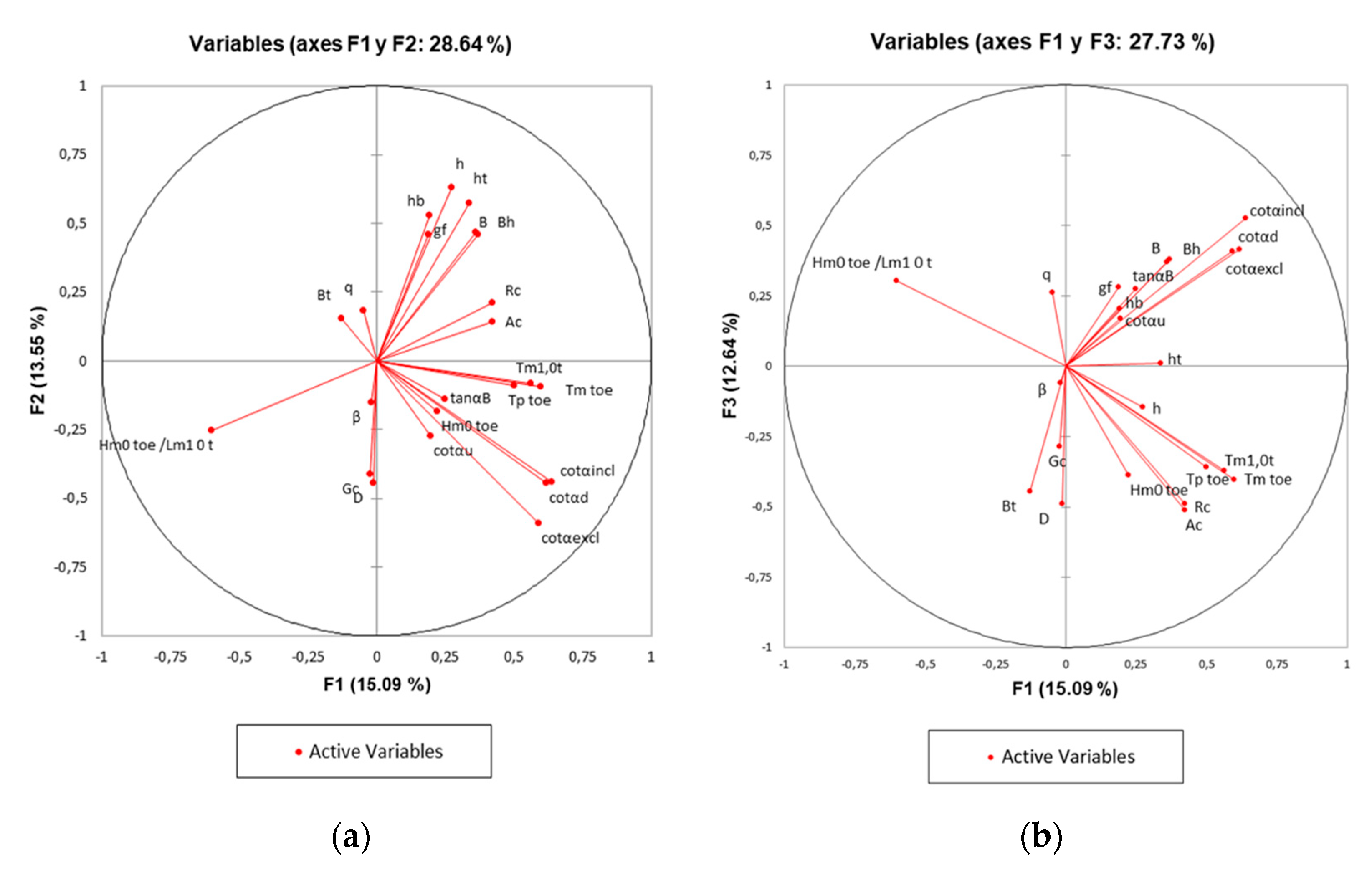
The first component (F1) explains 15.09% of the variance and is dominated by variables related with the period, slope of the structure and by the wave steepness. The second component (F2) with a similar percentage of the variance explained (13.55%) is dominated by variables related with the submergence and cotα_excl. And the third component (F3) explains 12.64% of the total variance and is dominated by the variables cotα_incl and A_c.

The analysis of the correlation circle, that corresponds to a projection of the initial variables of the first two factors of the PCA onto a two-dimensional plane, provides relevant information that allows observing correlations between the variables and interpreting the axes, or main factors, and thus being able to eliminate correlations that could be redundant and therefore detrimental to the predictability of the model. For the present case, it is shown, in the correlation circle (in the projection of both F1 and F2 axes) (See Figure 3a), that the percentage of variability represented by the first two factors is not particularly high (28.64%). Therefore, to avoid a misinterpretation of the graphics, it also requires a visualization in axes 1 and 3, and interpretation of the influence of presence or absence of certain parameters (See Figure 3b).

Both plots confirm the results shown in Table 4, without a significant relevance of the variables, accompanied by a lack of clear interpretation of the axes, but on the other hand, with the evidence of certain interesting relationships between the variables.

It can be seen that there is a strong grouping between the variables related to the period (T_m1.0t; T_{p t}; T_{m t}), with a high positive correlation between them, a trivial matter already detected in the correlation matrix, which at least allows reducing their number, in any case keeping only one of them. Another group with a strong positive correlation is composed of those variables related to the geometric characterization of the slope (cotα_incl; cotα_excl; cotα_d) on which it will act in a similar way. The same procedure can be carried out with the variables relative to the width of the berm and its horizontal projection (B; B_h), and from which it is inferred that only variable B will be preserved. The grouping of variables in the correlation circle, in the projection of both axes F1 and F2, seems to determine the lack of correlation between the variables that make up the most obvious groupings, with similar direct cosines, such as those determined by cotα_incl, cotα_excl, cotαd, and those like: cotα_u, tanα_B, H_{m0 t}. The foregoing leads to considering that both groupings of variables must be present in the input space, although with the particular restrictions indicated previously for some of them. The spectral wave steepness variable (H_{m0 t}/L_{m1 t}), negatively correlated with the freeboard variables (R_c, A_c), should be kept as above. Finally, the strong link between the width of the crest and the characteristic size of the protection elements in the breakwater is clearly reflected along with its strong link with the F2 axis.

The projection on the F1 and F3 axes explain a total variability of 27.7%, which is a percentage very similar to that explained by the previous projection (F1 and F2). Additionally, in this projection the correlations established for the first circle of projections are maintained, even the observed groupings are very similar. This robustness in the projection reaffirms the initial idea of finally discarding several of these correlated variables.

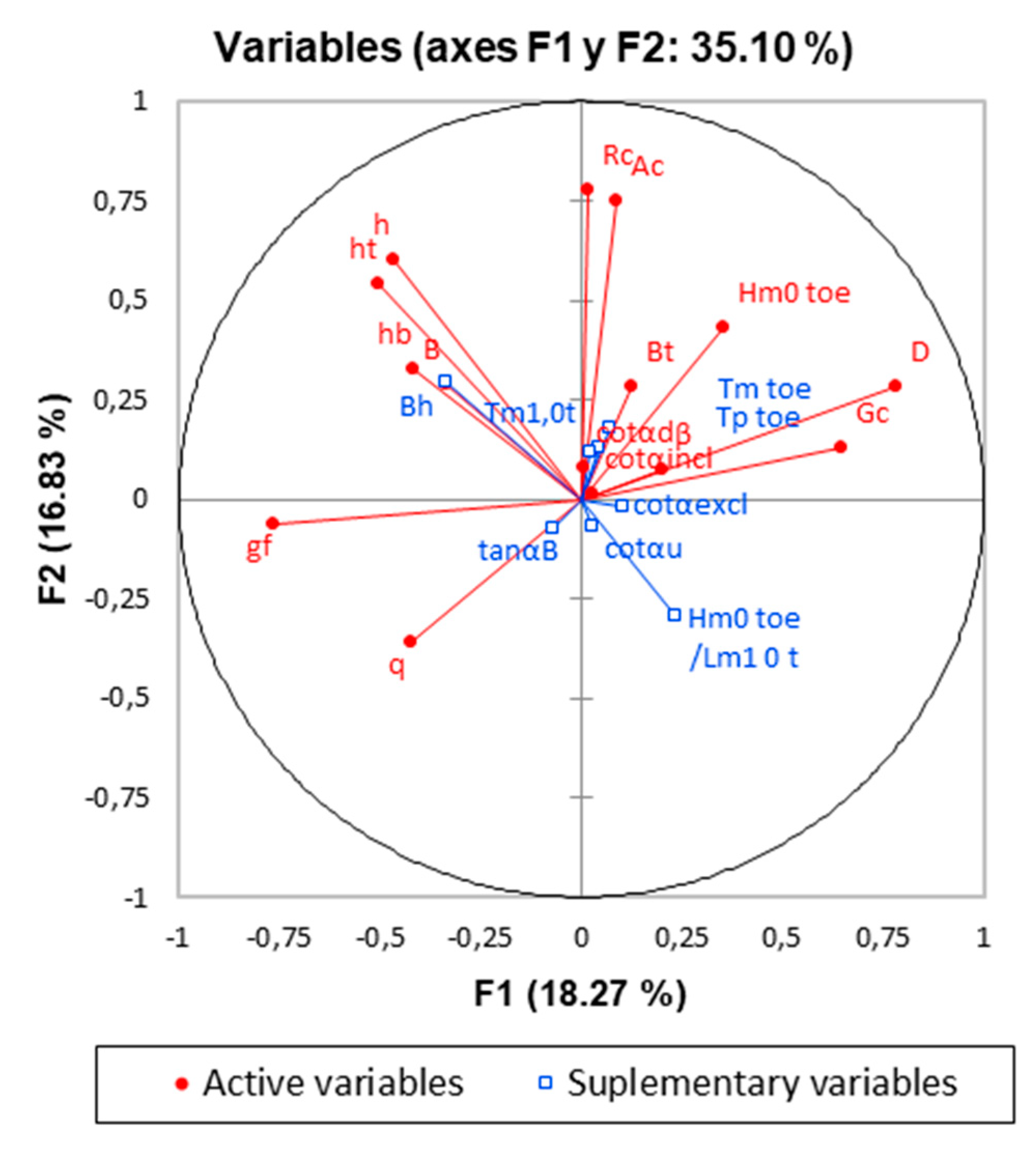
A technique that is usually used when the information provided by the PCA analysis carried out on the total of the variables is not very informative, is to consider the contribution of some variables whose contribution is doubted, such as that of supplementary variables studying the effect of their elimination on the projection space. In this case, the input space is censored by considering as supplementary variables all those that have shown an evident correlation in the previous projections. Figure 4 shows the new correlation circle with this elimination step applied.

Figure 4 demonstrates that the variability explained by the first two factors increases slightly with a total of the variance explained equal to 35.10%. Additionally, that there is strong linking between variables relates with freeboard parameters and F1 axis, which could explain the major variance in the sample. The above, and its comparison with the initial projections, indicates that a reduction in dimensionality may be beneficial for the explanation of the problem without a significant loss of information [53], and therefore this reasoning can be valid for the composition of a model with a smaller input dimension.

Alternatively, the application of a Kohonen network model on the same input pattern space, with a dimension of 23 factors (all of which come from the previous pre-processing processes), will indirectly allow the interpretation of the relationships existing at the level of self-similarity between input patterns, in a two-dimensional projection, where every pixel in that 2-dimensional map is characterized by a multidimensional vector. Information that will ultimately allow the reduction of the dimensionality of the entrance space, either by interpretation of these detected relationships, or by confirmation of those already detected using the PCA technique.

For the specific purposes of the present study, the constructed model, built with a Gaussian neighborhood function in every node, has been carried out using the following training scheme, characterized by two different phases [66], where each set is shown 500 times to the SOM. During the training phase, the complete preprocessed data set is shown 500 times to the SOM, built with a Gaussian neighborhood function in every node. The first of these, or rough adjustment phase, is performed with a learning rate with values in the range between 0.9 to 0.1, and with a neighborhood ratio that varies from 2 to 1, and with an extension of training up to 100 times. The second or fine-tuning phase is completed with a unique learning rate of η = 0.01, with a neighborhood ratio of 0, and with training extension up to 100 epochs. With this, the total length of the training will be: 100 + 100 = 200 times. The dimension of the input tile for this model will be 25 × 25 units (625 total units).

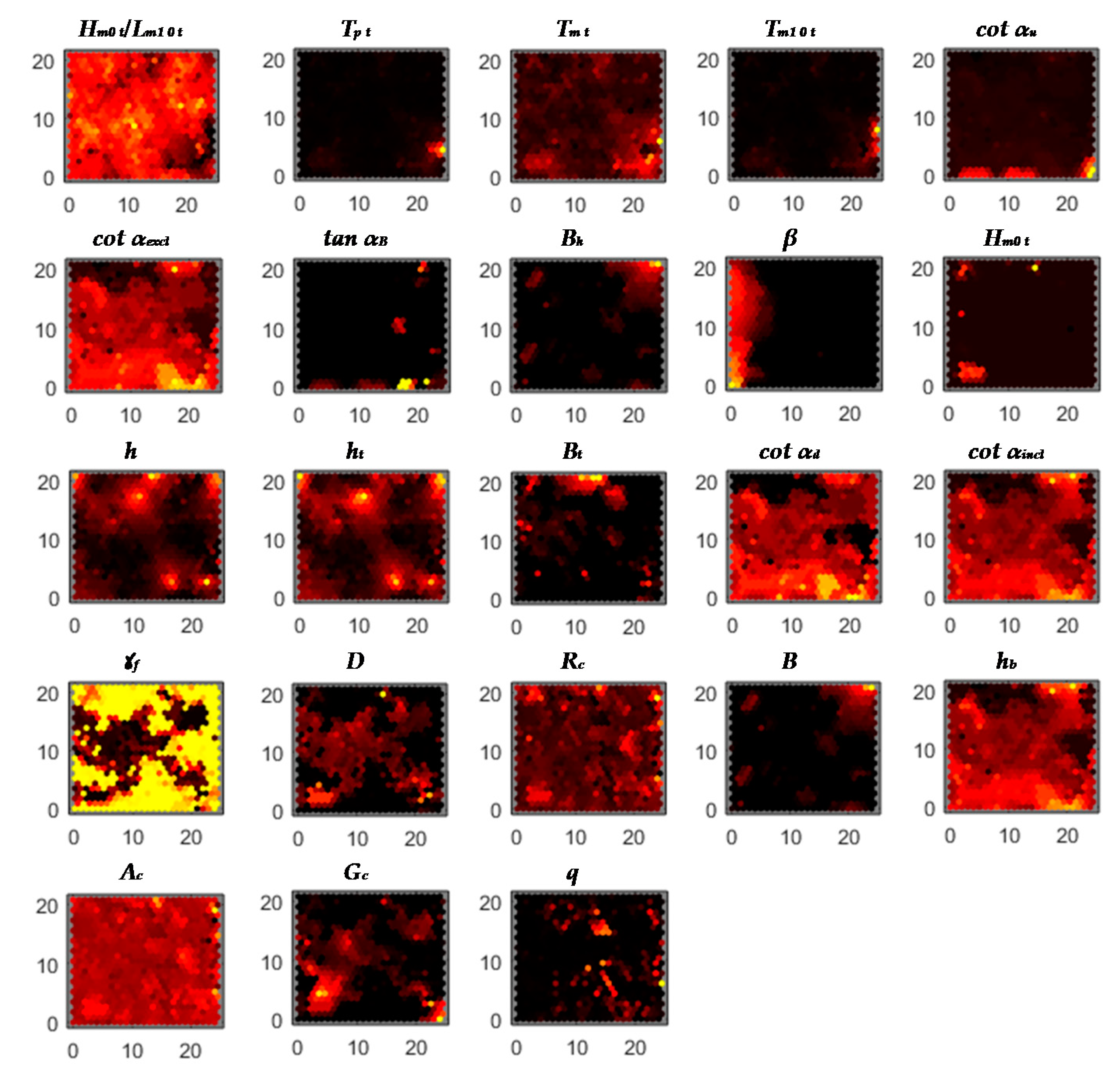
The following figure (Figure 5) shows the different component planes obtained after network training, with a total of 23 units (one for each component variable of the input and output space).

From the analysis of these component planes the existence of several evident relationships between the variables is deduced. The first of these concerns the parameters related to the definition of the slopes of the dykes and which comparatively shows the existence of a direct and significant correlation across the entire range of the data between the variables (cotα_excl, cotα_incl, cotα_d). A reason why the information contributed by them can be redundant, and informs which two of them should be discarded. However, it is noteworthy that another of the variables related to that group of parameters, which refers to the cotangent of the slope of the structure in the part of the slope above the berm (cotα_u), presents a projection pattern that is notoriously different from the previous ones, but without a distinctive response in the component plane, so it should not be taken into account.

Another very significant relationship detected by the SOM is the one that shows the component planes of the roughness factor variables (γ_f) and the mean diameter (D). The comparison of both planes shows the existence of a negative correlation between them, and thus the greater sizes, the lower the roughness factor. This relationship is evidence in the existing empirical knowledge and taken into account [32,41], but it is comforting to confirm that the ANN is capable of detecting it as well. Both parameters should be preserved a priori.

The next detected relationship is the one between the width of the berm (B) and its projected width (B_h), and that is also preserved across the data range. Therefore, only one of them should be selected, discarding the other.

It could be thought that, based on design criteria, there was a direct relationship between the width of the berm and the width of the toe (B_t), or with the width of the crest, however, this has not been detected at the data base analyzed for the crest width of the structure, so this supposed relationship will be discarded. While the existence of a partial correlation, at least in a region of the projection plane, between the variables of the berm width and the width of the bench (see Figure 5) is detected, which indicates that some of the breakwaters that have been tested have been designed with a theoretical pattern that relates both variables. The foregoing forces not discarding these variables, but to keep them in the input space, since this relationship is partial in the sample space it is necessary to preserve that differentiation.

A last relationship highlighted (Figure 5), and also expected by the existing empirical knowledge, is the one presented by the depth variables at the toe of the structure (h), and the one that define the submergence of it (h_t). In this case, as expected, its correlation is direct or positive. However, the lack of correlation between both variables and the berm (h_b) is also striking, therefore, following the above reasoning, at least two of them should be maintained, discarding the third of them.

In view of the results obtained and interpreted after applying both the PCA technique and the SOM maps, a reduction in the size of the input patterns can be achieved. It results in a final dimension of the input vector of 15 parameters (see

Table 5. Selected variables that finally composes the input vector for the ANN modelling.

Parameter 1	Description	Unit
Hm0 toe/Lm−1	Dimensionless spectral wave steepness	-
β	Wave incidence angle	◦
Tm t	Average period at the toe of the structure	s
Hm0 toe	Significant spectral wave height at the foot of the structure	m
h	Water depth at the structure toe	m
ht	Toe submergence	m
Bt	Toe width	m
cotαincl	Average co-tangent of the slope of the structure, considering the contribution of the berm	-
γf	Roughness/permeability factor for the structure	-
B	Berm width	m
D	Size of the structure elements along the slope	m
hb	Berm submergence	m
Rc	Crest freeboard of the structure respect to sea water level (swl)	m
Ac	Armour crest freeboard respect to swl	m
Gc	Crest width	m

¹ Windward side.

).

3.2. Model Selection

The results obtained after the training process of the different architectures tested for each model, show better performance of the aggregate model (Model I) over the disaggregated model (Model II), both in terms of error and correlation, as shown in

Table 6. Model I: Results in the test subset based on the number of neurons in the hidden layer. MSE and r statistic.

N° ud.	5	10	15	20	25	30	35
MSE	7.02 × 10−5	6.75 × 10−5	5.69 × 10−5	5.72 × 10−5	3.82 × 10−5	5.06 × 10−5	7.08 × 10−5
r	96.51	96.28	97.33	97.17	98.17	97.68	97.28

,

Table 7. Model II.I: Results in the test subset based on the number of neurons in the hidden layer. MSE and r statistic.

N° ud.	5	10	15	20	25	30	35
MSE	7.02 × 10−5	6.71 × 10−5	8.43 × 10−5	5.86 × 10−5	3.82 × 10−5	6.28 × 10−5	6.98 × 10−5
r	96.98	96.24	96.31	97.37	96.13	97.28	96.81

and

Table 8. Model II.II: Results in the test subset based on the number of neurons in the hidden layer. MSE and r statistic.

N° ud.	5	10	15	20	25	30	35
MSE	1.68 × 10−7	1.82 × 10−7	3.00 × 10−7	3.88 × 10−8	1.45 × 10−8	1.46 × 10−7	1.02 × 10−7
r	84.05	63.10	66.10	84.51	75.33	74.66	74.52

, and Figure 6, in which is possible to distinguish the results for each of the subsets used in the cross-verification process: Training (TR), Verification (V), Test (T) of the better Model I.

The finally selected architecture for Model I, based on the results obtained, is an MLP network with 15 input variables, 25 neurons in the hidden layer, and a single neuron in the output layer (see Table 6, Table 7 and Table 8, with the trial results to determine the best architecture in the results of the different models proposed).

The results are shown in the form of correlation plots for test subset in Figure 6. Noting that for the test subset the correlation values are greater than 0.98. Although they are similar to those obtained for sub model II.1 (0.96), they are much higher than those obtained with sub model II.2 (0.84). The results in terms of error (MSE) are similar for both model I (3.85 × 10⁻⁵) and model II (3.82 × 10⁻⁵), with the known exception that the MSE is not an absolute statistic, but a relative one [64].

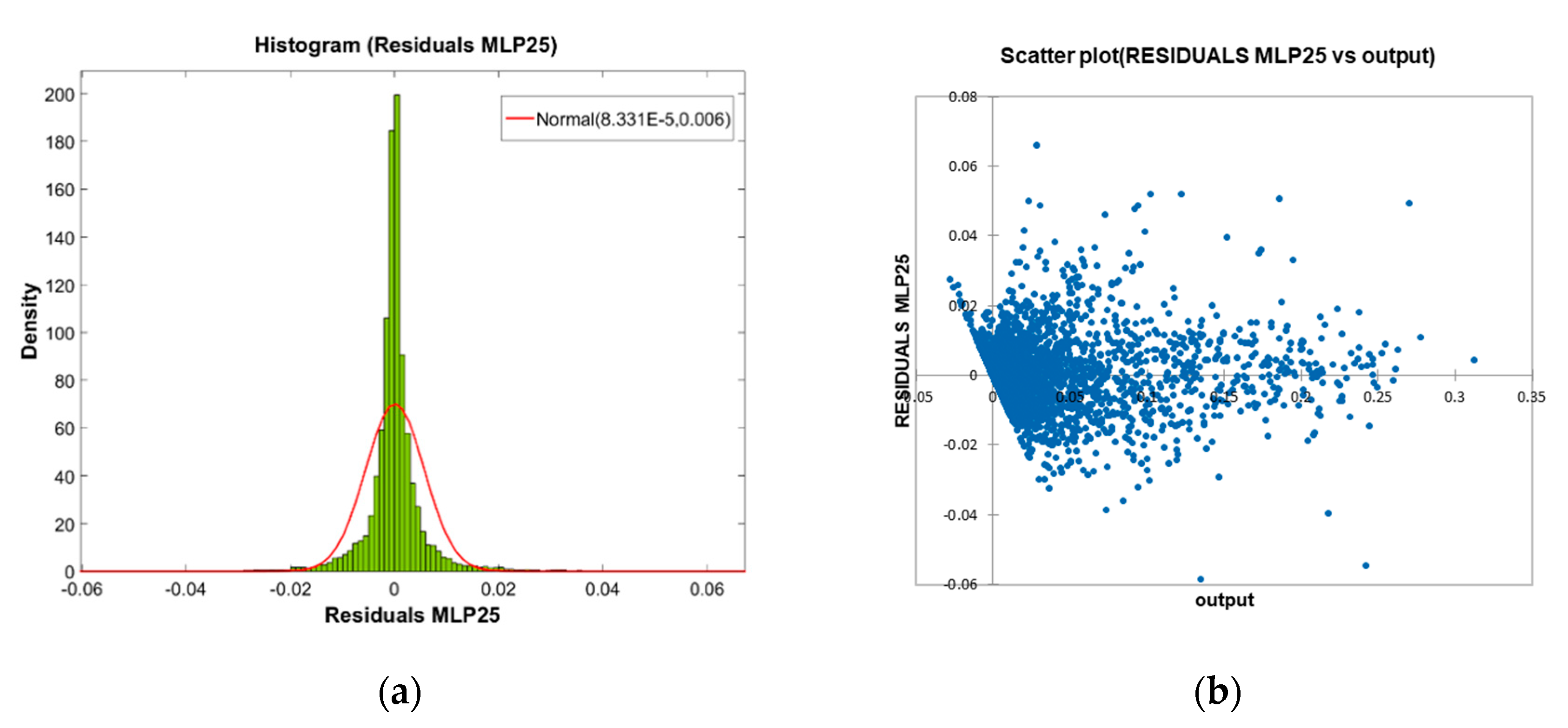
The analysis of the residuals establishes, as a desirable objective for an ideal model, that its distribution be carried out according to a pattern as close as possible to a normal distribution as a clear indicator of the absence of any hidden trend or bias in the modelling performed. In the present case, a careful analysis of this distribution shows that although it is close to normal, it does not fit significantly to it. This is demonstrated by the chi-square and Kolmogorov-Smirnov fit tests carried out, and that they are presented below (see

Table 9. Results of the different contrast test on the residuals for the selected model.

Statistics	Chi-Squared	Kolmogorov-Smirnov
Empirical Parameter	3.922 × 1015	0.161
Theoretical Parameter	72.15
p-value (bilateral)	<0.0001	<0.0001
Confidence interval (α)	0.05	0.05

), together with their correspondent graphical adjustment (Figure 7a).

The graphical analysis of the scatter plot of the residuals (Figure 7b) shows adequate behavior across the entire response range, except in the range of low values of overtopping rate, for which it does show a certain tendency towards non-compliance with the hypothesis of constant variance of the residuals. This heteroscedasticity may be linked to scale problems in the tests or introduced by iso-energetic sequences of waves [60,61], since the behavior of the prediction for very low overtopping rates has been associated with high levels of uncertainty [69], or may be due to the need to perform further specific transformations on the input variables beyond those already applied in the present study [25].

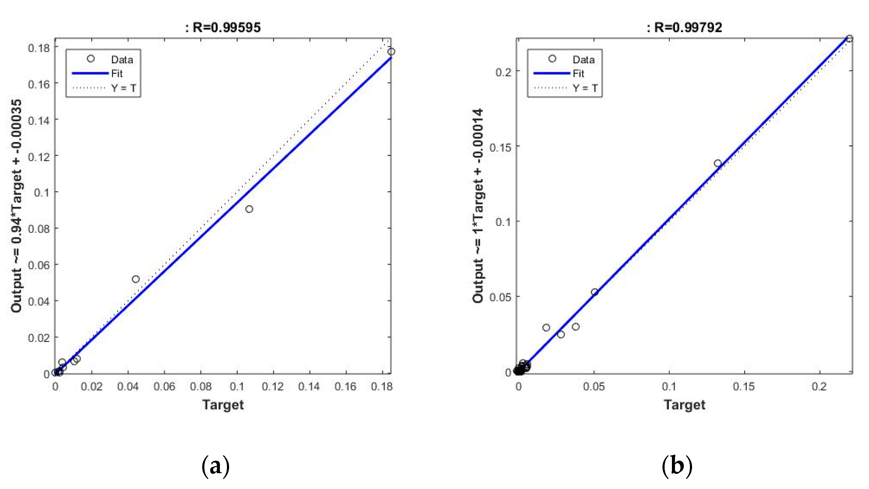
An extra validation test performed on an additional sample of 100 patterns, and with the selected ANN, provides good performance, with correlations of 0.98, which could validate its generalizability. However, what is more interesting, after classifying the component patterns into two different classes, the first one corresponding to tests on seawalls, and the second corresponding to sloped breakwaters, they show a similar aspect and is very suitable for the prediction of the overtopping rate on both (see Figure 8). Thus, the results for the typology of seawalls provides a correlation coefficient of 0.996, while for slope breakwaters it provides a similar result of 0.998.

3.3. Sensitivity Analysis

Finally, a sensitivity analysis is carried out on the selected ANN, specifically on the component parameters of the input vector. This analysis is performed using a pruning technique, and the ratio that was proposed for this purpose:

$$r_s=\frac{e{r}_j}{e{r}_T}$$

(12)

where ${\mathrm{x}}^{\prime }$ is the sensibility ratio, and $e{r}_j$ the error function value for the trained network. In this case, the MSE is chosen as the error criterion to define the sensitivity ratio.

This procedure is especially useful when the input variables are essentially independent of each other [64], and conversely, the more interdependencies there are between the variables, the less reliable they will be. Hence, among other reasons, the importance of the previously performed dimensionality reduction procedure, which now supports the application of that sensitivity analysis.

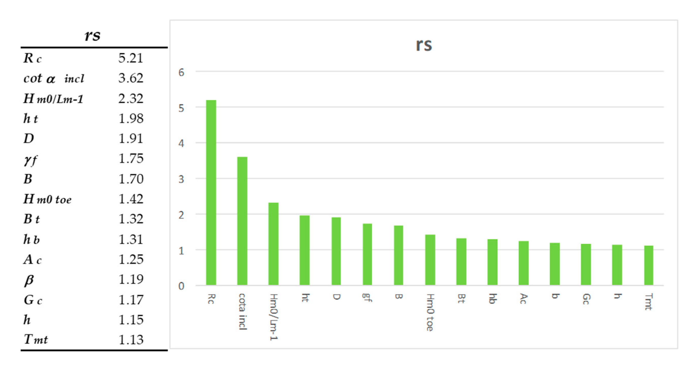
It is observed in the Figure 9 that all the variables have a significance ratio greater than 1.05, which according to that criterion implies that all the variables are significant a priori, and that therefore it would be desirable to maintain them for adequate network performance. The above has a clear derivative, which is to suppose that the process of dimensionality reduction has been successful, since any of the existing variables will provide enough relevant information and their elimination may imply worse predictive capacity of the network.

Beyond the previous observations, it is noted that the most influential variable is the freeboard of the wall with respect to swl (R_c), an issue that is confirmed by PCA analysis. It is noteworthy that a variable closely related to it, the other freeboard parameter, the crest height with respect to swl (A_c), is quite far, in terms of significance, from the parameter R_c. This fact is relevant since in some works [59] it has been determined that the scale effect seems to depend a lot on the superior geometry of the breakwater. This results in many more significant associated effects on small overtopping rates, which are incidentally, also the most numerous in the database. Given this, and to try to mitigate these effects as much as possible, some authors propose the dimensionless of these variables [25,30,59].

Another significantly interesting variable is the average cotangent where the contribution of the berm (cotα_incl) is considered [42,59]. Similarly of interest, the wave steepness (H_m0/L_m−1) is highlighted. In addition to these, are both parameters related to roughness (and in essence, to the porosity of the mantle) where their close relationship with overtopping is already known empirically [32], and which in turn have a substantial dependence on the dimensionless freeboard (R_c/H_m0).

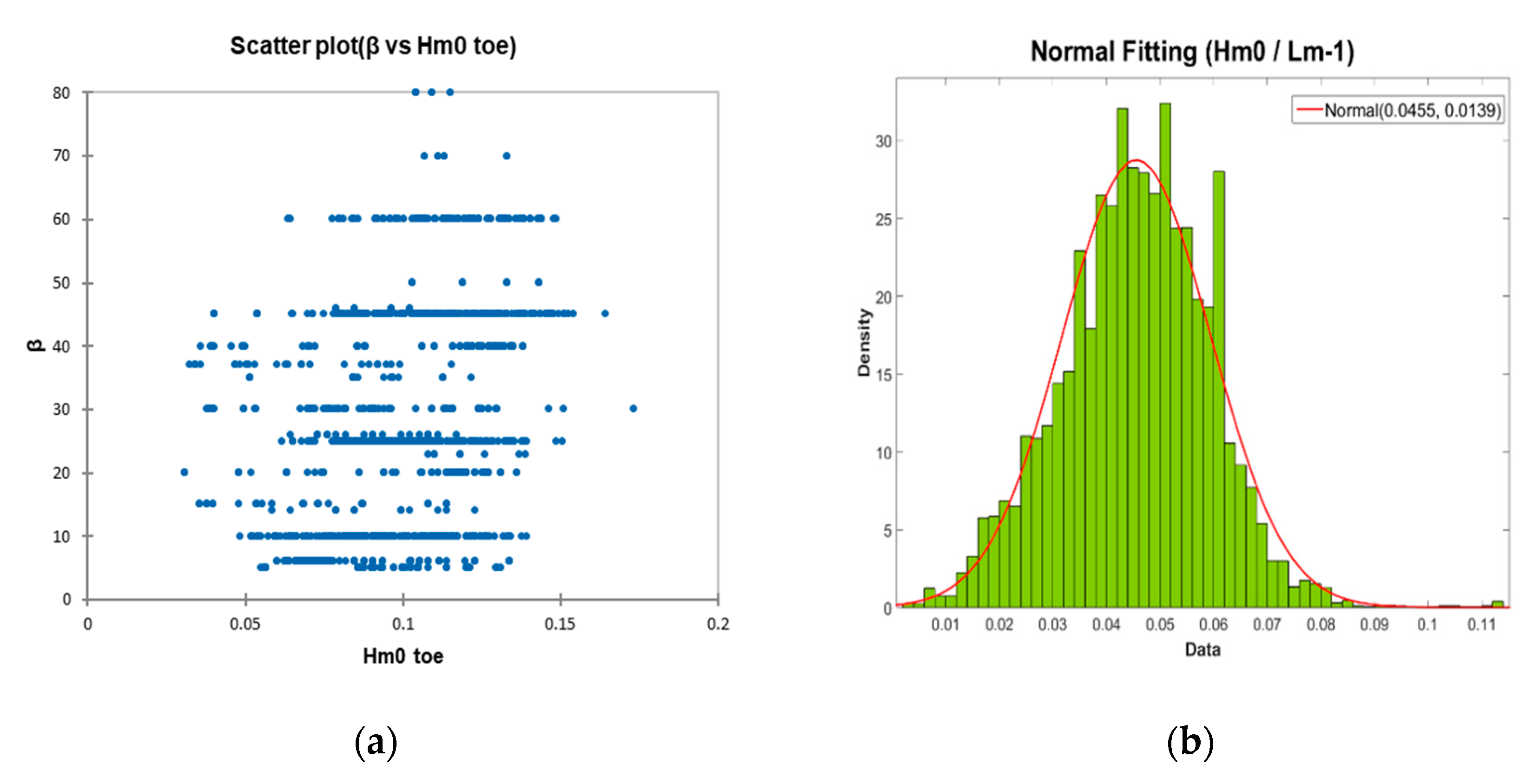
Overall, the results are consistent in terms of the significance of these parameters with similar studies carried out with different preprocessing techniques [30]. And it should be mentioned that some parameters in this study are may be penalized, due to the fact that they have been poorly represented in the database. For example, this happens with the wave incidence angle parameter (β) that shows a significant lack of data in some ranges of that continuous variable. In the following figure (see Figure 10a) the distribution of the aforementioned parameter with respect to the significant wave height at the toe structure (H_{mo t}) is presented since, as Van der Meer cites [48], this relationship is strongly related to the overtopping phenomenon, and shows the existence of poor representability in the ranges greater than 50°.

The importance given to the dimensionless parameter of the wave steepness, particularly for wave overtopping energy conversion [70], which has good representation in the database, both in its distribution and in the quality of that distribution (normalized distribution), should also be highlighted (see Figure 10b). Faced with possible uncertainties associated with scale phenomena [59], although the parameter’s existence in the field of validity is remarkable with values over 0.07 that are physically not possible as the wave breaks on steepness [56], the use of wave steepness as a variable is recommended. This also represents the effects induced by local breakage and waves [25], and is therefore strongly related with the overtopping.

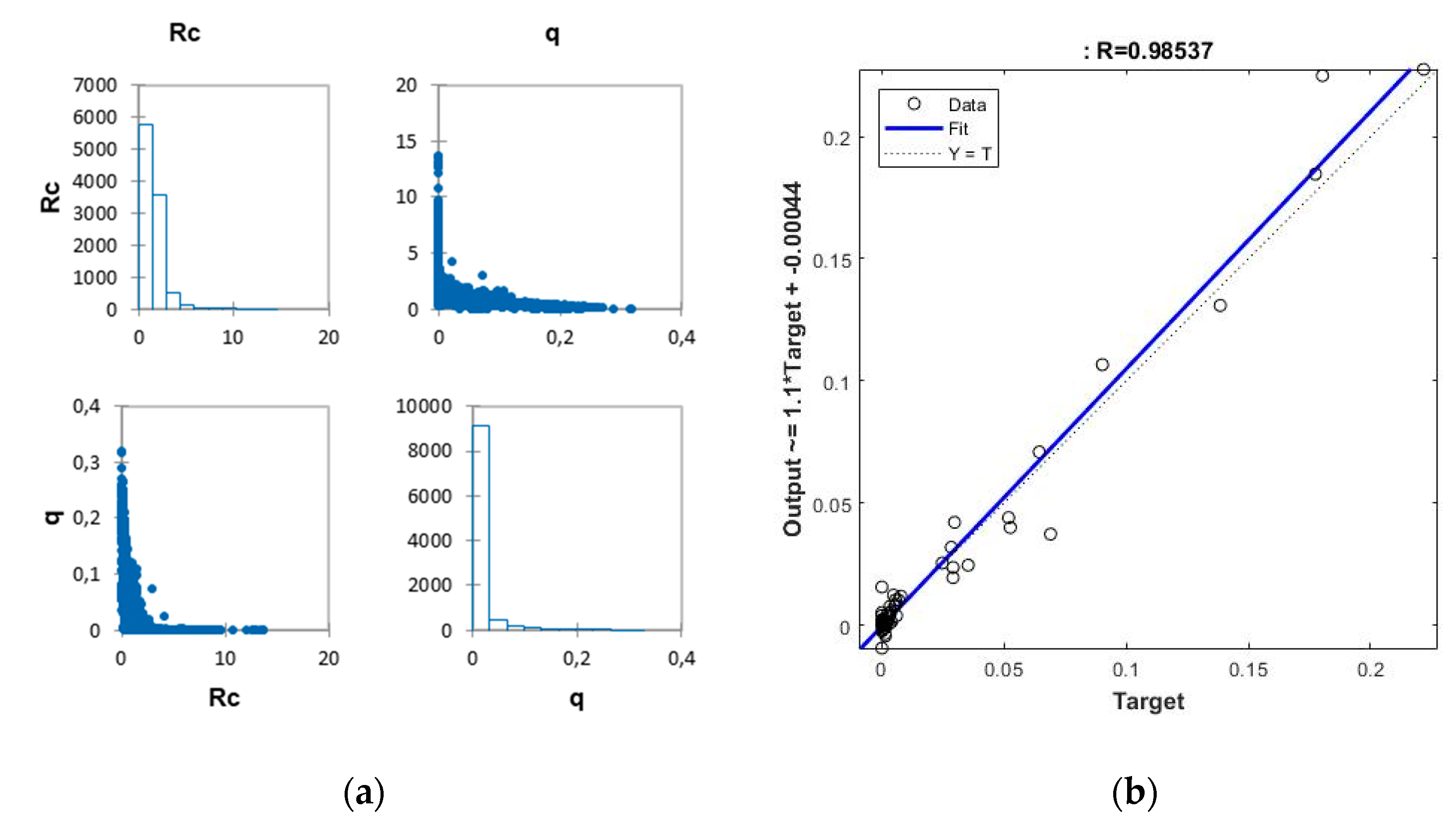
Due to the fact that for wave overtopping conversion the maximum overtopping rates correlated with the lower R_c/H_s relationships [71] are highly desirable. These will generally be associated with low crested structures, specifically with R_c/H_s lower than 1. It would be desirable that the training sample be well represented in this range, as does happen, and is shown in the following figure (Figure 11a). Checking the model for those exceedance rates corresponding to the range in the previously mentioned sample of 100 extra cases (corresponding to a total of 57 cases), the result is encouraging, with values of the correlation coefficient greater than 0.98, as shown in the Figure 11b.

Thus, and in accordance with the above mentioned, any future improvement in the model should necessarily focus on that data range. This desired approach is in practice the opposite of what is usually done for defense structures.

Another crucial issue related to the generation of the data is the need to make the range of data tested wide enough to include extraordinary events, given that ANNs are usually unable to extrapolate beyond the range of the data used for training [65,72]. This ensures that they always work in the expected range, avoiding poor predictions when the validation data contain values outside of the range of those used for training. In this sense, there is a preponderance of low flow rates that reinforces the idea of a disaggregated approach in future models.

4. Conclusions

As part of a sustainable strategy to take advantage of some existing breakwater infrastructure, and its partial reconversion as a Wave Energy Converter while maintaining its defense purpose, this study is framed in which a model based on artificial neural networks for the overtopping rate forecasting is proposed for a wide range of breakwaters. The adjusted prediction of the overtopping rate constitutes the first step in the study of subsequent modifications to be made to these structures.

To achieve this purpose, existing data from CLASH-EurOtop have been subjected to a preprocessing step, where only the parameters from laboratory tests have been previously scaled according to the Froude model law (to H_{m0 toe} = 1 m). Subsequently, the entire data base was subjected to an extensive process of exploration, debugging, and dimensionality reduction, until an optimized input pattern in the ANN model was obtained. Using only 15 of the 34 initial features, sufficient relevant information was used to train a model with generalization skills and high predictive efficiency. This preliminary phase derives substantial conclusions such as:

• It is worth noting the lack of homogeneity in the database due to its diverse origin, where the existence of data at different scales forces the adoption of a data scaling procedure, which introduces uncertainty into the model. It is concluded that this lack of homogeneity is masked in the final model by the significant difference in sample size.
• Relevant effects associated to the scale are quoted, especially in what concerns to the superior geometry of the breakwater. WEC devices that are located in existing structures, where power generation capacity is combined with defensive capacity, that have small magnitudes of the overtopping rate, and which incidentally are the most common, are especially sensitive to these effects.
• Linked with the above conclusion, a new and more appropriate transformation of the inputs must be proposed that minimizes the observed heteroscedasticity effects in this range of overtopping rates.
• The present work shows the suitability of multivariate statistical techniques, and specifically the Mahalanobis distance, for the detection of outliers, and also the Principal Component Analysis for the reduction of the dimension of the input vector, a task shared with the Kohonen Self Organizing Maps application.

Several ANN models have been proposed and the architecture finally selected has been an MLP 15-25-1. This was obtained after a cross-verification training process with the Levenberg-Marquardt algorithm, and which corresponds to a model that takes into account both the data from prototypes and small-scale tests.

The results are very encouraging since they allow obtaining predictions with very high correlation coefficients (>0.98) and where the validation process carried out shows that the model is equally suitable for both seawalls and slope breakwaters. This has been justified by the prevalence of those that refer to crest freeboard of the structure with respect to swl over the rest of the parameters, and the average cotangent of the slope of the structure considering the contribution of the berm.

This final conclusion reinforces the belief that subsequent studies, in which an adequate classification criterion of the input parameters will be obtained, will undoubtedly reinforce the good performance of the ANN model. For wave energy conversion, the lower R_c/H_s relationship the higher overtopping rate, therefore this criterion will allow future models to be developed and trained in that specific range of patterns.

References

1. IEA-OES (International Energy Agency-Ocean Energy Systems). Annual Report 2006; Technical Report; IEA-OES: Paris, France, 2006. [Google Scholar]
2. Esteban, M.D.; Espada, J.M.; Ortega, J.M.; López-Gutiérrez, J.S.; Negro, V. What about Marine Renewable Energies in Spain? J. Mar. Sci. Eng. 2019, 7, 249. [Google Scholar] [CrossRef] [Green Version]
3. Breeze, P. Marine Power Generation Technologies. In Power Generation Technologies, 3rd ed.; Elsevier Ltd.: Oxford, UK, 2019; pp. 323–349. [Google Scholar]
4. Zhou, Z.; Benbouzid, M.; Charpentier, J.F.; Scuiller, F.; Tang, T. A Review of Energy Storage Technologies for Marine Current Energy Systems. Renew. Sustain. Energy Rev. 2013, 18, 390–400. [Google Scholar] [CrossRef] [Green Version]
5. Lewis, M.; Neill, S.; Robins, P.; Hashemi, M. Resource assessment for future generations of tidal-stream energy arrays. Energy 2015, 83, 403–415. [Google Scholar] [CrossRef] [Green Version]
6. Lavi, A. Ocean thermal energy conversion: A general introduction. Energy 1980, 5, 469–480. [Google Scholar] [CrossRef]
7. Seyfried, C.; Palko, H.; Dubbs, L. Potential local environmental impacts of salinity gradient energy: A review. Renew. Sustain. Energy Rev. 2019, 102, 111–120. [Google Scholar] [CrossRef]
8. Falcão, A.F.O. Wave energy utilization: A review of the technologies. Renew. Energy 2010, 14, 899–918. [Google Scholar] [CrossRef]
9. Babarit, A.; Bull, D.; Dykes, K.; Malins, R.; Nielsen, K.; Costello, R.; Roberts, J.; Bittencourt Ferreira, C.; Kennedy, B.; Weber, J. Stakeholder requirements for commercially successful wave energy converter farms. Renew. Energy 2017, 113, 742–755. [Google Scholar] [CrossRef]
10. IDAE. Evaluación del Potencial de la Energía de las olas; Technical Report; IDEA: Madrid, Spain, 2011. [Google Scholar]
11. Margheritini, L.; Vicinanza, D.; Frigaard, P. SSG wave energy converter: Design, reliability and hydraulic performance of an innovative overtopping device. Renew. Energy 2009, 34, 1371–1380. [Google Scholar] [CrossRef]
12. Astariz, S.; Iglesias, G. The economics of wave energy: A review. Renew. Sustain. Energy Rev. 2015, 45, 397–408. [Google Scholar] [CrossRef]
13. Reguero, B.G.; Losada, I.J.; Méndez, F.J. A global wave power resource and it seasonal, interannual and long-term variability. Appl. Energy 2015, 148, 366–380. [Google Scholar] [CrossRef]
14. Shields, M.A.; Payne, A.I.L. Strategic Sectoral Planning for Offshore Renewable Energy in Scotland. In Marine Renewable Energy Technology and Environmental Interactions, 1st ed.; Shields, M.A., Payne, A.I.L., Eds.; Springer: Berlin, Germany, 2014; pp. 141–152. [Google Scholar]
15. Aderinto, T.; Li, H. Ocean Wave Energy Converters: Status and challenges. Energies 2018, 11, 1250. [Google Scholar] [CrossRef] [Green Version]
16. The Wave Dragon Technology. Wave Dragon Web Site. Available online: http://www.wavedragon.net/?option=com_content&task=view&id=4&Itemid=35 (accessed on 1 June 2020).
17. Foteinis, S.; Tsoutsos, T. Strategies to improve sustainability and offset the initial high capital expenditure of wave energy converters (WECs). Renew. Sustain. Energy Rev. 2017, 70, 775–785. [Google Scholar] [CrossRef]
18. Contestabile, P.; Iuppa, C.; Di Lauro, E.; Cavallaro, L.; Andersen, T.L.; Vicinanza, D. Wave loadings acting on innovative rubble mound breakwater for overtopping wave energy conversion. Coast. Eng. 2017, 122, 60–74. [Google Scholar] [CrossRef]
19. Iuppa, C.; Contestabile, P.; Cavallaro, L.; Foti, E.; Vicinanza, D. Hydraulic Performance of an Innovative Breakwater for Overtopping Wave Energy Conversion. Sustainnabily 2016, 8, 1226. [Google Scholar] [CrossRef] [Green Version]
20. Vicinanza, D.; Nørgaard, J.H.; Contestabile, P.; Andersen, T.L. Wave loadings acting on Overtopping Breakwater for Energy Conversion. J. Coast. Res. 2013, 65, 1669–1674. [Google Scholar] [CrossRef]
21. Cuadra, L.; Salcedo-Sanz, S.; Nieto-Borge, J.C.; Alexandre, E.; Rodríguez, G. Computational intelligence in wave energy: Comprehensive review and case study. Renew. Sustain. Energy Rev. 2016, 58, 1223–1246. [Google Scholar] [CrossRef]
22. Govindaraju, R.S.; Rao, A.R. Artificial Neural Networks in Hydrology, 1st ed.; Water Science and Technology Library, Kluwer Academic Publishers: Dordrecht, The Netherlands, 2000; pp. 1–329. [Google Scholar]
23. Bishop, C.M. Neural Networks. In Pattern Recognition and Machine Learning, 3rd ed.; Springer: New York, NY, USA, 2006; pp. 225–290. [Google Scholar]
24. Van Gent, M.R.A.; Van den Boogaard, H.F.P.; Pozueta, B.; Medina, J.R. Neural network modelling of wave overtopping at coastal structures. Coast. Eng. 2007, 54, 586–593. [Google Scholar] [CrossRef] [Green Version]
25. EurOtop Manual. EurOtop-Wave Overtopping of Sea Defenses and Related Structures. An Overtopping Manual Largely Based on European Research, but for Worldwide Application, 2nd ed. 2018. p. 320. Available online: https://www.overtopping-manual.com (accessed on 24 May 2020).
26. Formentin, S.M.; Zanuttigh, B. A methodological approach for the development and verification of artificial neural networks based on application to wave-structure interaction processes. Coast. Eng. J. 2018, 60, 1–20. [Google Scholar] [CrossRef]
27. Verhaeghe, H.; De Rouck, J.; Van der Meer, J.W. Combined classifier–quantifier model: A 2-phases neural model for prediction of wave overtopping at coastal structures. Coast. Eng. 2008, 55, 357–374. [Google Scholar] [CrossRef]
28. Peixó, J.; Van Oosten, R.P. Wave Transmission at Various Types of Low-Crested Structures Using Neural Networks. Master’s Thesis, Delft University of Technology, Delft, The Netherlands, 2005. [Google Scholar]
29. Panizzo, A.; Briganti, R. Analysis of wave transmission behind low-crested breakwaters using neural networks. Coast. Eng. 2007, 54, 643–656. [Google Scholar] [CrossRef]
30. Formentin, S.M.; Zanuttigh, B.; Van der Meer, J.W.A. Neural Network Tool for Predicting Wave Reflection, Overtopping and Transmission. Coast. Eng. 2017, 59, 1–31. [Google Scholar] [CrossRef]
31. Zanuttigh, B.; Formentin, S.M.; Briganti, R. A neural network for the prediction of wave reflection from coastal and harbour structures. Coast. Eng. 2013, 80, 49–67. [Google Scholar] [CrossRef]
32. Molines, J.; Medina, J.R. Explicit Wave-Overtopping Formula for Mound Breakwaters with Crown Walls Using CLASH Neural Network–Derived Data. J. Waterw. Port Coast. Ocean Eng. 2016, 142, 1–13. [Google Scholar] [CrossRef] [Green Version]
33. Deo, M.C. Artificial neural networks in coastal and ocean engineering. Indian J. Geo-Mar. Sci. 2010, 34, 589–596. [Google Scholar]
34. Najafzadeh, M.; Barani, G.A.; Hessami-Kermani, M.R. Group method of data handling to predict scour depth around vertical piles under regular waves. Sci. Iran. 2013, 20, 406–413. [Google Scholar]
35. Azamathulla, H.M.; Zakaria, N.A. Prediction of scour below submerged pipeline crossing a river using ANN. Water Sci. Technol. 2011, 63, 2225–2230. [Google Scholar] [CrossRef]
36. Ayoubloo, M.K.; Etemad-Shahidi, A.; Mahjoobi, J. Evaluation of regular wave scour around a circular pile using data mining approaches. Appl. Ocean Res. 2010, 32, 34–39. [Google Scholar] [CrossRef] [Green Version]
37. Bateni, S.M.; Borghei, S.M.; Jeng, D.S. Neural network and neuro-fuzzy assessments for scour depth around bridge piers. Eng. Appl. Artif. Intell. 2007, 20, 401–414. [Google Scholar] [CrossRef]
38. López, I.; Aragonés, L.; Villacampa, Y.; Satorre, R. Modelling the cross-shore beach profiles of sandy beaches with Posidonia oceanica using artificial neural networks: Murcia (Spain) as study case. Appl. Ocean Res. 2018, 74, 205–216. [Google Scholar] [CrossRef]
39. Negro, V.; Varela, O. Comportamiento funcional, reflexión, transmisión, y amortiguación. Remonte, descenso y rebase. In Diseño de Diques Rompeolas, 2nd ed.; Colegio de Ingenieros de Caminos Canales y Puertos: Madrid, Spain, 2010; pp. 267–304. [Google Scholar]
40. Rodríguez, A.M.; Sánchez, J.F.; Gutiérrez, R.; Negro, V. Overtopping of harbour breakwaters: A comparison of semi-empirical equations, neural networks, and physical model tests. J. Hydraul. Res. 2015, 53, 1–14. [Google Scholar] [CrossRef] [Green Version]
41. Verhaeghe, H.; Van der Mer, J.W.; Steendam, G.J.; Besley, P.; Franco, L.; Van Gent, M.R.A. Wave overtopping database as the starting point for a neural network prediction method. In Coastal Structures; ASCE: Portland, OR, USA, 2003; pp. 418–429. [Google Scholar]
42. De Rouck, J.; Geeraerts, J. CLASH—D46: Final Report; Full Scientific and Technical Report; Gent University: Gent, Belgium, 2005. [Google Scholar]
43. Haykin, S. Neural Networks: A Comprehensive Foundation, 2nd ed.; Pearson Prentice Hall: Upper Saddle River, NJ, USA, 1999; pp. 1–823. [Google Scholar]
44. Kohonen, T. Self-Organized Formation of Topologically Correct Feature Maps. Biol. Cybern. 1982, 43, 59–69. [Google Scholar] [CrossRef]
45. Kohonen, T. Self-Organizing Map, 3rd ed.; Springer: New York, NY, USA, 2001; pp. 1–501. [Google Scholar]
46. Van der Meer, J.W.; Van Gent, M.R.A.; Pozueta, B.; Steendam, G.J.; Medina, J.R. Applications of a neural network to predict wave overtopping at coastal structures. In Proceedings of the International Conference on Coastlines, Structures and Breakwaters, London, UK, 20–22 April 2005; ICE Thomas Telford: London, UK, 2005; pp. 259–268. [Google Scholar]
47. Buckingham, E. On Physically Similar Systems: Illustrations of the Use of Dimensional Equations. Phys. Rev. 1914, 4, 345–376. [Google Scholar] [CrossRef]
48. Van der Meer, J.W.; Verhaeghe, H.; Steendam, G.J. The new wave overtopping database for coastal structures. Coast. Eng. 2009, 56, 108–120. [Google Scholar] [CrossRef]
49. Azme, K.; Zuhaymi, I.; Haron, K. The Effects of Outliers Data on Neural Network Performance. J. Appl. Sci. 2005, 5, 1394–1398. [Google Scholar]
50. Maier, H.R.; Dandy, G.C. Neural networks for prediction and forecasting of water resources variables: A review of modelling issues and applications. Environ. Model. Softw. 2000, 15, 101–124. [Google Scholar] [CrossRef]
51. Peña, D. Análisis de Datos Multivariantes, 1st ed.; McGraw-Hill: Madrid, Spain, 2002; pp. 133–170. [Google Scholar]
52. Aggarwal, C.C. Outlier Analysis, 1st ed.; Springer International Publishing: Cham, Switzerland, 2017; pp. 1–422. [Google Scholar]
53. Jolliffe, I.T. Principal Component Analysis, 2nd ed.; Springer: New York, NY, USA, 2002; pp. 111–147. [Google Scholar]
54. Vesanto, J.; Alhoniemi, E. Clustering of the Self-Organizing Maps. IEEE Trans. Neural Netw. 2000, 11, 586–600. [Google Scholar] [CrossRef]
55. Ultsch, A.; Siemon, H.P. Kohonen’s Self Organizing Feature Maps for Exploratory Data Analysis. In Proceedings of the INNC’90, Paris, France, 9–13 July 1990; Kluwer: Dordrecht, The Netherlands, 1990; pp. 305–308. [Google Scholar]
56. Pozueta, B.; Van Gent, M.; Van der Boogaard, H.; Medina, J. Neural network modelling of wave overtopping at coastal structures. World Scientific. In Proceedings of the 29th International Conference on Coastal Engeniering, Lisbon, Portugal, 19–24 September 2004; pp. 4275–4287. [Google Scholar]
57. Kortenhaus, A.; Oumeraci, H.; Geeraerts, J.; De Rouck, J.; Medina, J.R.; González-Escrivá, J.A. Laboratory effects and further uncertainties associated with wave overtopping measurements. World Scientific. In Proceedings of the 29th International Conference on Coastal Engeniering, Lisbon, Portugal, 19–24 September 2004; Volume 4, pp. 4456–4468. [Google Scholar]
58. Franco, L.; Geeraerts, J.; Briganti, R.; Willems, M.; Bellotti, G.; De Rouck, J. Prototype measurements and small-scale model tests of wave overtopping at shallow rubble-mound breakwaters: The Ostia-Rome yacht harbour case. Coast. Eng. 2009, 56, 154–165. [Google Scholar] [CrossRef]
59. Andersen, L.; Burcharth, H.T.; Gironella, X. Comparison of new large and small scale overtopping tests for rubble mound breakwaters. Coast. Eng. 2011, 58, 351–373. [Google Scholar] [CrossRef]
60. Romano, A.; Bellotti, G.; Briganti, R.; Franco, L. Uncertainties in the physical modelling of the wave overtopping over a rubble mound breakwater: The role of the seeding number and of the test duration. Coast. Eng. 2015, 103, 15–21. [Google Scholar] [CrossRef]
61. Williams, H.E.; Briganti, R.; Romano, A.; Dodd, N. Experimental analysis of wave overtopping: A new small scale laboratory dataset for the assessment of uncertainty for smooth sloped and vertical coastal structures. J. Mar. Sci. Eng. 2019, 7, 217. [Google Scholar] [CrossRef] [Green Version]
62. Bowden, G.J.; Maier, H.R. Optimal division of data for neural network models in water resources applications. Water Resour. Res. 2002, 3, 1611–1619. [Google Scholar] [CrossRef] [Green Version]
63. Hornik, K.; Stinchcombre, M.; White, H. Multilayer feedforward networks are universal approximators. Neural Netw. 1989, 2, 359–366. [Google Scholar] [CrossRef]
64. García-Bartual, R.L. Redes Neuronales Artificiales en Ingeniería Hidráulica y Medio Ambiental: Fundamentos; Technical University of Valencia: Valencia, Spain, 2005. [Google Scholar]
65. Minns, A.W.; Hall, M.J. Artificial neural networks as rainfall-runoff models. Hydrol. Sci. J. 1996, 41, 399–417. [Google Scholar] [CrossRef]
66. Hagan, M.T.; Demuth, H.B.; Beale, M.H.; De Jesús, O. Neural Network Design, 2nd ed.; Martin Hagan: Stillwater, MN, USA, 2014; pp. 36–60. [Google Scholar]
67. Levenberg, K. A method for the solution of certain problem in least squares. Q. Appl. Math. 1944, 2, 164–168. [Google Scholar] [CrossRef] [Green Version]
68. Marquart, D.W. An algorithm for least-squares Estimation of Nonlinear Parameters. J. Soc. Ind. Appl. Math. 1963, 11, 431–441. [Google Scholar] [CrossRef]
69. Zanuttigh, B.; Formentin, S.M.; Van der Meer, J.W. Prediction of extreme and tolerable wave overtopping discharges through an advanced neural network. Ocean Eng. 2016, 127, 7–22. [Google Scholar] [CrossRef]
70. Kofoed, J.P.; Frigaard, P.; Friis-Madsen, E.; Sørensen, H.C. Prototype testing of the wave energy converter wave dragon. Renew. Energy 2006, 31, 181–189. [Google Scholar] [CrossRef] [Green Version]
71. Tedd, J.; Kofoed, J.P.P. Measurements of overtopping flow time series on the Wave Dragon, wave energy converter. Renew. Energy 2009, 34, 711–717. [Google Scholar] [CrossRef]
72. Flood, I.; Kartam, N. Neural networks in civil engineering, I: Principles and understanding. J. Comput. Civil Eng. 1994, 8, 131–148. [Google Scholar] [CrossRef]
Figure 1. Schematic of the initial descriptive parameters of the model, representing a generic model of a coastal structure.
Sustainability 13 01483 g001
Figure 2. Spatial interpretation of the PCA technique. The projection on the new axes PCA1 and PCA2 maximizes the information provided by the multivariate variable in terms of variance.
Sustainability 13 01483 g002
Figure 3. Dimensionality reduction using the PCA technique: (a) Correlation circle on the F1–F2 plane; (b) Correlation circle on the F1–F3 plane.
Sustainability 13 01483 g003
Figure 4. Correlation circle in the first two principal components with variable elimination. In blue colored appear those variables that are candidates to be eliminated.
Sustainability 13 01483 g004
Figure 5. Dimensionality reduction. Self-organizing map (SOM): component planes of 23 variables.
Sustainability 13 01483 g005
Figure 6. Results on the proposed models. Correlation graphs are shown for each one and correspond to the test subset: (a) Model I; (b) Model II.1; (b) Model II.2. In each figure the dashed line corresponds to a perfect fit. Additionally, a linear adjustment of the results is shown for each model (only for test subset).
Sustainability 13 01483 g006
Figure 7. Results for the selected model: (a) Graphical fit of the residual histogram to a normal distribution; (b) Scatter plot of the model residual versus outputs.
Sustainability 13 01483 g007
Figure 8. Extra-validation results on the selected model: (a) Correlation graph on the seawall models; (b) Correlation graph on the slope breakwaters models.
Sustainability 13 01483 g008
Figure 9. Sensibility analysis. The histogram represents the contribution of each variables of the model input space in terms of significance of the rs ratio.
Sustainability 13 01483 g009
Figure 10. Analysis of the model sample: (a) Scatterplot of the parameter β vs. Hmo t; (b) Histogram of the Sm−1,0 parameter (spectral wave steepness), with adjustment of a normal probability density function.
Sustainability 13 01483 g010
Figure 11. Results on the selected model for the optimum specific range for wave overtopping conversion: (a) Vertical freeboard (Rc) vs. overtopping rate relationship in the model sample; (b) Correlation graph for the Rc/Hs < 1 specific range.
Sustainability 13 01483 g011