TOPSIS Method Based on Correlation Coefficient under Pythagorean Fuzzy Soft Environment and Its Application towards Green Supply Chain Management

Abstract

The correlation coefficient between two variables is an important aspect of statistics. The accuracy of assessments of correlation relies on information from a set of discourses. Data collected in statistical studies are often full of exceptions. Pythagorean fuzzy soft sets (PFSS) are a parametrized family of extended Pythagorean fuzzy sets (PFS). They comprise a generalization of intuitionistic fuzzy soft sets which may be used to accurately assess deficiencies and uncertainties in evaluations. PFSS can accommodate uncertainty more competently than intuitionistic fuzzy soft sets and are the most important strategy when dealing with fuzzy information in decision-making processes. Herein, the concept and characteristics of correlation coefficients and the weighted correlation coefficients in PFSS are discussed. We also introduce the Pythagorean fuzzy soft weighted average (PFSWA) and Pythagorean fuzzy soft weighted geometric (PFSWG) operators and discuss their desirable characteristics. A prioritization technique for order preference by similarity to the ideal solution (TOPSIS) under the PFSS environment based on correlation coefficients and weighted correlation coefficients will be introduced. Through the proposed methodology, a technique for decision-making is developed. Additionally, an application of the proposed TOPSIS technique is presented for green supplier selection in green supply chain management (GSCM). The practicality, efficacy, and flexibility of the proposed approach is proved through comparative analyses, drawing upon existing studies.

1. Introduction

Evaluating correlations is a major part of statistics as well as engineering. Through correlation analysis, the relationship between two variables can be used to evaluate the interdependence of those variables. By applying probabilistic strategies to real engineering problems, one may observe the limitations of probabilistic methods. For instance, a probability which has been determined by a given procedure may depend on a large amount of information, which may be haphazard. Large-scale structures have numerous uncertainties that are difficult to escalate, and it is also uncommon to encounter situations involving precise probabilities. Thus, when dealing with incomplete quantifiable information, probability theory fails to provide suitable information. Additionally, in real-world applications, there is no adequate method by which to correctly process statistical data. Due to the above-mentioned barriers, probabilistic methods are often insufficient to resolve specific uncertainties in datasets. Quite a lot of investigators have proposed methods to address these difficulties. Zadeh proposed the idea of fuzzy sets (FS) [1] to solve complex problems that contain uncertainty and ambiguity.

Fuzzy sets are like sets whose components have membership (Mem) degrees. In classical set theory, the Mem degree of the elements in the set is checked in binary form according to the bivalent condition, i.e., whether or not the elements completely belong to the set. In contrast, fuzzy set theory produces ratings of the Mem of elements in the set. This is represented by the Mem function; the effective unit interval of the Mem function is discussed in [1]. A fuzzy set is a generalization of a classical set, because the indicator function of the classic set is a special case of the Mem function of the fuzzy set if the latter only takes a value of 0 or 1. In fuzzy set theory, the classical bivalent set is usually called the “crisp” set. Fuzzy set theory can be used in a wide range of fields with incomplete or imprecise information. In some circumstances, we need to treat Mem as a nonmembership (NMem) value within the abstractionism of substance that cannot be addressed via FS. To overcome those complications, Atanassov proposed the use of intuitionistic fuzzy sets (IFS) [2]. After analyses and application, the use of Atanassov’s method has been widely accepted by specialists. Atanassov’s IFS deals with deficient data because of Mem along with NMem values, in contrast to IFS, which is not able to deal with inappropriate and imprecise information. Molodtsov [3] proposed a universal scientific tool to accommodate unsure, obscure, as well as indefinite constituents, named soft sets (SS). Maji et al. [4] extended the notion of SS, proposing some operations with various properties and used the established concepts for decision-making [5]. Maji et al. [6] merged FS and SS. Additionally, they projected an intuitionistic fuzzy soft set (IFSS) along with fundamental operations and their possessions [7]. Garg and Arora [8] further developed the generalized version of the IFSS with weighted averaging and geometric aggregation operators (AOs) and built a decision-making (DM) technique to resolve complications within an IFSS environment. The idea of entropy measurements and TOPSIS under the correlation coefficient (CC) was developed by using complex q-rung orthopair fuzzy information; the technique used established strategies for DM [9].

To address several DM issues in a wide range of fields, numerous multicriteria decision analysis (MCDA) strategies have been developed. Since the 1960s, MCDA has been applied to quite a lot of real-life situations, including green supply chain management [10], logistics [11,12], manufacturing structures [13], health, environmental monitoring as well as sustainable development [14]. Several researchers have shown that the MCDA approach can efficiently resolve complex multistandard issues [15,16]. Recently, scientists have focused their efforts on improving the MCDA approach. Research using MCDA normally deals with the selection of the desirable strategy among the various alternatives. Various MCDA approaches have been improved and are now suitable for use with fuzzy logic [17,18], which has been extended to deal with problems in real life, i.e., situations in which incomplete knowledge or values are presented in the form of linguistic variables, rather than precise values [19]. Salabun et al. [20] benchmarked and identified a set of feasible MCDA methods. According to their recent work, they plan to conduct simulation experiments. The present study presents a set of MCDA methods, e.g., TOPSIS, vlsekriterijumska optimizacija i kompromisno resenje (VIKOR), complex proportional assessment (COPRAS), and PROMETHEE II.

The authors of [21] developed AOs using dual hesitant fuzzy soft numbers and utilized the proposed operators to solve multicriteria decision making (MCDM) problems. To measure the relationship within the dual hesitant fuzzy soft set, Arora and Garg [22] introduced the CC and developed a DM approach under the presented environment to incorporate the MCDM approach. They also used their proposed methodology for DM, medical diagnoses, and pattern recognition, and developed operational laws, presented some prioritized AOs under the linguistic IFS environment [23], and extended the Maclaurin symmetric mean (MSM) operators to IFSS based on Archimedean T-conorm and T-norm [24]. Riaz et al. [25] developed some AOs using Einstein Operations with desirable properties and established a MCDM method to solve DM complications. Faizi et al. [26] presented a novel MCDM technique using normalized, interval-valued, triangular fuzzy numbers, and applied it to solve DM complications. Garg and Arora [27] presented a correlation measure for IFSS and constructed a TOPSIS method by utilizing their established correlation measure. Zulqarnain et al. [28] extended the IFSS to an intuitionistic fuzzy hypersoft set, developed a TOPSIS technique based on CC, and applied this methodology to solve the MADM problem. They also presented the weighted average and weighted geometric operators under a considered environment.

The aforementioned studies may be considered environments where linear inequalities were examined between membership degree (MD) and nonmembership degree (NMD). However, if the decision-maker correlates with MD = 0.8 and NDM = 0.5, then $0.8+0.5$ $\nleqq$ $1$. Clearly, we can see that this cannot be solved using the aforementioned IFS theories. To overcome this limitation, Yager [29,30] extended the IFS to Pythagorean fuzzy sets (PFSs) by modifying $\mathcal{T}+$ $\mathcal{J}\le 1$ to ${\mathcal{T}}^2+$ ${\mathcal{J}}^2\le 1$. Zhang and Xu [31] defined some operational laws for PFSs and developed a TOPSIS technique to solve MCDM problems under PFS environments. Wei and Lu [32] presented several Pythagorean fuzzy power AOs and discussed their properties. They also proposed a DM approach based on their operators to solve MADM problems. Wang and Li [33] proposed Pythagorean fuzzy interaction operational laws and power Bonferroni mean operators, and discussed some specific cases of established operators. Zhang [34] established a novel DM technique based on Pythagorean fuzzy numbers (PFNs) to solve multiple criteria group decision making (MCGDM) problems. He also introduced the accuracy function to compute the ranking of alternatives and proposed similarity measures with basic properties under a PFSs environment. Garg [35] extended weighted AOs to PFSs and presented a DM approach based on newly developed operators. Peng and Yang [36] proposed division and subtraction operators with various properties under PFSs, and developed a ranking method by utilizing those operators to solve MAGDM problems. Garg [37] introduced logarithmic operational laws with several weighted averaging and geometric operators for PFSs. Ma and Xu [38] improved the score and accuracy functions of PFNs and developed novel averaging and geometric operators for use with PFS information.

In this era, application scenarios of SS and the aforementioned research extensions are developing rapidly. Peng et al. [39] proposed a novel idea for Pythagorean fuzzy soft sets (PFSSs), merging two existing theories, i.e., PFS and SS, and discussing its basic characteristics. Athira et al. [40] extended the notion of PFSSs and developed some important measures, such as entropy, Hamming distance, and Euclidean distance. They established a DM approach by utilizing their measures to solve DM problems [41]. According to research by the present, there are few studies on the theory of PFSSs. Therefore, it is better to keep PFSSs rather than IFSS or FSS, flexible. The main objective of this research is to develop a TOPSIS technique and AOs for PFSSs. Naeem et al. [42] introduced some basic operations and discussed their desirable properties. They also extended the TOPSIS and VIKOR techniques under linguistic PFSS information and presented a numerical example of the consequences of stock exchange investment by applying their method. Riaz et al. [43] established the TOPSIS technique for $m$ polar PFSS and presented an example to solve MCGDM problems within a hybrid structure. They also introduced the similarity measure for PFSS [44]. Han et al. [45] developed a TOPSIS technique for PFSS and utilized their method to solve MAGDM problems. Hua et al. [46,47,48] extended the PFSS to possibility PFSS and introduced fundamental operations for the latter. They also proposed a similarity measure for the comparison of possibility PFSS.

In scientific research on advanced operations management, the most important issue for green supply chain management (GSCM) is to continuously improve the environmental capabilities of the supply chain [49]. Not everyone agrees with the authors of [50]; most scholars believe that the impact of supply chain management on organizations is very important [51]. Government organizations also promote the implementation of green technologies in different ways, such as subsidizing consumers and manufacturers, which has a profound impact on the development, manufacturing, and sales of sustainable products [52,53,54]. Due to rapidly increasing awareness and pressure from various stakeholders, many companies have realized that environmental protection measures have already been incorporated into their daily activities. GSCM has become a proactive approach to enhance the overall environmental performance of policies along with products which adhere to environmental regulations. Supply management and environmental anxieties are becoming progressively more related to systematic decision analyses around the world. The is an urgent need to incorporate environmental characteristics into supply chain management research. A literature investigation showed that study on green supply chain management (GSCM) is still inadequate. There is a lack of such management in administrative organizations that reform policies to address social and environmental issues and promote business and economic processes. Comprehensive classification helps educators, researchers, and interpreters to recognized that GSCM should be linked to a more practical approach. Numerous corporations have implemented GSCM procedures to obtain financial support. The selection of green suppliers has become an integral part of GSCM and can inform multicriteria group decision making (MCGDM) matters. A lack of consideration for alternative relationship uncertainty will be the main reason for the poor outcome of some MCGDM concerns.

Numerous analytical and mathematical tools/procedures have been described in the literature on the GSCM environment. Qu et al. [55] utilized fuzzy TOPSIS and ELECTRE to rank a green chain supplier. Zhou and Chen [56] applied the analytic hierarchy process, VIKOR, and a median ranking method for green supplier selection under the PFS environment. Simultaneously, theorists have applied various research approaches to determine green suppliers in GSCM practice, e.g., extended AHP (FAHP, FEAHP), analytic network processes (ANPs), chi-square testing, fuzzy TOPSIS, etc. Some well-rounded methodological strategies exist, like aggregated ANP and DEA, aggregated AHP and DEA, aggregated ANN, MADA, DEA, and ANP. By using available content, i.e., prior feedback along with constrained perceptions, GSCM renders circumstantial most of the problems which commonly affect supply chains. To address such insufficiencies, we employed a technique using Pythagorean fuzzy soft information for green suppliers, in which stimulation reassessments are considered using Pythagorean fuzzy soft numbers (PFSN). The PFSN was well observed and dealt with imprecise information that occurs in real life complications.

Hwang and Yoon [57] established a TOPSIS method to solve decision making difficulties. The TOPSIS technique accurately determines the minimal distance from a positive ideal solution, thereby helping to make the best choice. After its development, investigators extended the TOPSIS approach to include several other hybrid structures of FS [58,59,60,61,62,63,64] and utilized it to solve DM problems. The most important determinant of the current scientific research is to extend the TOPSIS approach to include the PFSS environment, as well as a handling mechanism which can also follow the assumption of PFSN. To evaluate the degree of dependence on PFSS, we propose CC and WCC. To achieve the goal, a nominative TOPSIS methodology can be protracted to resolve the multicriteria group decision making (MCGDM) problem. During this investigation, our most important objective is to present CC and WCC for PFSS data. By using the developed CC and WCC, we established a TOPSIS approach under a specific environment. An algorithm was devised to solve the MCGDM problem, utilizing the proposed TOPSIS technique. Based on the proposed model, a GSCM problem is presented under the PFSS environment. The related metrics will be nominative, since PFSS was considered for paired PFSS; those pairs are utilized to determine the interrelationships among elements and the correlation range. The available IFS and IFSS are special advantages of PFSS. As such, compared to existing approaches, the proposed PFSS provides extra information to experts about alternatives. CC maintains a linear relationship among constituents which are not taken into account. Generally, researchers have utilized fundamental TOPSIS, similarity measures, and distance to find the closeness coefficient. In our approach, CC can be utilized to compute the closeness coefficient.

The rest of the article is organized as follows: Section 2 introduces of some fundamental concepts, such as SS, FSS, IFSS, and PFSS, which will be applied in this study. In Section 3, we introduce the correlation measure and informational energies for PFSS. In the same section, we propose CC and WCC, utilizing a developed correlation measure and informational energies. We also present some AOs, Pythagorean fuzzy soft weighted average (PFSWA), and Pythagorean fuzzy soft weighted geometric (PFSWG) operators. Section 4 presents the TOPSIS model for MCGDM and its stepwise algorithm. In Section 4.3, an application of green supply chain management is presented, using the proposed approach. Section 5 consists of a comparative study of the developed approach with those described elsewhere. We demonstrate the benefits, simplicity, tractability, and effectiveness of the proposed algorithmic rule in the same section.

2. Preliminaries

In the following section, we cover some fundamental concepts, like SS, FSS, IFSS, and PFSSs, which will help us to introduce the subsequent research.

Definition 1.

[3] A map Ŧ:$ℰ$$\to$${\sout{\mathrm{K}}}^{\mathcal{U}}$is known as a soft set, where${\sout{\mathrm{K}}}^{\mathcal{U}}$is a collection of all subsets of the universe of discourse$\mathcal{U}$, and$ℰ$is a set of attributes.

Definition 2.

[6] ${\sout{\mathrm{K}}}^{\mathcal{U}}$ is a collection of all fuzzy subsets over$\mathcal{U}$and$ℰ$is a set of attributes. If$\mathfrak{A}$$\subseteq$$ℰ$, then pair ($\mathfrak{Ŧ},\mathfrak{A}$) is called FSS over$\mathcal{U}$, where$\mathfrak{Ŧ}$is a mapping, such as$\mathfrak{Ŧ}$:$\mathfrak{A}$$\to$${\sout{\mathrm{K}}}^{\mathcal{U}}$.

Definition 3.

[6] Let$(\mathfrak{Ŧ}, \mathfrak{A})$and$(\overline{)\mathrm{G}}, \mathfrak{ß})$be two FSSs over$\mathcal{U}$. Then, some basic operation for FSS may be defined as follows:

If$\mathfrak{A}$$\subseteq$$\mathfrak{ß}$and$\mathfrak{Ŧ}(\mathfrak{e})$$\le$$\overline{)\mathrm{G}}(\mathfrak{e})$, for each$\mathfrak{e}$$\in$$\mathfrak{A}$, then$(\mathfrak{Ŧ}, \mathfrak{A})$$\subseteq$$(\overline{)\mathrm{G}}, \mathfrak{ß})$.

If$(\mathfrak{Ŧ}, \mathfrak{A})$$\subseteq$$(\overline{)\mathrm{G}}, \mathfrak{ß})$and$(\overline{)\mathrm{G}}, \mathfrak{ß})$$\subseteq$$(\mathfrak{Ŧ}, \mathfrak{A})$, then$(\mathfrak{Ŧ}, \mathfrak{A})$$=$$(\overline{)\mathrm{G}}, \mathfrak{ß})$

The complement of an FSS$(\mathfrak{Ŧ}, \mathfrak{A})$can be expressed as$({\mathfrak{Ŧ}}^c, \mathfrak{A})$, and defined as follows:

For each$\mathit{a}\in \mathfrak{A}$,${\mathfrak{Ŧ}}^c(\mathit{a})$is an FS over$\mathcal{U}$, whose membership value${\mathfrak{Ŧ}}_{\mathit{a}}^c(\mathfrak{u})$= 1$-$${\mathfrak{Ŧ}}_{\mathit{a}}(\mathfrak{u})$for all$\mathfrak{u}\in \mathcal{U}$.

Let$(\mathfrak{Ŧ}, \mathfrak{A})$and$(\overline{)\mathrm{G}}, \mathfrak{ß})$be two FSSs over$\mathcal{U}$. Then, their union is defined as follows:

$$(\mathfrak{Ŧ}, \mathfrak{A}) {{\displaystyle \cup }}^{ } (\overline{)\mathrm{G}}, \mathfrak{ß}) = \{\begin{array}{c}{\mathfrak{Ŧ}}_{\mathfrak{e}}(u) if \mathfrak{e}\in \mathfrak{A}-\mathfrak{ß}\\ {\overline{)\mathrm{G}}}_{\mathfrak{e}}(u) if \mathfrak{e}\in \mathfrak{ß}-\mathfrak{A}\\ max\{{\mathfrak{Ŧ}}_{\mathfrak{e}}(\mathfrak{u}), {\overline{)\mathrm{G}}}_{\mathfrak{e}}(\mathfrak{u})\} if \mathfrak{e}\in \mathfrak{A}{{\displaystyle \cap }}^{ }\mathfrak{ß}\end{array}.$$

Let$(\mathfrak{Ŧ}, \mathfrak{A})$and$(\sout{\mathrm{G}}, \mathfrak{ß})$be two SSs over$\mathcal{U}$. Then, their intersection is defined as follows:

$$(\mathfrak{Ŧ}, \mathfrak{A}) {{\displaystyle \cap }}^{ } (\overline{)\mathrm{G}}, \mathfrak{ß}) min\left\{{\mathfrak{Ŧ}}_{\mathfrak{e}}(\mathfrak{u}), {\overline{)\mathrm{G}}}_{\mathfrak{e}}(\mathfrak{u})\right\} for all \mathfrak{e}\in \mathfrak{A}{{\displaystyle \cap }}^{ }\mathfrak{ß}.$$

Definition 4.

[7] A mapping $\mathfrak{Ŧ}$ : $\mathfrak{A}$ $\to$ $I{\sout{\mathrm{K}}}^{\mathcal{U}}$ is known as an IFSS, and is defined as ${\mathfrak{Ŧ}}_{{\mathfrak{u}}_i}(\mathfrak{e})$ = $\left\{({\mathfrak{u}}_i, {\mathcal{T}}_{\mathfrak{A}}({\mathfrak{u}}_i), {\mathcal{J}}_{\mathfrak{A}}({\mathfrak{u}}_i)) | {\mathfrak{u}}_i\in \mathcal{U}\right\}$ , where ${\mathcal{T}}_{\mathfrak{A}}({\mathfrak{u}}_i)$ and ${\mathcal{J}}_{\mathfrak{A}}({\mathfrak{u}}_i)$ are the degree of membership and nonmembership, respectively, for all ${\mathfrak{u}}_i\in \mathcal{U}$ and 0 $\le$ ${\mathcal{T}}_{\mathfrak{A}}({\mathfrak{u}}_i), {\mathcal{J}}_{\mathfrak{A}}({\mathfrak{u}}_i)$ , ${\mathcal{T}}_{\mathfrak{A}}({\mathfrak{u}}_i)+{\mathcal{J}}_{\mathfrak{A}}({\mathfrak{u}}_i)$ $\le$ 1, where $I{\sout{\mathrm{K}}}^{\mathcal{U}}$ is a collection of all intuitionistic fuzzy subsets of $\mathcal{U}$.

Definition 5.

[7] Let$(\mathfrak{Ŧ}, \mathfrak{A})$and$(\overline{)\mathrm{G}}, \mathfrak{ß})$be two IFSSs over$\mathcal{U}$. Then, a basic operation under IFSS may be defined as follows:

If$\mathfrak{A}$$\subseteq$$\mathfrak{ß}$and${\mathcal{T}}_{\mathfrak{Ŧ}(\mathfrak{e})}$$\le$${\mathcal{T}}_{\overline{)\mathrm{G}}(\mathfrak{e})}$and${\mathcal{J}}_{\mathfrak{Ŧ}(\mathfrak{e})}$$\ge$${\mathcal{J}}_{\overline{)\mathrm{G}}(\mathfrak{e})}$for all$\mathfrak{e}$$\in$$\mathfrak{A}$, then$(\mathfrak{Ŧ}, \mathfrak{A})$$\subseteq$$(\overline{)\mathrm{G}}, \mathfrak{ß})$.

If$(\mathfrak{Ŧ}, \mathfrak{A})$$\subseteq$$(\overline{)\mathrm{G}}, \mathfrak{ß})$and$(\overline{)\mathrm{G}}, \mathfrak{ß})$$\subseteq$$(\mathfrak{Ŧ}, \mathfrak{A})$, then$(\mathfrak{Ŧ}, \mathfrak{A})$$=$$(\overline{)\mathrm{G}}, \mathfrak{ß})$.

Let$(\mathfrak{Ŧ}, \mathfrak{A})$=$\left\{({\mathfrak{u}}_i, {\mathcal{T}}_{\mathfrak{A}}({\mathfrak{u}}_i), {\mathcal{J}}_{\mathfrak{A}}({\mathfrak{u}}_i)) | {\mathfrak{u}}_i\in \mathcal{U}\right\}$be an IFSS over the universe of discourse$\mathcal{U}$. Then, its complement is defined as$({\mathfrak{Ŧ}}^c, \mathfrak{A})$=$\left\{({\mathfrak{u}}_i, {\mathcal{J}}_{\mathfrak{A}}({\mathfrak{u}}_i), {\mathcal{T}}_{\mathfrak{A}}({\mathfrak{u}}_i)) | {\mathfrak{u}}_i\in \mathcal{U}\right\}$

Definition 6.

[29] Let$\mathcal{U}$be a universe of discourse. Then, the Pythagorean fuzzy set over$\mathcal{U}$is stated as$\wp$=$\left\{(\mathfrak{u}, {\mathcal{T}}_{\wp }(\mathfrak{u}), {\mathcal{J}}_{\wp }(\mathfrak{u})) | \mathfrak{u}\in \mathcal{U}\right\}$, where${\mathcal{T}}_{\wp }(\mathfrak{u}), {\mathcal{J}}_{\wp }(\mathfrak{u})$:$\mathcal{U}$$\to$$\left[0, 1\right]$which represent the membership and nonmembership degrees, respectively, with${({\mathcal{T}}_{\wp }(\mathfrak{u}))}^2$+${({\mathcal{J}}_{\wp }(\mathfrak{u}))}^2$$\le$1 for all$\mathfrak{u}\in \mathcal{U}$. The degree of hesitation is given as${\mathfrak{L}}_{\wp }(\mathfrak{u})$=$\sqrt{1-{({\mathcal{T}}_{\wp }(\mathfrak{u}))}^2+{({\mathcal{J}}_{\wp }(\mathfrak{u}))}^2}$. Zhang and Xu [31] represented the PFN as $\wp$ = $({\mathcal{T}}_{\wp }, {\mathcal{J}}_{\wp })$.

Definition 7.

[30, 36] Let$\wp$=$(\mathcal{T}, \mathcal{J})$${\wp }_1$=$({\mathcal{T}}_1, {\mathcal{J}}_1)$and${\wp }_2$=$({\mathcal{T}}_2, {\mathcal{J}}_2)$be three PFNs. Then, some basic operations are defined as follows:

$$\begin{array}{c}{\wp }_1 {{\displaystyle \cup }}^{ } {\wp }_2 = (max\left\{{\mathcal{T}}_1, {\mathcal{T}}_2\right\}, min\left\{{\mathcal{J}}_1, {\mathcal{J}}_2\right\})\hfill \\ {\wp }_1 {{\displaystyle \cap }}^{ } {\wp }_2 = (min\left\{{\mathcal{T}}_1, {\mathcal{T}}_2\right\}, max\left\{{\mathcal{J}}_1, {\mathcal{J}}_2\right\})\hfill \\ {\wp }^c = (\mathcal{J}, \mathcal{T}).\hfill \end{array}$$

Definition 8.

[39] Let$\mathcal{U}$and$ℰ$be the universe of discourse and set of attributes, respectively. Then, the PFSS may be defined over$\mathcal{U}$as follows:

$${\mathfrak{Ŧ}}_{{\mathfrak{u}}_i}({\mathfrak{e}}_j)=\left\{({\mathfrak{u}}_i, {\mathcal{T}}_j({\mathfrak{u}}_i), {\mathcal{J}}_j({\mathfrak{u}}_i)) | {\mathfrak{u}}_i\in \mathcal{U}\right\},$$

where$\mathfrak{Ŧ}$is a mapping such as$\mathfrak{Ŧ}$:$ℰ\to$$P{\sout{\mathrm{K}}}^{\mathcal{U}}$,$P{\sout{\mathrm{K}}}^{\mathcal{U}}$represents the Pythagorean fuzzy subsets of$\mathcal{U}$, and for all${\mathfrak{u}}_i\in \mathcal{U}$satisfies the${\mathcal{T}}^2$+${\mathcal{J}}^2$$\le$1. A PFSN can then be expressed as${\mathfrak{Ŧ}}_{{\mathfrak{u}}_i}({\mathfrak{e}}_j)$=$\left\{({\mathcal{T}}_{\mathfrak{Ŧ}({\mathfrak{e}}_j)}({\mathfrak{u}}_i), {\mathcal{J}}_{\mathfrak{Ŧ}({\mathfrak{e}}_j)}({\mathfrak{u}}_i)) | {\mathfrak{u}}_i\in \mathcal{U}\right\}$, where${\mathcal{T}}_{\mathfrak{Ŧ}({\mathfrak{e}}_j)}, {\mathcal{J}}_{\mathfrak{Ŧ}({\mathfrak{e}}_j)}$$\in$$\left[0, 1\right]$and${\mathcal{T}}_{\mathfrak{Ŧ}({\mathfrak{e}}_j)}{}^2$+${\mathcal{J}}_{\mathfrak{Ŧ}({\mathfrak{e}}_j)}{}^2$$\le$ 1.

Remark 1.

If${\mathcal{T}}^2$+${\mathcal{J}}^2$$\le$1 and$\mathcal{T}$+$\mathcal{J}$$\le$1, both are holds. Then, PFSS may be reduced to IFSS [7].

Definition 9.

[39] Let$(\mathfrak{Ŧ}, \mathfrak{A})$and$(\overline{)\mathrm{G}}, \mathfrak{ß})$be two PFSSs over$\mathcal{U}$. Then, some basic operations may be defined as follows:

If$\mathfrak{A}$$\subseteq$$\mathfrak{ß}$and${\mathcal{T}}_{\mathfrak{Ŧ}(\mathfrak{e})}$$\le$${\mathcal{T}}_{\overline{)\mathrm{G}}(\mathfrak{e})}$and${\mathcal{J}}_{\mathfrak{Ŧ}(\mathfrak{e})}$$\ge$${\mathcal{J}}_{\overline{)\mathrm{G}}(\mathfrak{e})}$for all$\mathfrak{e}$$\in$$\mathfrak{A}$, then$(\mathfrak{Ŧ}, \mathfrak{A})$$\subseteq$$(\overline{)\mathrm{G}}, \mathfrak{ß})$.

If$(\mathfrak{Ŧ}, \mathfrak{A})$$\subseteq$$(\overline{)\mathrm{G}}, \mathfrak{ß})$and$(\overline{)\mathrm{G}}, \mathfrak{ß})$$\subseteq$$(\mathfrak{Ŧ}, \mathfrak{A})$, then$(\mathfrak{Ŧ}, \mathfrak{A})$$=$$(\overline{)\mathrm{G}}, \mathfrak{ß})$.

Let$(\mathfrak{Ŧ}, \mathfrak{A})$=$\left\{({\mathfrak{u}}_i, {\mathcal{T}}_j({\mathfrak{u}}_i), {\mathcal{J}}_j({\mathfrak{u}}_i)) | {\mathfrak{u}}_i\in \mathcal{U}\right\}$be a PFSS over the universe of discourse$\mathcal{U}$. Then, its complement is denoted by$({\mathfrak{Ŧ}}^c, \mathfrak{A})$and may be defined as$({\mathfrak{Ŧ}}^c, \mathfrak{A})$=$\left\{({\mathfrak{u}}_i,{\mathcal{J}}_j({\mathfrak{u}}_i), {\mathcal{T}}_j({\mathfrak{u}}_i)) | {\mathfrak{u}}_i\in \mathcal{U}\right\}$.

3. Correlation Coefficient for Pythagorean Fuzzy Soft Set

In this section, we will present the correlation coefficient, WCC, and AOs for PFSS. We will also discuss their properties in detail.

Definition 10.

Let$(\mathfrak{Ŧ}, \mathfrak{A})$=$\left\{({\mathfrak{u}}_i,({\mathcal{T}}_{\mathfrak{A}({\mathfrak{e}}_j)}({\mathfrak{u}}_i), {\mathcal{J}}_{\mathfrak{A}({\mathfrak{e}}_j)}({\mathfrak{u}}_i))) | {\mathfrak{u}}_i\in \mathcal{U}\right\}$be a PFSS over a set of attributes$ℰ$= {${\mathfrak{e}}_1$,${\mathfrak{e}}_2$,${\mathfrak{e}}_3$, …,${\mathfrak{e}}_m$}, where${\mathcal{T}}_{\mathfrak{A}({\mathfrak{e}}_j)}({\mathfrak{u}}_i), {\mathcal{J}}_{\mathfrak{A}({\mathfrak{e}}_j)}({\mathfrak{u}}_i)$$\in$$\left[0, 1\right]$and${\mathcal{T}}_{\mathfrak{A}({\mathfrak{e}}_j)}{}^2$+${\mathcal{J}}_{\mathfrak{A}({\mathfrak{e}}_j)}{}^2$$\le$1 for each${\mathfrak{u}}_i\in \mathcal{U}$, we define

$${Ϛ}_{PFSS}(\mathfrak{Ŧ}, \mathfrak{A}) = {{\displaystyle \sum }}_{j=1}^m{{\displaystyle \sum }}_{i=1}^n({({\mathcal{T}}_{\mathfrak{A}({\mathfrak{e}}_j)}({\mathfrak{u}}_i))}^4+{({\mathcal{J}}_{\mathfrak{A}({\mathfrak{e}}_j)}({\mathfrak{u}}_i))}^4)$$

(1)

which is called the informational energy of the PFSS$\mathfrak{A}$.

Definition 11.

Let$(\mathfrak{Ŧ}, \mathfrak{A})$=$\left\{({\mathfrak{u}}_i,({\mathcal{T}}_{\mathfrak{A}({\mathfrak{e}}_j)}({\mathfrak{u}}_i), {\mathcal{J}}_{\mathfrak{A}({\mathfrak{e}}_j)}({\mathfrak{u}}_i))) | {\mathfrak{u}}_i\in \mathcal{U}\right\}$and$(\overline{)\mathrm{G}}, \mathfrak{ß})$=$\left\{({\mathfrak{u}}_i,({\mathcal{T}}_{\mathfrak{ß}({\mathfrak{e}}_j)}({\mathfrak{u}}_i), {\mathcal{J}}_{\mathfrak{ß}({\mathfrak{e}}_j)}({\mathfrak{u}}_i))) | {\mathfrak{u}}_i\in \mathcal{U}\right\}$be two PFSSs. Then, the correlation between them may be defined as follows:

$${\mathcal{C}}_{PFSS}((\mathfrak{Ŧ}, \mathfrak{A}), (\overline{)\mathrm{G}}, \mathfrak{ß}))={{\displaystyle \sum }}_{j=1}^m{{\displaystyle \sum }}_{i=1}^n({\mathcal{T}}_{\mathfrak{A}({\mathfrak{e}}_j)}^2({\mathfrak{u}}_i)\ast {\mathcal{T}}_{\mathfrak{ß}({\mathfrak{e}}_j)}^2({\mathfrak{u}}_i)+{\mathcal{J}}_{\mathfrak{A}({\mathfrak{e}}_j)}^2({\mathfrak{u}}_i)\ast {\mathcal{J}}_{\mathfrak{ß}({\mathfrak{e}}_j)}^2({\mathfrak{u}}_i))$$

(2)

Correlation between any two PFSS satisfies the following properties:

$$\begin{array}{c}{\mathcal{C}}_{PFSS}((\mathfrak{Ŧ}, \mathfrak{A}), (\mathfrak{Ŧ}, \mathfrak{A})) = (\mathfrak{Ŧ}, \mathfrak{A})\hfill \\ {\mathcal{C}}_{PFSS}((\mathfrak{Ŧ}, \mathfrak{A}), (\overline{)\mathrm{G}}, \mathfrak{ß})) = {\mathcal{C}}_{PFSS}((\overline{)\mathrm{G}}, \mathfrak{ß}), (\mathfrak{Ŧ}, \mathfrak{A})).\hfill \end{array}$$

Definition 12.

Let$(\mathfrak{Ŧ}, \mathfrak{A})$=$\left\{({\mathfrak{u}}_i,({\mathcal{T}}_{\mathfrak{A}({\mathfrak{e}}_j)}({\mathfrak{u}}_i), {\mathcal{J}}_{\mathfrak{A}({\mathfrak{e}}_j)}({\mathfrak{u}}_i))) | {\mathfrak{u}}_i\in \mathcal{U}\right\}$and$(\overline{)\mathrm{G}}, \mathfrak{ß})$=$\left\{({\mathfrak{u}}_i,({\mathcal{T}}_{\mathfrak{ß}({\mathfrak{e}}_j)}({\mathfrak{u}}_i), {\mathcal{J}}_{\mathfrak{ß}({\mathfrak{e}}_j)}({\mathfrak{u}}_i))) | {\mathfrak{u}}_i\in \mathcal{U}\right\}$be two PFSSs. Then, the correlation coefficient may be defined as follows:

$$\begin{gathered} {\delta }_{PFSS}((\mathfrak{Ŧ}, \mathfrak{A}), (\overline{)\mathrm{G}}, \mathfrak{ß}))=\frac{{\mathcal{C}}_{PFSS}((\mathfrak{Ŧ}, \mathfrak{A}), (\overline{)\mathrm{G}}, \mathfrak{ß}))}{\sqrt{{Ϛ}_{PFSS}(\mathfrak{Ŧ}, \mathfrak{A})\ast {Ϛ}_{PFSS}(\overline{)\mathrm{G}}, \mathfrak{ß})}}= \\ \frac{{{\displaystyle \sum }}_{j=1}^m{{\displaystyle \sum }}_{i=1}^n\left({\mathcal{T}}_{\mathfrak{A}({\mathfrak{e}}_j)}^2\left({\mathfrak{u}}_i\right)\ast {\mathcal{T}}_{\mathfrak{ß}({\mathfrak{e}}_j)}^2\left({\mathfrak{u}}_i\right)+{\mathcal{J}}_{\mathfrak{A}({\mathfrak{e}}_j)}^2\left({\mathfrak{u}}_i\right)\ast {\mathcal{J}}_{\mathfrak{ß}({\mathfrak{e}}_j)}^2\left({\mathfrak{u}}_i\right)\right)}{\sqrt{{{\displaystyle \sum }}_{j=1}^m{{\displaystyle \sum }}_{i=1}^n\left({\left({\mathcal{T}}_{\mathfrak{A}({\mathfrak{e}}_j)}\left({\mathfrak{u}}_i\right)\right)}^4+{\left({\mathcal{J}}_{\mathfrak{A}({\mathfrak{e}}_j)}\left({\mathfrak{u}}_i\right)\right)}^4\right)} \sqrt{{{\displaystyle \sum }}_{j=1}^m{{\displaystyle \sum }}_{i=1}^n\left({\left({\mathcal{T}}_{\mathfrak{ß}({\mathfrak{e}}_j)}\left({\mathfrak{u}}_i\right)\right)}^4+{\left({\mathcal{J}}_{\mathfrak{ß}({\mathfrak{e}}_j)}\left({\mathfrak{u}}_i\right)\right)}^4\right)}} \end{gathered}$$

(3)

Theorem 1.

Let$(\mathfrak{Ŧ}, \mathfrak{A})$=$\left\{({\mathfrak{u}}_i,({\mathcal{T}}_{\mathfrak{A}({\mathfrak{e}}_j)}({\mathfrak{u}}_i), {\mathcal{J}}_{\mathfrak{A}({\mathfrak{e}}_j)}({\mathfrak{u}}_i))) | {\mathfrak{u}}_i\in \mathcal{U}\right\}$and$(\overline{)\mathrm{G}}, \mathfrak{ß})$=$\left\{({\mathfrak{u}}_i,({\mathcal{T}}_{\mathfrak{ß}({\mathfrak{e}}_j)}({\mathfrak{u}}_i), {\mathcal{J}}_{\mathfrak{ß}({\mathfrak{e}}_j)}({\mathfrak{u}}_i))) | {\mathfrak{u}}_i\in \mathcal{U}\right\}$be two PFSSs. Then, their CC satisfies the following results:

$$0 \le {\delta }_{PFSS}((\mathfrak{Ŧ}, \mathfrak{A}), (\overline{)\mathrm{G}}, \mathfrak{ß})) \le 1$$

$${\delta }_{PFSS}^1((\mathfrak{Ŧ}, \mathfrak{A}), (\overline{)\mathrm{G}}, \mathfrak{ß})) = {\delta }_{PFSS}^1((\overline{)\mathrm{G}}, \mathfrak{ß}), (\mathfrak{Ŧ}, \mathfrak{A}))$$

If$(\mathfrak{Ŧ}, \mathfrak{A})$=$(\overline{)\mathrm{G}}, \mathfrak{ß})$, that is$\forall$$i$,$j$,${\mathcal{T}}_{\mathfrak{A}({\mathfrak{e}}_j)}({\mathfrak{u}}_i)={\mathcal{T}}_{\mathfrak{ß}({\mathfrak{e}}_j)}({\mathfrak{u}}_i)$,${\mathcal{J}}_{\mathfrak{A}({\mathfrak{e}}_j)}({\mathfrak{u}}_i)={\mathcal{J}}_{\mathfrak{ß}({\mathfrak{e}}_j)}({\mathfrak{u}}_i)$, then${\delta }_{PFSS}((\mathfrak{Ŧ}, \mathfrak{A}), (\overline{)\mathrm{G}}, \mathfrak{ß}))$$=$1.

Proof. 

See Appendix A. □

Proof. 

The proof is obvious. □

Proof. 

See Appendix A.1. □

Definition 13.

Let$(\mathfrak{Ŧ}, \mathfrak{A})$=$\left\{({\mathfrak{u}}_i,({\mathcal{T}}_{\mathfrak{A}({\mathfrak{e}}_j)}({\mathfrak{u}}_i), {\mathcal{J}}_{\mathfrak{A}({\mathfrak{e}}_j)}({\mathfrak{u}}_i))) | {\mathfrak{u}}_i\in \mathcal{U}\right\}$and$(\overline{)\mathrm{G}}, \mathfrak{ß})$=$\left\{({\mathfrak{u}}_i,({\mathcal{T}}_{\mathfrak{ß}({\mathfrak{e}}_j)}({\mathfrak{u}}_i), {\mathcal{J}}_{\mathfrak{ß}({\mathfrak{e}}_j)}({\mathfrak{u}}_i))) | {\mathfrak{u}}_i\in \mathcal{U}\right\}$be two PFSSs. Then, the CC may be defined as follows:

$$\begin{gathered} {\delta }_{PFSS}^1((\mathfrak{Ŧ}, \mathfrak{A}), (\overline{)\mathrm{G}}, \mathfrak{ß}))=\frac{{\mathcal{C}}_{PFSS}((\mathfrak{Ŧ}, \mathfrak{A}), (\overline{)\mathrm{G}}, \mathfrak{ß})) }{max\{{Ϛ}_{PFSS}(\mathfrak{Ŧ}, \mathfrak{A}), {Ϛ}_{PFSS}(\overline{)\mathrm{G}}, \mathfrak{ß})\}} \\ {\delta }_{PFSS}^1((\mathfrak{Ŧ}, \mathfrak{A}), (\overline{)\mathrm{G}}, \mathfrak{ß}))=\frac{{{\displaystyle \sum }}_{j=1}^m{{\displaystyle \sum }}_{i=1}^n\left({\mathcal{T}}_{\mathfrak{A}\left({\mathfrak{e}}_j\right)}^2\left({\mathfrak{u}}_i\right)\ast {\mathcal{T}}_{\mathfrak{ß}\left({\mathfrak{e}}_j\right)}^2\left({\mathfrak{u}}_i\right)+{\mathcal{J}}_{\mathfrak{A}\left({\mathfrak{e}}_j\right)}^2\left({\mathfrak{u}}_i\right)\ast {\mathcal{J}}_{\mathfrak{ß}\left({\mathfrak{e}}_j\right)}^2\left({\mathfrak{u}}_i\right)\right)}{max\left\{{\displaystyle \sum }_{j=1}^m{\displaystyle \sum }_{i=1}^n\left({\mathcal{T}}_{\mathfrak{A}\left({\mathfrak{e}}_j\right)}^4\left({\mathfrak{u}}_i\right) + {\mathcal{J}}_{\mathfrak{A}\left({\mathfrak{e}}_j\right)}^4\left({\mathfrak{u}}_i\right)\right), {\displaystyle \sum }_{j=1}^m{\displaystyle \sum }_{i=1}^n\left({\mathcal{T}}_{\mathfrak{ß}\left({\mathfrak{e}}_j\right)}^4\left({\mathfrak{u}}_i\right) + {\mathcal{J}}_{\mathfrak{ß}\left({\mathfrak{e}}_j\right)}^4\left({\mathfrak{u}}_i\right)\right)\right\}} \end{gathered}$$

(4)

Theorem 2.

Let$(\mathfrak{Ŧ}, \mathfrak{A})$=$\left\{({\mathfrak{u}}_i,({\mathcal{T}}_{\mathfrak{A}({\mathfrak{e}}_j)}({\mathfrak{u}}_i), {\mathcal{J}}_{\mathfrak{A}({\mathfrak{e}}_j)}({\mathfrak{u}}_i))) | {\mathfrak{u}}_i\in \mathcal{U}\right\}$and$(\overline{)\mathrm{G}}, \mathfrak{ß})$=$\left\{({\mathfrak{u}}_i,({\mathcal{T}}_{\mathfrak{ß}({\mathfrak{e}}_j)}({\mathfrak{u}}_i), {\mathcal{J}}_{\mathfrak{ß}({\mathfrak{e}}_j)}({\mathfrak{u}}_i))) | {\mathfrak{u}}_i\in \mathcal{U}\right\}$be two PFSSs. Then, their CC satisfies the following results:

$$0 \le {\delta }_{PFSS}^1((\mathfrak{Ŧ}, \mathfrak{A}), (\overline{)\mathrm{G}}, \mathfrak{ß})) \le 1$$

$${\delta }_{PFSS}^1((\mathfrak{Ŧ}, \mathfrak{A}), (\overline{)\mathrm{G}}, \mathfrak{ß}))$$

If$(\mathfrak{Ŧ}, \mathfrak{A})$=$(\overline{)\mathrm{G}}, \mathfrak{ß})$, that is$\forall$$i$,$j$,${\mathcal{T}}_{\mathfrak{A}({\mathfrak{e}}_j)}({\mathfrak{u}}_i)={\mathcal{T}}_{\mathfrak{ß}({\mathfrak{e}}_j)}({\mathfrak{u}}_i)$,${\mathcal{J}}_{\mathfrak{A}({\mathfrak{e}}_j)}({\mathfrak{u}}_i)={\mathcal{J}}_{\mathfrak{ß}({\mathfrak{e}}_j)}({\mathfrak{u}}_i)$, then${\delta }_{PFSS}^1((\mathfrak{Ŧ}, \mathfrak{A}), (\overline{)\mathrm{G}}, \mathfrak{ß}))$$=$1.

Proof. 

Cases 2 and 3 are straight forward. Also, in case 1, inequality ${\delta }_{PFSS}^1((\mathfrak{Ŧ}, \mathfrak{A}), (\overline{)\mathrm{G}}, \mathfrak{ß}))$ $\ge$ 0 is trivial. We will prove only ${\delta }_{PFSS}^1((\mathfrak{Ŧ}, \mathfrak{A}), (\overline{)\mathrm{G}}, \mathfrak{ß}))$ $\le$ 1. Since from Theorem 1, ${({\mathcal{C}}_{PFSS}((\mathfrak{Ŧ}, \mathfrak{A}), (\overline{)\mathrm{G}}, \mathfrak{ß})))}^2\le$ ${Ϛ}_{PFSS}(\mathfrak{Ŧ}, \mathfrak{A})\times {Ϛ}_{PFSS}(\overline{)\mathrm{G}}, \mathfrak{ß})$. Therefore, ${\mathcal{C}}_{PFSS}((\mathfrak{Ŧ}, \mathfrak{A}), (\overline{)\mathrm{G}}, \mathfrak{ß}))$ $\le$ $max\{{Ϛ}_{PFSS}(\mathfrak{Ŧ}, \mathfrak{A}), {Ϛ}_{PFSS}(\overline{)\mathrm{G}}, \mathfrak{ß})\}$. Hence, ${\delta }_{PFSS}^1((\mathfrak{Ŧ}, \mathfrak{A}), (\overline{)\mathrm{G}}, \mathfrak{ß}))$ $\le$ 1. □

In this epoch, it is necessary to consider the weight of PFSS in a real-world application. When the decision-maker regulates dissimilar weights for individual alternatives in the debate, the consequence of the conclusion might be changed. Therefore, the weights of decision-makers and alternatives are especially important before making a decision. In the following paragraphs, we will establish the WCC between PFSSs. Let $\Omega$ = ${\left\{{\Omega }_1, {\Omega }_2, {\Omega }_3,\dots , {\Omega }_n\right\}}^T$ and γ = ${\left\{{\mathsf{\gamma }}_1,{ \mathsf{\gamma }}_2,{ \mathsf{\gamma }}_3,\dots ,{ \mathsf{\gamma }}_m\right\}}^T$ be weight vectors for experts and parameters, respectively, such as ${\Omega }_i$ $>$ 0, ${{\displaystyle \sum }}_{i=1}^m{\Omega }_i$ = 1 and ${\mathsf{\gamma }}_j$ $>$ 0, ${{\displaystyle \sum }}_{j=1}^m{\mathsf{\gamma }}_j$ = 1. Then, we extend the aforementioned CC ${\delta }_{PFSS}((\mathfrak{Ŧ}, \mathfrak{A}), (\overline{)\mathrm{G}}, \mathfrak{ß}))$ and ${\delta }_{PFSS}^1((\mathfrak{Ŧ}, \mathfrak{A}), (\overline{)\mathrm{G}}, \mathfrak{ß}))$ to WCC as follows:

Definition 14.

Let$(\mathfrak{Ŧ}, \mathfrak{A})$=$\{({\mathfrak{u}}_i,({\mathcal{T}}_{\mathfrak{A}({\mathfrak{e}}_j)}({\mathfrak{u}}_i), {\mathcal{J}}_{\mathfrak{A}({\mathfrak{e}}_j)}({\mathfrak{u}}_i))) | {\mathfrak{u}}_i\in \mathcal{U}\}$and$(\overline{)\mathrm{G}}, \mathfrak{ß})$=$\{({\mathfrak{u}}_i,({\mathcal{T}}_{\mathfrak{ß}({\mathfrak{e}}_j)}({\mathfrak{u}}_i), {\mathcal{J}}_{\mathfrak{ß}({\mathfrak{e}}_j)}({\mathfrak{u}}_i))) | {\mathfrak{u}}_i\in \mathcal{U}\}$be two PFSSs. Then, WCC may be defined as follows:

$$\begin{array}{c}{\delta }_{WPFSS}((\mathfrak{Ŧ}, \mathfrak{A}), (\overline{)\mathrm{G}}, \mathfrak{ß}))=\frac{{\mathcal{C}}_{WPFSS}((\mathfrak{Ŧ}, \mathfrak{A}), (\overline{)\mathrm{G}}, \mathfrak{ß}))}{\sqrt{{Ϛ}_{WPFSS}(\mathfrak{Ŧ}, \mathfrak{A})\ast {Ϛ}_{WPFSS}(\overline{)\mathrm{G}}, \mathfrak{ß})}}=\\ \frac{{\displaystyle \sum }_{j=1}^m{\gamma }_j\left({\displaystyle \sum }_{i=1}^n{\Omega }_i\left({\mathcal{T}}_{\mathfrak{A}\left({\mathfrak{e}}_j\right)}^2\left({\mathfrak{u}}_i\right)\ast {\mathcal{T}}_{\mathfrak{ß}\left({\mathfrak{e}}_j\right)}^2\left({\mathfrak{u}}_i\right)+{\mathcal{J}}_{\mathfrak{A}\left({\mathfrak{e}}_j\right)}^2\left({\mathfrak{u}}_i\right)\ast {\mathcal{J}}_{\mathfrak{ß}\left({\mathfrak{e}}_j\right)}^2\left({\mathfrak{u}}_i\right)\right)\right)}{\sqrt{{\displaystyle \sum }_{j=1}^m{\gamma }_j\left({\displaystyle \sum }_{i=1}^n{\Omega }_i\left({\mathcal{T}}_{\mathfrak{A}\left({\mathfrak{e}}_j\right)}^4\left({\mathfrak{u}}_i\right)+{\mathcal{J}}_{\mathfrak{A}\left({\mathfrak{e}}_j\right)}^4\left({\mathfrak{u}}_i\right)\right)\right)} \sqrt{{\displaystyle \sum }_{j=1}^m{\gamma }_j\left({\displaystyle \sum }_{i=1}^n{\Omega }_i\left({\mathcal{T}}_{\mathfrak{ß}\left({\mathfrak{e}}_j\right)}^4\left({\mathfrak{u}}_i\right)+{\mathcal{J}}_{\mathfrak{ß}\left({\mathfrak{e}}_j\right)}^4\left({\mathfrak{u}}_i\right)\right)\right)}}\end{array}$$

(5)

and

$$\begin{gathered} {\delta }_{WPHSS}^1((\mathfrak{Ŧ}, \mathfrak{A}), (\overline{)\mathrm{G}}, \mathfrak{ß}))=\frac{{\mathcal{C}}_{WPFSS}((\mathfrak{Ŧ}, \mathfrak{A}), (\overline{)\mathrm{G}}, \mathfrak{ß}))}{max\left\{{Ϛ}_{WPFSS}(\mathfrak{Ŧ}, \mathfrak{A})\ast {Ϛ}_{WPFSS}(\overline{)\mathrm{G}}, \mathfrak{ß})\right\}} \\ = \frac{{\displaystyle \sum }_{j=1}^m{\gamma }_j\left({\displaystyle \sum }_{i=1}^n{\Omega }_i\left({\mathcal{T}}_{\mathfrak{A}\left({\mathfrak{e}}_j\right)}^2\left({\mathfrak{u}}_i\right)\ast {\mathcal{T}}_{\mathfrak{ß}\left({\mathfrak{e}}_j\right)}^2\left({\mathfrak{u}}_i\right)+{\mathcal{J}}_{\mathfrak{A}\left({\mathfrak{e}}_j\right)}^2\left({\mathfrak{u}}_i\right)\ast {\mathcal{J}}_{\mathfrak{ß}\left({\mathfrak{e}}_j\right)}^2\left({\mathfrak{u}}_i\right)\right)\right)}{max\left\{{\displaystyle \sum }_{j=1}^m{\gamma }_j\left({\displaystyle \sum }_{i=1}^n{\Omega }_i\left({\mathcal{T}}_{\mathfrak{A}\left({\mathfrak{e}}_j\right)}^4\left({\mathfrak{u}}_i\right)+{\mathcal{J}}_{\mathfrak{A}\left({\mathfrak{e}}_j\right)}^4\left({\mathfrak{u}}_i\right)\right)\right)\ast {\displaystyle \sum }_{j=1}^m{\gamma }_j\left({\displaystyle \sum }_{i=1}^n{\Omega }_i\left({\mathcal{T}}_{\mathfrak{ß}\left({\mathfrak{e}}_j\right)}^4\left({\mathfrak{u}}_i\right)+{\mathcal{J}}_{\mathfrak{ß}\left({\mathfrak{e}}_j\right)}^4\left({\mathfrak{u}}_i\right)\right)\right)\right\}} \end{gathered}$$

(6)

It may easily be verified that if$\Omega$=${(\frac{1}{m}, \frac{1}{m},\dots , \frac{1}{m})}^T$and$\gamma$=${(\frac{1}{n}, \frac{1}{n},\dots , \frac{1}{n})}^T$, then${\delta }_{WPFSS}((\mathfrak{Ŧ}, \mathfrak{A}), (\overline{)\mathrm{G}}, \mathfrak{ß}))$and${\delta }_{WPHSS}^1((\mathfrak{Ŧ}, \mathfrak{A}), (\overline{)\mathrm{G}}, \mathfrak{ß}))$are reduced to${\delta }_{PFSS}((\mathfrak{Ŧ}, \mathfrak{A}), (\overline{)\mathrm{G}}, \mathfrak{ß}))$and${\delta }_{PHSS}^1((\mathfrak{Ŧ}, \mathfrak{A}), (\overline{)\mathrm{G}}, \mathfrak{ß}))$respectively. We can verify that WCC between any two PFSSs satisfies the 0$\le$${\delta }_{WPFSS}((\mathfrak{Ŧ}, \mathfrak{A}), (\overline{)\mathrm{G}}, \mathfrak{ß}))$$\le$1.

Theorem 3.

Let$\Omega$=${\left\{{\Omega }_1, {\Omega }_2, {\Omega }_3,\dots , {\Omega }_m\right\}}^T$be a weight vector of${\mathfrak{u}}_i$$(i=1, 2, \dots ,n)$with Ω_i > 0, ${{\displaystyle \sum }}_{i=1}^m{\Omega }_i$ = 1 and γ = ${\left\{{\gamma }_1, {\gamma }_2, {\gamma }_3,\dots , {\gamma }_m\right\}}^T$ a weight vector for parameters ${\mathfrak{e}}_j$ $(j=1, 2, \dots ,m)$ ${\gamma }_j$ $>$ 0, ${{\displaystyle \sum }}_{j=1}^m{\gamma }_j$ = 1. Then, WCC between any two PFSSs satisfies the following properties:

0$\le$${\delta }_{WPFSS}((\mathfrak{Ŧ}, \mathfrak{A}), (\overline{)\mathrm{G}}, \mathfrak{ß}))$$\le$1

${\delta }_{WPFSS}((\mathfrak{Ŧ}, \mathfrak{A}), (\overline{)\mathrm{G}}, \mathfrak{ß}))={\delta }_{WPFSS}((\overline{)\mathrm{G}}, \mathfrak{ß}), (\mathfrak{Ŧ}, \mathfrak{A}))$

If$(\mathfrak{Ŧ}, \mathfrak{A})$=$(\overline{)\mathrm{G}}, \mathfrak{ß})$, that is$\forall$$i$,$j$,${\mathcal{T}}_{\mathfrak{A}({\mathfrak{e}}_j)}({\mathfrak{u}}_i)={\mathcal{T}}_{\mathfrak{ß}({\mathfrak{e}}_j)}({\mathfrak{u}}_i)$,${\mathcal{J}}_{\mathfrak{A}({\mathfrak{e}}_j)}({\mathfrak{u}}_i)={\mathcal{J}}_{\mathfrak{ß}({\mathfrak{e}}_j)}({\mathfrak{u}}_i)$, then${\delta }_{WPFSS}((\mathfrak{Ŧ}, \mathfrak{A}), (\overline{)\mathrm{G}}, \mathfrak{ß}))$$=$1.

Proof. 

See Appendix A.2. □

Proof. 

The proof is obvious. □

Proof. 

See Appendix A.3. □

Definition 15.

If${\mathfrak{J}}_{\mathfrak{e}}$=$(\mathcal{T}, \mathcal{J})$,${\mathfrak{J}}_{{\mathfrak{e}}_{11}}$=$({\mathcal{T}}_{11}, {\mathcal{J}}_{11})$,${\mathfrak{J}}_{{\mathfrak{e}}_{12}}$=$({\mathcal{T}}_{12}, {\mathcal{J}}_{12})$is three PFSNs, and$\alpha$a positive real number, by algebraic norms, we have

$$\begin{array}{c}{\mathfrak{J}}_{{\mathfrak{e}}_{11}}\oplus {\mathfrak{J}}_{{\mathfrak{e}}_{12}}=\langle \sqrt{{\mathcal{T}}_{11}{}^2+{\mathcal{T}}_{12}{}^2-{\mathcal{T}}_{11}{}^2{\mathcal{T}}_{12}{}^2}, {\mathcal{J}}_{11}{\mathcal{J}}_{12}\rangle \hfill \\ {\mathfrak{J}}_{{\mathfrak{e}}_{11}}\otimes {\mathfrak{J}}_{{\mathfrak{e}}_{12}}=\langle {\mathcal{T}}_{11}{\mathcal{T}}_{12}, \sqrt{{\mathcal{J}}_{11}{}^2+{\mathcal{J}}_{12}{}^2-{\mathcal{J}}_{11}{}^2{\mathcal{J}}_{12}{}^2}\rangle \hfill \\ \alpha {\mathfrak{J}}_{\mathfrak{e}}=\langle \sqrt{1-{(1-{\mathcal{T}}^2)}^{\alpha }}, {\mathcal{J}}^{\alpha }\rangle \hfill \\ {\mathfrak{J}}_{\mathfrak{e}}^{\alpha }=\langle {\mathcal{T}}^{\alpha }, \sqrt{1-{(1-{\mathcal{J}}^2)}^{\alpha }}\rangle \hfill \end{array}$$

We developed some AOs based on the aforementioned operational laws for the collection of PFSNs$\Delta$.

Definition 16.

Let${\mathfrak{J}}_{{\mathfrak{e}}_{ij}}$=${\mathcal{T}}_{ij}, {\mathcal{J}}_{ij}$be a PFSN,${\Omega }_i$and${\gamma }_j$represent the weights of experts and attributes, respectively, under the following circumstances${\Omega }_i$$>$0,${{\displaystyle \sum }}_{i=1}^n{\Omega }_i$= 1,${\gamma }_j$$>$0,${{\displaystyle \sum }}_{ j=1}^m{\gamma }_j$= 1. Then, the PFSWA operator is defined as

PFSWA:${\Delta }^n$$\to$$\Delta$is defined as follows:

$$\begin{gathered} PFWA ({\mathfrak{J}}_{{\mathfrak{e}}_{11}},{\mathfrak{J}}_{{\mathfrak{e}}_{12}},\dots ,{\mathfrak{J}}_{{\mathfrak{e}}_{\mathrm{nm}}})={\oplus }_{ j=1}^m{\mathsf{\gamma }}_j({\oplus }_{i=1}^n{\Omega }_i{\mathfrak{J}}_{{\mathfrak{e}}_{ij}} ). \\ =\langle \sqrt{1-{{\displaystyle \prod }}_{j=1}^m{({{\displaystyle \prod }}_{i=1}^n{(1-{\mathcal{T}}_{ij}{}^2)}^{{\Omega }_i})}^{{\mathsf{\gamma }}_j}}, {{\displaystyle \prod }}_{j=1}^m{({{\displaystyle \prod }}_{i=1}^n{({\mathcal{J}}_{ij})}^{{\Omega }_i})}^{{\mathsf{\gamma }}_j}\rangle \end{gathered}$$

(7)

where${\Omega }_i$and${\gamma }_j$represent the weights of the experts and attributes, respectively, such as${\Omega }_i>$0,${{\displaystyle \sum }}_{i=1}^n{\Omega }_i$= 1,${\gamma }_j$$>$0,${{\displaystyle \sum }}_{ j=1}^m{\gamma }_j$= 1.

Remark 2.

If${\mathcal{T}}_{ij}{}^2$+${\mathcal{J}}_{ij}{}^2$$\le$1 and${\mathcal{T}}_{ij}$+${\mathcal{J}}_{ij}$$\le$1, both are holds. Then, the PFSWA operator may be reduced to the IFSWA operator [47].

If a set of attributes contains only one parameter, then the PFSWA operator may be reduced to the PFWA operator [34], e.g.,

$$PFWA ({\mathfrak{J}}_{{\mathfrak{e}}_{11}}, {\mathfrak{J}}_{{\mathfrak{e}}_{21}},\dots , {\mathfrak{J}}_{{\mathfrak{e}}_{n1}})=\langle \sqrt{1-{{\displaystyle \prod }}_{j=1}^m{(1-{\mathcal{T}}_{ij}{}^2)}^{{\mathsf{\gamma }}_j}}, {{\displaystyle \prod }}_{j=1}^m{({\mathcal{J}}_{ij})}^{{\mathsf{\gamma }}_j}\rangle .$$

If${\mathcal{T}}_{ij}{}^2$+${\mathcal{J}}_{ij}{}^2$$\le$1 and${\mathcal{T}}_{ij}$+${\mathcal{J}}_{ij}$$\le$1, both are holds and a set of attributes contains only one parameter. Then, the PFSWA operator may be reduced to the IFWA operator [48].

Definition 17.

Let${\mathfrak{J}}_{{\mathfrak{e}}_{ij}}$=$\langle {\mathcal{T}}_{ij}, {\mathcal{J}}_{ij}\rangle$be a PFSN,${\Omega }_i$and${\gamma }_j$represent the weights of experts and attributes, respectively, under the following circumstances${\Omega }_i$$>$0,${{\displaystyle \sum }}_{i=1}^n{\Omega }_i$= 1,${\gamma }_j$$>$0,${{\displaystyle \sum }}_{ j=1}^m{\gamma }_j$= 1. Then, the PFSWG operator is defined as

PFSWG:${\Delta }^n$$\to$$\Delta$may be defined as follows:

$$\begin{gathered} PFSWG ({\mathfrak{J}}_{{\mathfrak{e}}_{11}}, {\mathfrak{J}}_{{\mathfrak{e}}_{12}},\dots , {\mathfrak{J}}_{{\mathfrak{e}}_{nm}})={\otimes }_{j=1}^m{({\otimes }_{i=1}^n{\mathfrak{J}}_{{\mathfrak{e}}_{nm}}^{{\Omega }_i})}^{{\mathsf{\gamma }}_j}. \\ = \langle {{\displaystyle \prod }}_{j=1}^m{({{\displaystyle \prod }}_{i=1}^n{({\mathcal{T}}_{ij})}^{{\Omega }_i})}^{{\mathsf{\gamma }}_j}, \sqrt{1-{{\displaystyle \prod }}_{j=1}^m{({{\displaystyle \prod }}_{i=1}^n{(1-{\mathcal{J}}_{ij}{}^2)}^{{\Omega }_i})}^{{\mathsf{\gamma }}_j}}\rangle \end{gathered}$$

(8)

where${\Omega }_i$and${\gamma }_j$represent the weights of experts and attributes, respectively, under the following circumstances${\Omega }_i$$>$0,${{\displaystyle \sum }}_{i=1}^n{\Omega }_i$= 1,${\gamma }_j$$>$0,${{\displaystyle \sum }}_{ j=1}^m{\gamma }_j$= 1.

Remark 3.

If${\mathcal{T}}_{ij}{}^2$+${\mathcal{J}}_{ij}{}^2$$\le$1 and${\mathcal{T}}_{ij}$+${\mathcal{J}}_{ij}$$\le$1, both are holds. Then, the PFSWG operator is reduced to the IFSWG operator [47].

If${\mathcal{T}}_{ij}{}^2$+${\mathcal{J}}_{ij}{}^2$$\le$1 and${\mathcal{T}}_{ij}$+${\mathcal{J}}_{ij}$$\le$1, both are holds, and a set of attributes contains only one parameter. Then, the PFSWG operator is reduced to the IFWG operator [48].

4. TOPSIS Approach on PFSS for MCGDM Problem Based on the Correlation Coefficient

In this section, we develop the TOPSIS technique based on correlation coefficients using PFSS information to solve DM problems. Hwang and Yoon [57] developed the TOPSIS method and used it to promote the order of evaluation components of positive and negative ideal solutions for DM complications. By utilizing the TOPSIS approach, we are able to find the best possible choices with minimum and maximum distances to PIS and NIS, respectively. The TOPSIS method ensures that the correlation measure can be used to differentiate positive from negative ideals by choosing positions. Generally, researchers use the TOPSIS approach to find closeness coefficients along with distinctive distance forms and comparable measures. The TOPSIS technique with CC is superior to computing closeness coefficients, as opposed to distance and similarity measures, as the correlation measure holds a direct association among restrained aspects. By utilizing the established CC, a TOPSIS method is presented to determine the most appropriate decision.

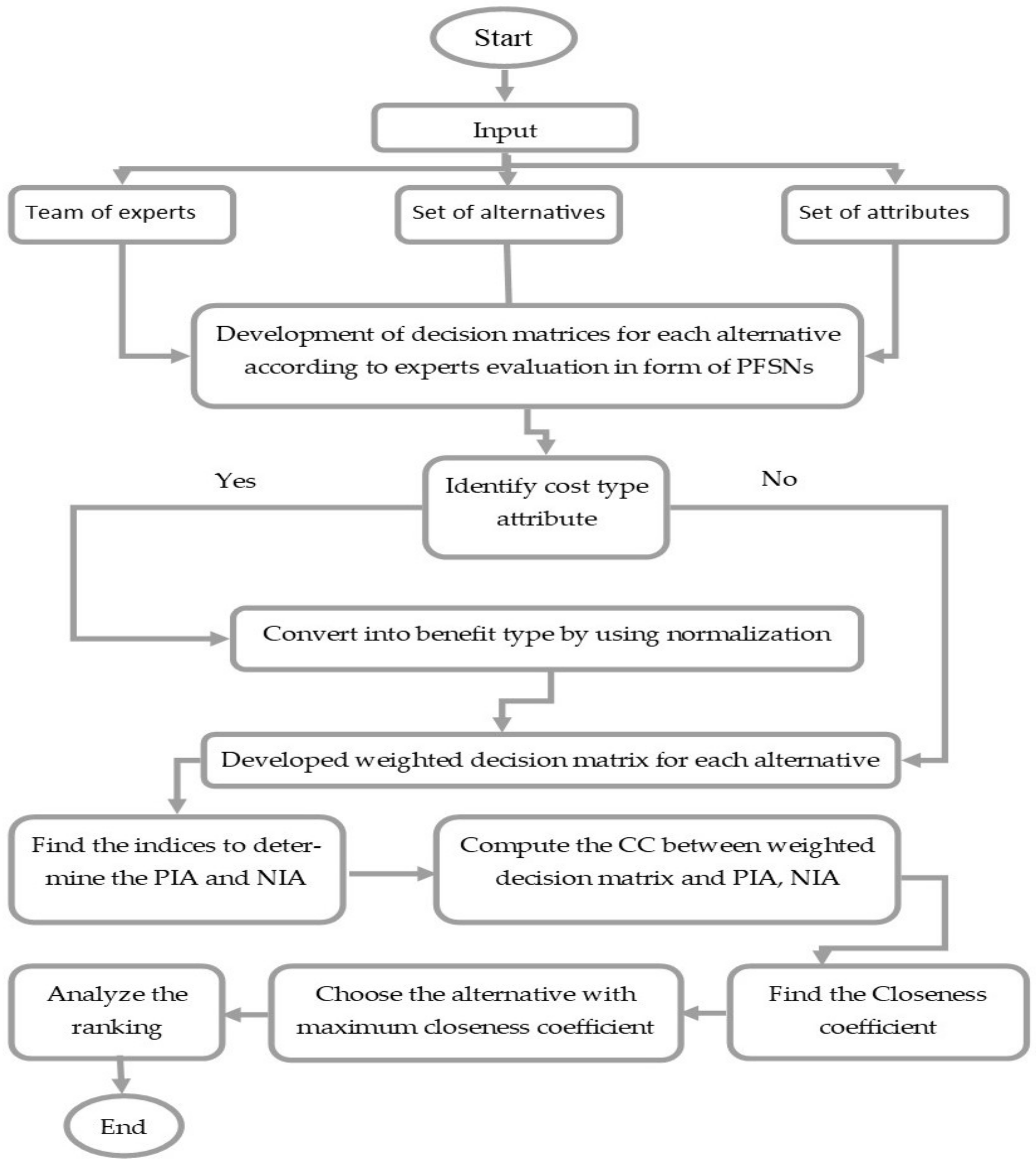
4.1. Proposed Methodology for Selection of Green Supplier Chain Management

Let a collection of “$s$” alternatives such as $\beta$ = $\left\{{\beta }^1, {\beta }^2, {\beta }^3,\dots , {\beta }^s\right\}$ be assessed by a team of experts, such as $\mathcal{U}$ = $\left\{u_1, u_2, u_3,\dots , u_n\right\}$ with weights $\Omega$ = ${({\Omega }_1, {\Omega }_1,\dots , {\Omega }_n)}^T$, such that ${\Omega }_i$ $>$ 0, ${{\displaystyle \sum }}_{i=1}^n{\Omega }_i$ = 1. Let $ℰ$ = $\left\{e_1, e_2,\dots , e_m\right\}$ be a set of attributes with weights γ = ${({\mathsf{\gamma }}_1,{ \mathsf{\gamma }}_2,{ \mathsf{\gamma }}_3,\dots ,{ \mathsf{\gamma }}_m)}^T$ express the weights of parameters like ${\mathsf{\gamma }}_j$ $>$ 0, ${{\displaystyle \sum }}_{j=1}^m{\mathsf{\gamma }}_j$ = 1. The team of experts {$u_i$: $i$ = 1, 2,…, $n$} evaluates the alternatives {${\beta }^{(z)}$: $z$ = 1, 2, …, $s$} under the considered parameters {${\mathrm{e}}_j$: $j$ = 1, 2, …, $m$}, given in the form of PFSNs, such as ${ℒ}_{ij}^{(z)}$ = $({\mathcal{T}}_{ij}^{(z)}, {\mathcal{J}}_{ij}^{(z)})$, where 0 $\le$ ${\mathcal{T}}_{ij}^{(z)}, {\mathcal{J}}_{ij}^{(z)}$ $\le$ 1 and ${({\mathcal{T}}_{ij}^{(z)})}^2$+ ${({\mathcal{J}}_{ij}^{(z)})}^2$ $\le$ 1. So ${ℒ}_{ij}^{(z)}$ = $({\mathcal{T}}_{ij}^{(z)}, {\mathcal{J}}_{ij}^{(z)})$ for all $i$, $j$ is also a PFSN.

Step 1. Acquire a decision matrix $D^{(z)}$ = ${ℒ}_{ij}^{(z)}$ = $({\mathcal{T}}_{ij}^{(z)}, {\mathcal{J}}_{ij}^{(z)})$ from experts for each alternative {${\beta }^{(z)}$: $z$ = 1, 2, …, $s$} such as:

$$\begin{gathered} \begin{array}{cccc}{e}_1& e_2& \dots ..& e_m\end{array} \\ {D}^{(z)} = {({\beta }^{(z)}, ℰ)}_{n\times m}= \begin{array}{c}{u}_1\\ u_2\\ ⋮\\ u_n\end{array} \left(\begin{array}{cccc}\left({\mathcal{T}}_{11}^{\left(z\right)}, {\mathcal{J}}_{11}^{\left(z\right)}\right)& \left({\mathcal{T}}_{12}^{\left(z\right)}, {\mathcal{J}}_{12}^{\left(z\right)}\right)& \cdots & \left({\mathcal{T}}_{1m}^{\left(z\right)}, {\mathcal{J}}_{1m}^{\left(z\right)}\right)\\ \left({\mathcal{T}}_{21}^{\left(z\right)}, {\mathcal{J}}_{21}^{\left(z\right)}\right)& \left({\mathcal{T}}_{22}^{\left(z\right)}, {\mathcal{J}}_{22}^{\left(z\right)}\right)& \cdots & \left({\mathcal{T}}_{2m}^{\left(z\right)}, {\mathcal{J}}_{2m}^{\left(z\right)}\right)\\ ⋮& ⋮& ⋮& ⋮\\ \left({\mathcal{T}}_{n1}^{\left(z\right)}, {\mathcal{J}}_{n1}^{\left(z\right)}\right)& \left({\mathcal{T}}_{n2}^{\left(z\right)}, {\mathcal{J}}_{n2}^{\left(z\right)}\right)& \cdots & \left({\mathcal{T}}_{nm}^{\left(z\right)}, {\mathcal{J}}_{nm}^{\left(z\right)}\right)\end{array}\right) \end{gathered}$$

(9)

Step 2. Obtain the usual Pythagorean fuzzy soft decision matrix. In it, the resulting matrix ${(D^{(z)})}_{n\times m}$ is assessed with two types of attributes, i.e., a benefit attribute (${\Delta }_b$) and cost attributes ${\Delta }_c$. If all the attributes are of the same type, there is no need to normalize the rating values, whereas if there are different benefit type and cost type attributes in the MCDM, then the following normalization formula may be used to standardize the performance rating matrix ${(D^{(z)})}_{n\times m}$ into a normalized matrix ${(R_{ij}^{(z)})}_{n\times m}$.

$$R_{ij}^{(z)} = \{\begin{array}{c}{ℒ}_{e_{ij}}^c=({\mathcal{J}}_{ij}, {\mathcal{T}}_{ij}); cost type parameter\\ {ℒ}_{e_{ij}}=({\mathcal{T}}_{ij}, {\mathcal{J}}_{ij}); benefit type parameter\end{array}$$

where ${ℒ}_{e_{ij}}^c$ is the complement of ${ℒ}_{e_{ij}}$.

Step 3. Develop the weighted decision matrix ${\overline{\beta }}^{(z)}$ = ${({\overline{R}}_{ij}^{(z)})}_{n\times m}$, where

$${\overline{R}}_{ij}^{(z)} = {\mathsf{\gamma }}_j{\Omega }_i{R}_{ij}^{(z)} = (\sqrt{1-{({(1-{\mathcal{T}}^2)}^{{\Omega }_i})}^{{\mathsf{\gamma }}_j}}, {({(\mathcal{J})}^{{\Omega }_i})}^{{\mathsf{\gamma }}_j}) = ({\overline{\mathcal{T}}}_{ij}^{(z)}, {\overline{\mathcal{J}}}_{ij}^{(z)})$$

(10)

Here, ${\Omega }_i$ is the weight of the $i\mathrm{th}$ expert and ${\mathsf{\gamma }}_j$ is the weight for the $j\mathrm{th}$ parameter.

Step 4. Compute the indices like ${\mathcal{h}}_{ij}$ = arg $ma{x}_z\left\{{\theta }_{ij}^{(z)}\right\}$ and $g_{ij}$ = arg $mi{n}_z\left\{{\theta }_{ij}^{(z)}\right\}$ and find the PIA and NIA based on indices, as follows:

$${ℒ}^{+} = {({\mathcal{T}}^{+}, {\mathcal{J}}^{+})}_{n\times m} = ({\overline{\mathcal{T}}}_{ij}^{(h_{ij})}, {\overline{\mathcal{J}}}_{ij}^{(h_{ij})})$$

(11)

and

$${ℒ}^{-} = {({\mathcal{T}}^{-}, {\mathcal{J}}^{-})}_{n\times m} = ({\overline{\mathcal{T}}}_{ij}^{(g_{ij})}, {\overline{\mathcal{J}}}_{ij}^{(g_{ij})})$$

(12)

Step 5. Find the CC among individual alternatives of weighted decision matrices ${\overline{\beta }}^{(z)}$ and PIA ${ℒ}^{+}$.

$$\begin{array}{c}{p}^{(z)} = {\delta }_{PFSS}({\overline{\beta }}^{(z)}, {ℒ}^{+}) = \frac{{\mathcal{C}}_{PFSS}({\overline{\beta }}^{(z)}, {ℒ}^{+}) }{\sqrt{{Ϛ}_{PFSS}{\overline{\beta }}^{(z)}\ast {Ϛ}_{PFSS}{ℒ}^{+}}} = \\ \frac{{{\displaystyle \sum }}_{j=1}^m{{\displaystyle \sum }}_{i=1}^n({\overline{\mathcal{T}}}_{ij}^{(z)} \ast {\mathcal{T}}^{+}+ {\overline{\mathcal{J}}}_{ij}^{(z)}\ast {\mathcal{J}}^{+})}{\sqrt{{{\displaystyle \sum }}_{j=1}^m{{\displaystyle \sum }}_{i=1}^n({({\overline{\mathcal{T}}}_{ij}^{(z)})}^2+ {({\overline{\mathcal{J}}}_{ij}^{(z)})}^2)}\sqrt{{{\displaystyle \sum }}_{j=1}^m{{\displaystyle \sum }}_{i=1}^n({({\mathcal{T}}^{+})}^2+ {({\mathcal{J}}^{+})}^2)}}\end{array}$$

(13)

Step 6. Find the CC among individual alternative weighted decision matrices, ${\overline{\beta }}^{(z)}$ and NIA ${ℒ}^{-}$.

$$\begin{array}{c}{q}^{(z)} = {\delta }_{PFSS}({\overline{\beta }}^{(z)}, {ℒ}^{-})=\frac{{\mathcal{C}}_{PFSS}({\overline{\beta }}^{(z)}, {ℒ}^{-}) }{\sqrt{{Ϛ}_{PFSS}{\overline{\beta }}^{(z)}\ast {Ϛ}_{PFSS}{ℒ}^{-}}} = \\ \frac{{{\displaystyle \sum }}_{j=1}^m{{\displaystyle \sum }}_{i=1}^n({\overline{\mathcal{T}}}_{ij}^{(z)} \ast {\mathcal{T}}^{-}+ {\overline{\mathcal{J}}}_{ij}^{(z)}\ast {\mathcal{J}}^{-})}{\sqrt{{{\displaystyle \sum }}_{j=1}^m{{\displaystyle \sum }}_{i=1}^n({({\overline{\mathcal{T}}}_{ij}^{(z)})}^2+ {({\overline{\mathcal{J}}}_{ij}^{(z)})}^2)}\sqrt{{{\displaystyle \sum }}_{j=1}^m{{\displaystyle \sum }}_{i=1}^n({({\mathcal{T}}^{-})}^2+ {({\mathcal{J}}^{-})}^2)}}\end{array}$$

(14)

Step 7. Compute the closeness coefficient for each alternative:

$${ℛ}^{(z)} = \frac{\mathcal{K}({\overline{\beta }}^{(z)}, {ℒ}^{-})}{\mathcal{K}({\overline{\beta }}^{(z)}, {ℒ}^{+})+\mathcal{K}({\overline{\beta }}^{(z)}, {ℒ}^{-})}$$

(15)

where $\mathcal{K}({\overline{\beta }}^{(z)}, {ℒ}^{-})$ = 1 $-$ $q^{(z)}$ and $\mathcal{K}({\overline{\beta }}^{(z)}, {ℒ}^{+})$ = 1 $-$ $p^{(z)}$.

Step 8. Pick the alternative according to the supreme value of the closeness coefficient.

Step 9. Rank the alternatives and choose the best one.

A flowchart of the proposed TOPSIS algorithm is presented in Figure 1.

4.2. Application of the Proposed Technique for Green Supplier Chain Management

Case Study

Destruction of the natural environment, as well as air and water pollution have serious effects on plants, wildlife, and human life, showing correlations with ischemic diseases vascular disease, lung cancer, chronic obstructive lung disease, stroke, guinea worm disease, cholera, tuberculosis, and typhoid fever. The green supply chain seeks to minimize environmental degradation and regulate air, water, and waste contamination. The fundamental idea behind the green concept is to expand environmental protection. Firms which adopt the green concept are seeking to “kill two birds with one bird stone”, i.e., to reduce environmental pollution as well as manufacturing costs. Sustainability or the green supply chain concept is predicated upon the idea that supportable apparatuses need to be unified into a well-ordered process [64,65,66,67], comprising procurement, assembly, ordering, manufacturing, delivery, and waste management. Globally, firms have been facing tremendous pressure from governments as well as consumers; companies which have combined their operational practices with sustainable development in terms of services and manufacturing processes possess a competitive advantage. During the past few decades, the increasing effects of global warming, climate change, waste disposal, and air pollution have motivated professionals to think in a more environmentally friendly manner [68]. Rath [69] represented GSCM as a catalyst for sustainable development. Due to environmental problems, GSCM is dependent upon a permanent, broad interest in developing nations if it is to continue to grow. Developing nations have recently become part of the green environment campaign. Managers of the green supply chain must be in a position to influence the design, procurement, distribution, and disposal of the relevant products.

The reverse logistics activity model enhances environmental, social and economic performance of the green supply chain. However, when reverse logistics are included, the GSCM strategy is not profitable. Reverse logistics describes the procedure of possession allocation, e.g., reuse, recapture, or refinement. Products move from suppliers to end-users in supply chain networks. The efficiency of that flow is calculated by supply chain staff using time delivery indicators. This is an important index for the supply chain aimed at ensuring fast and efficient distribution to the end customer from the moment he/she places an order. Reverse logistics is a more advanced approach compared to progressive logistics. Historically, reverse logistics has often been misunderstood or overlooked; however, this is no longer the case. Companies which have no projected reverse logistics plans may also have gloomy economic outlooks. Eco-management should be applied to the entire customer order cycle, including design, procurement, assembly, publicity, and transport [70]. GSCM, the definition of which has evolved over the years [71], integrates environmental protection within supply chain management to enhance environmental sustainability through numerous green procedures [72]. The following concepts may be said to characterize GSCM: Sustainable management of the supply network [73]; Sustainability of supply and demand across corporate social responsibility networks [74]; Environmental Supply Chain Management [75]; Green procurement [76]; and Green logistics [77].

In recent years, the multidisciplinary field of GSCM has been the focus of academia and industry. Development occurs through the study of problems. Ongoing academic development in this field comes in the form of new ideas and a mindsets. Suppliers provide goods, services, or products, but companies cannot provide raw materials. Manufacturers are an indispensable part of supply chains, ideally providing consumers with products of appropriate quality, quantity, and price within a predetermined time. In the past few years, environmental factors have changed and vital issues for decision-makers have appeared. Waste electrical and electronic equipment (WEEE), restrictions on the use of hazardous substances (RoHS), and eco-design standards for energy use projects have become the three major European union regulations related to e-commerce. This indicates that the EU is concerned about recycling, pollutants, low energy consumption, and wasting resources. Recently, Riaz et al. [78] presented the q-rung orthopair fuzzy notion with some prioritized AOs, and presented a DM approach to solving MCGDM concerns under a specific environment. They then utilized this approach for supplier selection in GSCM by considering alternative approaches for the disposal of electrical and electronic equipment. Rao [79] identified GSCM as a screening process in which suppliers were assessed in terms of their environmental performance and compliance with environmental regulations. Supplier selection based on GSCM will enhance environmental protection. Since the company focuses primarily on suppliers, it must adopt multiple methods to evaluate its green measures. Supplier selection should consider various objectives; in this sense, in 2002, Bhutta and Huq [80] recommended selecting a supplier which could be regarded as a CDM.

Srivastava [81] presented a comprehensive definition of GSCM, i.e., acknowledgment of environmental considerations regarding supply chain management, including product design, the selection and procurement of materials, manufacturing process, product packaging, and scrap management. For an enterprise, GSCM has many advantages. The argument that becoming more ecologically minded leads to lower sales and higher operating costs has been refuted, and many companies have now realized that they will not be able to satisfy their clients’ wishes if they fail to incorporate environmental initiatives in their supply chain. Connections between ecology and financial incentives have been developed by many companies. Companies have gained insights into their supply chains and found areas that can be changed to increase income. Green logistics helps to reduced emissions such as CO2 and CO. The use of fossil fuels has been devastating for the environment; air travel, for example, is highly polluting. In a literature review, we examined the factors influencing green supplier selection according to different researchers. The selection standards for green suppliers are given in

Table 1. Standards for assessing the disposal of electrical and electronic equipment; constraint of hazardous ingredients.

Criteria	Definition
Quality	Reject rate, upgrading procedure, guarantee coverage and rights, and superiority assurance.
Distribution	Percentage to achieve order, principal period, as well as order regularity
Services	Accountability, organization record, and readiness.
Atmosphere	Eco-design stipulations, compounds containing ozone-depleting chemicals
Corporate societal concern	Worker freedom and constitutional rights, investor constitutional rights, information regulations, and respect for superiors.

.

4.3. Numerical Example

Let {${\beta }^{(1)}$, ${\beta }^{(2)}$, ${\beta }^{(3)}$, ${\beta }^{(4)}$, ${\beta }^{(5)}$} be a set of alternatives and ${\mathfrak{e}}_1$ = Quality, ${\mathfrak{e}}_2$ = Distribution, ${\mathfrak{e}}_3$ = Services, ${\mathfrak{e}}_4$ = Atmosphere, and ${\mathfrak{e}}_5$ = Corporate societal concern, with weights ${(0.25, 0.15, 0.20, 0.10,0.30)}^T$. Then, {$u_1$, $u_2$, $u_3$} is a set of experts who will evaluate the best alternative with weight vector ${(0.243, 0.514, 0.343)}^T$. The team of experts evaluates the alternatives according to the aforementioned parameters. Each expert evaluates the ratings for alternatives in PFSNs according to the considered parameters see

Table 2. PFS Decision Matrix for ${\beta }^{(1)}$.

${\mathit{\beta }}^{(1)}$	${\mathfrak{e}}_1$	${\mathfrak{e}}_2$	${\mathfrak{e}}_3$	${\mathfrak{e}}_4$	${\mathfrak{e}}_5$
${\mathit{u}}_{\mathbf{1}}$	$(0.7, 0.4)$	$(0.7, 0.2)$	$(0.9, 0.2)$	$(0.5, 0.4)$	$(0.4, 0.5)$
${\mathit{u}}_{\mathbf{2}}$	$(0.4, 0.7)$	$(0.3, 0.6)$	$(0.6, 0.7)$	$(0.3, 0.8)$	$(0.8, 0.3)$
${\mathit{u}}_{\mathbf{3}}$	$(0.5, 0.4)$	$(0.4, 0.3)$	$(0.7, 0.5)$	$(0.7, 0.5)$	$(0.6, 0.4)$
${\mathit{\beta }}^{(\mathbf{2})}$
${\mathit{u}}_{\mathbf{1}}$	$(0.7, 0.3)$	$(0.6, 0.5)$	$(0.3, 0.6)$	$(0.7, 0.4)$	$(0.6, 0.4)$
${\mathit{u}}_{\mathbf{2}}$	$(0.8, 0.3)$	$(0.7, 0.4)$	$(0.7, 0.3)$	$(0.4, 0.8)$	$(0.6, 0.4)$
${\mathit{u}}_{\mathbf{3}}$	$(0.6, 0.5)$	$(0.6, 0.2)$	$(0.6, 0.1)$	$(0.7, 0.4)$	$(0.4, 0.5)$
${\mathit{\beta }}^{(\mathbf{3})}$
${\mathit{u}}_{\mathbf{1}}$	$(0.3, 0.8)$	$(0.4, 0.6)$	$(0.3, 0.6)$	$(0.5, 0.6)$	$(0.4, 0.5)$
${\mathit{u}}_{\mathbf{2}}$	$(0.3, 0.6)$	$(0.5, 0.7)$	$(0.6, 0.5)$	$(0.5, 0.4)$	$(0.4, 0.5)$
${\mathit{u}}_{\mathbf{3}}$	$(0.7, 0.4)$	$(0.7, 0.2)$	$(0.9, 0.2)$	$(0.5, 0.4)$	$(0.4, 0.5)$
${\mathit{\beta }}^{(\mathbf{4})}$
${\mathit{u}}_{\mathbf{1}}$	$(0.8, 0.3)$	$(0.5, 0.5)$	$(0.5, 0.4)$	$(0.5, 0.6)$	$(0.4, 0.7)$
${\mathit{u}}_{\mathbf{2}}$	$(0.3, 0.5)$	$(0.5, 0.3)$	$(0.7, 0.2)$	$(0.8, 0.4)$	$(0.3, 0.7)$
${\mathit{u}}_{\mathbf{3}}$	$(0.6, 0.2)$	$(0.2, 0.5)$	$(0.3, 0.5)$	$(0.6, 0.4)$	$(0.5, 0.5)$
${\mathit{\beta }}^{(\mathbf{5})}$
${\mathit{u}}_{\mathbf{1}}$	$(0.6, 0.3)$	$(0.3, 0.8)$	$(0.5, 0.6)$	$(0.4, 0.2)$	$(0.5, 0.5)$
${\mathit{u}}_{\mathbf{2}}$	$(0.8, 0.5)$	$(0.6, 0.5)$	$(0.6, 0.3)$	$(0.4, 0.8)$	$(0.7, 0.5)$
${\mathit{u}}_{\mathbf{3}}$	$(0.3, 0.4)$	$(0.4, 0.6)$	$(0.7, 0.3)$	$(0.6, 0.5)$	$(0.7, 0.4)$

and

Table 3. Weighted PFS decision matrix for alternatives.

${\overline{\mathit{\beta }}}^{(1)}$	${\mathfrak{e}}_1$	${\mathfrak{e}}_2$	${\mathfrak{e}}_{\mathbf{3}}$	${\mathfrak{e}}_{\mathbf{4}}$	${\mathfrak{e}}_5$
${\mathit{u}}_{\mathbf{1}}$	$(0.78949, 0.89464)$	$(0.86778, 0.88929)$	$(0.94637, 0.85519)$	$(0.87392, 0.95645)$	$(0.62041, 0.90388)$
${\mathit{u}}_{\mathbf{2}}$	$(0.73559, 0.91241)$	$(0.79548, 0.92425)$	$(0.85344, 0.92929)$	$(0.85852, 0.97732)$	$(0.87434, 0.68983)$
${\mathit{u}}_{\mathbf{3}}$	$(0.74408, 0.85458)$	$(0.80777, 0.88348)$	$(0.85395, 0.90928)$	$(0.85395, 0.95356)$	$(0.74613, 0.82814)$
${\overline{\mathit{\beta }}}^{(\mathbf{2})}$
${\mathit{u}}_{\mathbf{1}}$	$(0.78949, 0.86391)$	$(0.84312, 0.95072)$	$(0.68473, 0.95156)$	$(0.90979, 0.95645)$	$(0.71086, 0.87494)$
${\mathit{u}}_{\mathbf{2}}$	$(0.89413, 0.73387)$	$(0.91194, 0.86824)$	$(0.88434, 0.78072)$	$(0.88441, 0.97732)$	$(0.78842, 0.75383)$
${\mathit{u}}_{\mathbf{3}}$	$(0.78345, 0.88792)$	$(0.86379, 0.84738)$	$(0.82264, 0.72912)$	$(0.85395, 0.93908)$	$(0.65248, 0.86706)$
${\overline{\mathit{\beta }}}^{(\mathbf{3})}$
${\mathit{u}}_{\mathbf{1}}$	$(0.62287, 0.97325)$	$(0.78766, 0.96345)$	$(0.68473, 0.95156)$	$(0.87392, 0.97548)$	$(0.62041, 0.90388)$
${\mathit{u}}_{\mathbf{2}}$	$(0.68294, 0.87697)$	$(0.86171, 0.94649)$	$(0.85344, 0.86718)$	$(0.90554, 0.91011)$	$(0.69177, 0.80754)$
${\mathit{u}}_{\mathbf{3}}$	$(0.82091, 0.85458)$	$(0.88833, 0.84738)$	$(0.91997, 0.80187)$	$(0.88848, 0.93908)$	$(0.65248, 0.86706)$
${\overline{\mathit{\beta }}}^{(\mathbf{4})}$
${\mathit{u}}_{\mathbf{1}}$	$(0.82749, 0.86391)$	$(0.81697, 0.95072)$	$(0.87392, 0.91479)$	$(0.87392, 0.97548)$	$(0.62041, 0.94933)$
${\mathit{u}}_{\mathbf{2}}$	$(0.68294, 0.83683)$	$(0.86171, 0.83056)$	$(0.88434, 0.71828)$	$(0.95623, 0.91011)$	$(0.63278, 0.89584)$
${\mathit{u}}_{\mathbf{3}}$	$(0.78345, 0.75879)$	$(0.72567, 0.93116)$	$(0.70841, 0.90928)$	$(0.90699, 0.93908)$	$(0.70136, 0.86706)$
${\overline{\mathit{\beta }}}^{(\mathbf{5})}$
${\mathit{u}}_{\mathbf{1}}$	$(0.75246, 0.86391)$	$(0.75273, 0.98386)$	$(0.87392, 0.95156)$	$(0.85289, 0.92476)$	$(0.66744, 0.90388)$
${\mathit{u}}_{\mathbf{2}}$	$(0.89413, 0.83683)$	$(0.88793, 0.89863)$	$(0.85344, 0.78072)$	$(0.88441, 0.97732)$	$(0.83163, 0.80754)$
${\mathit{u}}_{\mathbf{3}}$	$(0.64991, 0.85458)$	$(0.80777, 0.94879)$	$(0.85395, 0.84774)$	$(0.90699, 0.95356)$	$(0.78914, 0.82814)$

. The proposed technique to find the best alternative is described in Section 4.1.

Step 1. Develop decision matrices for each alternative regarding expert opinion in PFSN by applying a set of parameters.

Step 2. No need for normalization because all parameters are of the same type.

Step 3. By utilizing Equation (10), it is possible to develop a weighted decision matrix for each alternative ${\overline{\beta }}^{(z)}$ = ${({\overline{R}}_{ij}^{(z)})}_{n\times m}$.

Step 4. Compute the PIA and NIA using Equations (11) and (12), respectively.

$$\begin{gathered} {ℒ}^{+}= \left[\begin{array}{ccccc}(0.62287, 0.97325)& (0.75273, 0.98386)& (0.68473, 0.95156)& (0.87392, 0.97548)& (0.62041, 0.94933)\\ (0.68294, 0.87697)& (0.79548, 0.92425)& (0.85344, 0.92929)& (0.85852, 0.97732)& (0.63278, 0.89584)\\ (0.64991, 0.85458)& (0.72567, 0.93116)& (0.70841, 0.90928)& (0.85395, 0.95356)& (0.65248, 0.86706)\end{array}\right] \\ {ℒ}^{-} = \left[\begin{array}{ccccc}(0.82749, 0.86391)& (0.86778, 0.88929)& (0.94637, .85519)& (0.90979, 0.95645)& (0.71086, 0.87494)\\ (0.89413, 0.73387)& (0.91194, 0.86824)& (0.88434, .71828)& (0.95623, 0.91011)& (0.87434, 0.68983)\\ (0.78345, 0.75879)& (0.88833, 0.84738)& (0.91997, .80187)& (0.90699, 0.93908)& (0.78914, 0.82814)\end{array}\right] \end{gathered}$$

Step 5. Calculate the CC among ${\overline{\beta }}^{(z)}$ and PIA ${ℒ}^{+}$ using Equation (13), given as $p^{(1)}$ = 0.99349, $p^{(2)}$ = 0.99228, $p^{(3)}$ = 0.99652, $p^{(4)}$ = 0.99524, $p^{(5)}$ = 0.99255.

Step 6. Calculate the CC among ${\overline{\beta }}^{(z)}$ and NIA ${ℒ}^{-}$ using Equation (14), given as $q^{(1)}$ = 0.99579, $q^{(2)}$ = 0.99632, $q^{(3)}$ = 0.99244, $q^{(4)}$ = 0.99346, $q^{(5)}$ = 0.99678.

Step 7. Compute the closeness coefficient using Equation (15).

${ℛ}^{(1)}$ = 0.39272, ${ℛ}^{(2)}$ = 0.32281, ${ℛ}^{(3)}$ = 0.68478, ${ℛ}^{(4)}$ = 0.57876, and ${ℛ}^{(5)}$ = 0.30178.

Step 8. Choose the alternative with maximum closeness coefficient ${ℛ}^{(3)}$ = 0.68478, so ${\beta }^{(3)}$ is the best alternative.

Step 9. Ranking the alternatives, we can see ${ℛ}^{(3)}$ $>$ ${ℛ}^{(4)} >{ℛ}^{(1)}$ $>$ ${ℛ}^{(2)}>$ ${ℛ}^{(5)}$, so the ranking of the alternatives is ${\beta }^{(3)}$ $>$ ${\beta }^{(4)} >{\mathfrak{ß}}^{(1)}$ $>$ ${\beta }^{(2)}>$ ${\beta }^{(5)}$.

5. Discussions and Comparative Analysis

In this section, we are going to talk about the effectiveness, simplicity, tractability, and benefits of the proposed approach. We also presented a brief comparison between the proposed approach with some existing techniques.

5.1. Superiority of the Proposed Method

Zadeh’s FS deals with uncertainty by utilizing MD of alternatives, as discussed in [1], but it cannot provide information about the NMD of the alternatives under considered parameters. Zhang et al. [65] and Xu et al. [66] deal with uncertainty by using MD and NMD. But these theories cannot deal with situations where the sum of MD and NMD exceeds one. On the other hand, our technique can accommodate more vagueness comparative to those theories by upgrading the $MD +$ $NMD\le 1$ to $M{D}^2 +$ $NM{D}^2\le 1$. Yager [29,30] PFS accommodates more uncertainty comparative to IFS, but it cannot deal with parametrization. Maji et al. [6] extended FSS to resolve uncertain problems via MD along with parametric values, but FSS cannot deal with the NMD of the parameters of the alternative. To overcome these hurdles, Maji et al. [7] proposed an IFSS which accommodates uncertainty by using the MD and NMD of the parameters of the alternative, such as $MD +$ $NMD\le 1$. IFSS competently handles uncertain and vague information compared to FS, FSS, and IFS. Sometimes IFSS is unable to deal with situations in which the sum of MD and NMD exceeds 1. But, our proposed technique can easily solve these obstacles and present more operational advantages in the DM process. Many hybrid structures of FS and IFS become special cases of PFSSs after certain conditions are added. Among them, when data associated with the object is expressed exactly and empirically (see

Table 4. Comparison of PFSSs with some existing theories.

	Set	Truth Information	Falsity	Loss of Information	Parametrization	Advantages	Limitations
Zadeh [1]	FS	✓	×	✓	×	Deals with uncertainty by using fuzzy interval	Cannot deal with NMD
Zhang et al. [65]	IFS	✓	✓	✓	×	Deals with uncertainty by using MD and NMD	Cannot deal with problems that satisfies 1 $<$ $\mathrm{MD}+$ $\mathrm{NMD} \le$ 0
Xu et al. [66]	IFS	✓	✓	×	×	Deals with uncertainty by using MD and NMD	Cannot deal with problems that satisfies 1 $<$ $\mathrm{MD}+$ $\mathrm{NMD} \le$ 0
Yager [29,30]	PFS	✓	✓	×	×	Deals better with uncertainty compared to IFS	Cannot deal with problems that satisfy 1 $<$ ${\mathrm{MD}}^2+$ $\mathrm{N}{\mathrm{MD}}^2$ $\le$ 0
Maji et al. [6]	FSS	✓	×	✓	✓	Deals with uncertainty by using MD with parametrization	Cannot deal with NMD of the parameters
Maji et al. [7]	IFSS	✓	✓	×	✓	Deals with uncertainty by using MD and NMD with parametrization	Cannot deal with problems that satisfy 1 $<$ $\mathrm{MD}+$ $\mathrm{NMD} \le$ 0
Proposed approach	PFSSs	✓	✓	×	✓	Deals better with uncertainty compared to IFSS	Cannot deal with problems that satisfy 1 $<$ ${\mathrm{MD}}^2+{\mathrm{NMD}}^2\le$ 0

), they can be quite appropriate tools with which to syndicate imprecise as well as uncertain information in DM procedures. Through this research and comparison, we determined that outcomes obtained by the proposed approach are more accurate than those obtained using other techniques. However, the presented DM technique accommodates a lot of information to address the anxiety in the data comparative to other methodologies. Hence, our proposed method is effective, flexible, simple, and superior to other hybrid structures of fuzzy sets and intuitionistic fuzzy sets.

5.2. Comparative Analysis

Through the exploration of the studies mentioned above, it was concluded that the outcomes through the proposed approach overlap with those of techniques; therefore, the established TOPSIS technique competently deals with uncertain and vague information compared to existing techniques. However, with regard to existing decision-making techniques, the main benefit of the planned approach is that it accommodates more information in order to deal with uncertainty in the data. For example, information associated with objects could be stated more precisely and objectively. It is also a useful tool for solving imprecise and incomprehensible information in the DM process. Additionally, a comparative analysis showed that the calculation process of the proposed approach is not the same as those in other techniques. This is due to the determination of PIA and NIA. In existing techniques, PIA and NIA are conceptualized according to a given distance and similarity measures. Therefore, the inspiration for the score value corresponding to each parameter will not affect other parameters, so information loss will occur in the process. On the other hand, in our method, PIA and NIA are calculated based on the inspiration of the maximum CC on a given substitution level, and as such, there is no serious loss of information. The intensity of each ideal correlation measure is obtained from the assessment explanations, so to find the superlative result, it is simply a matter of computing the correlation between them. The benefit of the planned TOPSIS method over existing methods is that it notices not just the degree of discrimination, but also the degree of similarity between observations, thereby avoiding decisions based on negative factors. Finally, the ranks of all alternatives using the existing operators yielded the same final decision, that is, ${\beta }^{(3)}$ was selected for GSCM. All rankings were also calculated by applying existing methods. The proposed method was also compared with other methods, such as those of Zhang [34], Garg [35], Ma and Xu [38], and Bailey et al. [82] weighted Pearson CC (WPCC). The comparison results are listed below (see

Table 5. Comparative analysis with existing operators.

Method	Score Values for Alternatives					Ranking Order
	${\mathit{\beta }}^{(1)}$	${\mathit{\beta }}^{(2)}$	${\mathit{\beta }}^{(3)}$	${\mathit{\beta }}^{(4)}$	${\mathit{\beta }}^{(5)}$
Zhang [34] PFSWA	0.21173	0.22017	0.33215	0.27008	0.21893	${\beta }^{(3)}$$>$${\beta }^{(4)}>{\beta }^{(2)}$$>$${\beta }^{(5)}>$${\beta }^{(1)}$
Zhang [34] PFSWG	0.20587	0.23066	0.32902	.25462	0.21727	${\beta }^{(3)}$$>$${\beta }^{(4)}>{\beta }^{(2)}$$>$${\beta }^{(5)}>$${\beta }^{(1)}$
Garg [35] PFEWA	0.51686	0.54833	0.60467	0.59021	0.51235	${\beta }^{(3)}$$>$${\beta }^{(4)}>{\beta }^{(2)}$$>$${\beta }^{(1)}>$${\beta }^{(5)}$
Ma and Xu [38] SPFWA	0.08158	0.07674	0.14762	0.09959	0.07985	${\beta }^{(3)}$$>$${\beta }^{(4)}>{\beta }^{(1)}$$>$${\beta }^{(5)}>$${\beta }^{(2)}$
Garg [35] PFEWG	0.54219	0.56597	0.62190	0.59381	0.52209	${\beta }^{(3)}$$>$${\beta }^{(4)}>{\beta }^{(2)}$$>$${\beta }^{(1)}>$${\beta }^{(5)}$
Bailey et al. [82] WPCC	$-0.77177$	$-0.82409$	$-0.76255$	$-0.82597$	$-0.80763$	${\beta }^{(3)}$$>$${\beta }^{(1)}>{\beta }^{(5)}$$>$${\beta }^{(2)}>$${\beta }^{(4)}$
Proposed TOPSIS method	0.39272	0.32281	0.68478	0.57876	0.30178	${\beta }^{(3)}$$>$${\beta }^{(4)}>{\beta }^{(1)}$$>$${\beta }^{(2)}>$${\beta }^{(5)}$

). The best choice made by the proposed method was compared with those of existing methods; this underlined the reliability and effectiveness of our method.

Now, according to the evaluation matrix, various aggregation operators are compared, and the corresponding results of each alternative are given (see Table 5). It can be seen from Table 5 that the alternative ${\beta }^{(3)}$ has excellent substitution for GSCM.

Table 6. Characteristic analysis of some existing operators.

Operator	Fuzzy Information	Parameter Information
PFSWA [34]	✓	×
PFSWG [34]	✓	×
PFEWA [35]	✓	×
SPFWA [38]	✓	×
PFEWG [35]	✓	×
Proposed Approach	✓	✓

indicates the overall characteristics of the proposed method. It can clearly be seen that the strategies specified in [34,35,38] do not provide any information about parameter research. The advantage of the presented approach is that it can explain real-life complications using their parametric features. Therefore, the developed concept can be used to solve DM complexity, in contrast to other operators available in the PFS environment.

6. Conclusions

This study focused on PFSS to solve problems which contain insufficient data, ambiguity, and inconsistencies by considering the degree of membership and nonmembership of the set of parameters. In this research, the concepts of CC and WCC for PFSS were put forward and their properties were investigated in detail. Based on the proposed correlation measure, by considering the attribute set and decision-makers, the TOPSIS method was extended in the Pythagorean fuzzy soft environment. To find the ranking of alternatives, we defined the closeness coefficient under the established TOPSIS method. We defined PFSWA and PFSWG operators and presented a DM method based on the developed TOPSIS technique. To solve the MCGDM problem, a numerical illustration was described using the proposed TOPSIS method for GSCM. Furthermore, a comparative analysis was conducted to justify and present the effectiveness of the proposed method. Consequently, relying upon the obtained results, it can be confidently concluded that the proposed methodology possesses higher stability and usability for decision-makers in the DM process. Future research will concentrate upon presenting numerous other operators under the PFSS environment to solve decision-making issues. Moreover, many other structures, such as topological, algebraic, ordered structures, etc., can also be established and propounded within a given environment. This research has pragmatic boundaries, but may be immensely helpful in real-life contexts, including the medical profession, pattern recognition, economics, etc. We are confident that this article will open new vistas for researchers in this field.

References

1. Zadeh, L.A. Fuzzy Sets. Inf. Control. 1965, 8, 338–353. [Google Scholar] [CrossRef] [Green Version]
2. Atanassov, K. Intuitionistic Fuzzy Sets. Fuzzy Sets Syst. 1986, 20, 87–96. [Google Scholar] [CrossRef]
3. Molodtsov, D. Soft Set Theory First Results. Comput. Math. Appl. 1999, 37, 19–31. [Google Scholar] [CrossRef] [Green Version]
4. Maji, P.K.; Biswas, R.; Roy, A.R. Soft set theory. Comput. Math. Appl. 2003, 45, 555–562. [Google Scholar] [CrossRef] [Green Version]
5. Maji, P.K.; Roy, A.R.; Biswas, R. An Application of Soft Sets in a Decision Making Problem. Comput. Math. Appl. 2002, 44, 1077–1083. [Google Scholar] [CrossRef] [Green Version]
6. Maji, P.K.; Biswas, R.; Roy, A.R. Fuzzy soft sets. J. Fuzzy Math. 2001, 9, 589–602. [Google Scholar]
7. Maji, P.K.; Biswas, R.; Roy, A.R. Intuitionistic fuzzy soft sets. J. Fuzzy Math. 2001, 9, 677–692. [Google Scholar]
8. Garg, H.; Arora, R. Generalized and group-based generalized intuitionistic fuzzy soft sets with applications in decision-making. Appl. Intell. 2018, 48, 343–356. [Google Scholar] [CrossRef]
9. Mahmood, T.; Ali, Z. Entropy measure and TOPSIS method based on correlation coefficient using complex q-rung orthopair fuzzy information and its application to multi-attribute decision making. Soft Comput. 2020, 11, 1–27. [Google Scholar]
10. Chamodrakas, I.; Alexopoulou, N.; Martakos, D. Customer evaluation for order acceptance using a novel class of fuzzy methods based on TOPSIS. Expert Syst. Appl. 2009, 36, 7409–7415. [Google Scholar] [CrossRef]
11. Watrobski, J.; Sałabun, W.; Karczmarczyk, A.; Wolski, W. Sustainable decision-making using the COMET method: An empirical study of the ammonium nitrate transport management. In Proceedings of the 2017 Federated Conference on Computer Science and Information Systems (FedCSIS), Prague, Czech Republic, 3–6 September 2017; IEEE: Piscataway, NJ, USA, 2017; pp. 949–958. [Google Scholar]
12. Sałabun, W.; Karczmarczyk, A. Using the comet method in the sustainable city transport problem: An empirical study of the electric powered cars. Procedia Comput. Sci. 2018, 126, 2248–2260. [Google Scholar] [CrossRef]
13. Kahraman, C.; Çevik, S.; Ates, N.Y.; Gülbay, M. Fuzzy multi-criteria evaluation of industrial robotic systems. Comput. Ind. Eng. 2007, 52, 414–433. [Google Scholar] [CrossRef]
14. Sałabun, W. Assessing the 10-Year Risk of Hard Arteriosclerotic Cardiovascular Disease Events Using the Characteristic Objects Method. Stud. Proc. Pol. Assoc. Knowl. Manag. 2015, 77, 65–76. [Google Scholar]
15. Velasquez, M.; Hester, P.T. An analysis of multi-criteria decision making methods. Int. J. Oper. Res. 2013, 10, 56–66. [Google Scholar]
16. Zavadskas, E.K.; Turskis, Z. Multiple criteria decision making (MCDM) methods in economics: An overview. Technol. Econ. Dev. Econ. 2011, 17, 397–427. [Google Scholar] [CrossRef] [Green Version]
17. Bashir, Z.; Rashid, T.; Watróbski, J.; Sałabun, W.; Malik, A. Hesitant probabilistic multiplicative preference relations in group decision making. Appl. Sci. 2018, 8, 398. [Google Scholar] [CrossRef] [Green Version]
18. Sałabun, W.; Piegat, A. Comparative analysis of MCDM methods for the assessment of mortality in patients with acute coronary syndrome. Artif. Intell. Rev. 2017, 48, 557–571. [Google Scholar] [CrossRef]
19. Karczmarczyk, A.; Jankowski, J.; Watrobski, J. Multi-criteria decision support for planning and evaluation of performance of viral marketing campaigns in social networks. PLoS ONE 2018, 13, e0209372. [Google Scholar] [CrossRef]
20. Sałabun, W.; Watrobski, J.; Shekhovtsov, A. Are MCDA Methods Benchmarkable? A Comparative Study of TOPSIS, VIKOR, COPRAS, and PROMETHEE II Methods. Symmetry 2020, 12, 1549. [Google Scholar] [CrossRef]
21. Garg, H.; Arora, R. Maclaurin symmetric mean aggregation operators based on t-norm operations for the dual hesitant fuzzy soft set. J. Ambient Intell. Humaniz. Comput. 2020, 11, 375–410. [Google Scholar] [CrossRef]
22. Arora, R.; Garg, H. A robust correlation coefcient measure of dual hesistant fuzzy soft sets and their application in decision making. Eng. Appl. Artif. Intell. 2018, 72, 80–92. [Google Scholar] [CrossRef]
23. Arora, R.; Garg, H. Group decision-making method based on prioritized linguistic intuitionistic fuzzy aggregation operators and its fundamental properties. Comput. Appl. Math. 2019, 38, 1–36. [Google Scholar] [CrossRef]
24. Garg, H.; Arora, R. Generalized Maclaurin symmetric mean aggregation operators based on Archimedean t-norm of the intuitionistic fuzzy soft set information. Artif. Intell. Rev. 2020, 1–41. [Google Scholar] [CrossRef]
25. Riaz, M.; Sałabun, W.; Farid, H.M.A.; Ali, N.; Watrobski, J. A Robust q-Rung Orthopair Fuzzy Information Aggregation Using Einstein Operations with Application to Sustainable Energy Planning Decision Management. Energies 2020, 13, 2155. [Google Scholar] [CrossRef]
26. Faizi, S.; Sałabun, W.; Ullah, S.; Rashid, T.; Watrobski, J. A New Method to Support Decision-Making in an Uncertain Environment Based on Normalized Interval-Valued Triangular Fuzzy Numbers and COMET Technique. Symmetry 2020, 12, 516. [Google Scholar] [CrossRef] [Green Version]
27. Garg, H.; Arora, R. TOPSIS method based on correlation coefficient for solving decision-making problems with intuitionistic fuzzy soft set information. Aims Math. 2020, 5, 2944–2966. [Google Scholar] [CrossRef]
28. Zulqarnain, R.M.; Xin, X.L.; Saeed, M. Extension of TOPSIS method under intuitionistic fuzzy hypersoft environment based on correlation coefficient and aggregation operators to solve decision making problem. Aims Math. 2020, 6, 2732–2755. [Google Scholar] [CrossRef]
29. Yager, R.R. Pythagorean fuzzy subsets. In Proceedings of the 2013 Joint IFSA World Congress and NAFIPS Annual Meeting, Edmonton, AB, Canada, 24–28 June 2013; pp. 57–61. [Google Scholar]
30. Yager, R.R. Pythagorean membership grades in multicriteria decision making. IEEE Trans. Fuzzy Syst. 2014, 22, 958–965. [Google Scholar] [CrossRef]
31. Zhang, X.; Xu, Z. Extension of topsis to multiple criteria decision making with pythagorean fuzzy sets. Int. J. Intell. Syst. 2014, 29, 1061–1078. [Google Scholar] [CrossRef]
32. Wei, G.; Lu, M. Pythagorean fuzzy power aggregation operators in multiple attribute decision making. Int. J. Intell. Syst. 2018, 33, 169–186. [Google Scholar] [CrossRef]
33. Wang, L.; Li, N. Pythagorean fuzzy interaction power Bonferroni mean aggregation operators in multiple attribute decision making. Int. J. Intell. Syst. 2020, 35, 150–183. [Google Scholar] [CrossRef]
34. Zhang, X.L. A novel approach based on similarity measure for Pythagorean fuzzy multiple criteria group decision making. Int. J. Intell. Syst. 2016, 31, 593–611. [Google Scholar] [CrossRef]
35. Garg, H. A new generalized Pythagorean fuzzy information aggregation using Einstein operations and its application to decision making. Int. J. Intell. Syst. 2016, 31, 886–920. [Google Scholar] [CrossRef]
36. Peng, X.; Yang, Y. Some results for pythagorean fuzzy sets. Int. J. Intell. Syst. 2015, 30, 1133–1160. [Google Scholar] [CrossRef]
37. Garg, H. New logarithmic operational laws and their aggregation operators for Pythagorean fuzzy set and their applications. Int. J. Intell. Syst. 2019, 34, 82–106. [Google Scholar] [CrossRef] [Green Version]
38. Ma, Z.; Xu, Z. Symmetric Pythagorean Fuzzy Weighted Geometric/Averaging Operators and Their Application in Multicriteria Decision-Making Problems. Int. J. Intell. Syst. 2016, 31, 1198–1219. [Google Scholar] [CrossRef]
39. Peng, X.; Yang, Y.; Song, J. Pythagoren fuzzy soft set and its application. Comput. Eng. 2015, 41, 224–229. [Google Scholar]
40. Athira, T.M.; John, S.J.; Garg, H. A novel entropy measure of pythagorean fuzzy soft sets. Aims Math. 2020, 5, 1050–1061. [Google Scholar] [CrossRef]
41. Athira, T.M.; John, S.J.; Garg, H. Entropy and distance measures of pythagorean fuzzy soft sets and their applications. J. Intell. Fuzzy Syst. 2019, 37, 4071–4084. [Google Scholar] [CrossRef]
42. Naeem, K.; Riaz, M.; Peng, X.; Afzal, D. Pythagorean fuzzy soft MCGDM methods based on TOPSIS, VIKOR and aggregation operators. J. Intell. Fuzzy Syst. 2019, 37, 6937–6957. [Google Scholar] [CrossRef]
43. Riaz, M.; Naeem, K.; Afzal, D. Pythagorean m-polar fuzzy soft sets with TOPSIS method for MCGDM. Punjab Univ. J. Math. 2020, 52, 21–46. [Google Scholar]
44. Riaz, M.; Naeem, K.; Afzal, D. A similarity measure under pythagorean fuzzy soft environment with applications. Comput. Appl. Math. 2020, 39, 1–17. [Google Scholar] [CrossRef]
45. Han, Q.; Li, W.; Song, Y.; Zhang, T.; Wang, R. A new method for MAGDM based on improved TOPSIS and a novel pythagorean fuzzy soft entropy. Symmetry 2019, 11, 905. [Google Scholar] [CrossRef] [Green Version]
46. Jia-Hua, D.; Zhang, H.; He, Y. Possibility pythagorean fuzzy soft set and its application. J. Intell. Fuzzy Syst. 2019, 36, 413–421. [Google Scholar] [CrossRef]
47. Arora, R.; Garg, H. Robust aggregation operators for multi-criteria decision-making with intuitionistic fuzzy soft set environment. Sci. Iran. Trans. E Ind. Eng. 2018, 25, 931–942. [Google Scholar] [CrossRef] [Green Version]
48. Xu, Z.S. Intuitionistic fuzzy aggregation operators. IEEE Trans. Fuzzy Syst. 2007, 15, 1179–1187. [Google Scholar]
49. Kannan, D.; de Sousa Jabbour, A.B.; Jabbour, C.J. Selecting green suppliers based on GSCM practices: Using fuzzy TOPSIS applied to a Brazilian electronics company. Eur. J. Oper. Res. 2014, 233, 432–447. [Google Scholar] [CrossRef]
50. Ahi, P.; Searcy, C. A comparative literature analysis of definitions for green and sustainable supply chain management. J. Clean. Prod. 2013, 52, 329–341. [Google Scholar] [CrossRef]
51. Ageron, B.; Gunasekaran, A.; Spalanzani, A. Sustainable supply management: An empirical study. Int. J. Prod. Econ. 2012, 140, 168–182. [Google Scholar] [CrossRef]
52. Nielsen, I.E.; Majumder, S.; Sana, S.S.; Saha, S. Comparative analysis of government incentives and game structures on single and two-period green supply chain. J. Clean. Prod. 2019, 235, 1371–1398. [Google Scholar] [CrossRef]
53. Nielsen, I.E.; Majumder, S.; Saha, S. Game-Theoretic Analysis to Examine How Government Subsidy Policies Affect a Closed-Loop Supply Chain Decision. Appl. Sci. 2020, 10, 145. [Google Scholar] [CrossRef] [Green Version]
54. Saha, S.; Majumder, S.; Nielsen, I.E. Is It a Strategic Move to Subsidized Consumers Instead of the Manufacturer? IEEE Access 2019, 7, 169807–169824. [Google Scholar] [CrossRef]
55. Qu, G.; Zhang, Z.; Qu, W.; Xu, Z. Green Supplier Selection Based on Green Practices Evaluated Using Fuzzy Approaches of TOPSIS and ELECTRE with a Case Study in a Chinese Internet Company. Int. J. Environ. Res. Public Health 2020, 17, 3268. [Google Scholar] [CrossRef] [PubMed]
56. Zhou, F.; Chen, T.Y. An Integrated Multicriteria Group Decision-Making Approach for Green Supplier Selection Under Pythagorean Fuzzy Scenarios. IEEE Access 2020, 8, 165216–165231. [Google Scholar] [CrossRef]
57. Hwang, C.L.; Yoon, K. Multiple Attribute Decision Making Methods and Applications A State-of-the-Art Survey; Springer: Berlin/Heidelberg, Germany; New York, NY, USA, 1981. [Google Scholar] [CrossRef]
58. Zulqarnain, M.; Dayan, F.; Saeed, M. TOPSIS Analysis for the Prediction of Diabetes Based on General Characteristics of Humans. Int. J. Pharm. Sci. Res. 2018, 9, 2932–2939. [Google Scholar]
59. Sarkar, A. A TOPSIS method to evaluate the technologies. Int. J. Qual. Reliab. Manag. 2013, 31, 2–13. [Google Scholar] [CrossRef]
60. Chen, C.T. Extensions of the TOPSIS for group decision-making under fuzzy environment. Fuzzy Sets Syst. 2000, 114, 1–9. [Google Scholar] [CrossRef]
61. Dymova, L.; Sevastjanov, P.; Tikhonenko, A. An approach to generalization of fuzzy TOPSIS method. Inf. Sci. 2013, 238, 149–162. [Google Scholar] [CrossRef]
62. Zulqarnain, M.; Dayan, F. Choose Best Criteria for Decision Making Via Fuzzy Topsis Method. Math. Comput. Sci. 2017, 2, 113–119. [Google Scholar] [CrossRef] [Green Version]
63. Yayla, A.Y.; Yildiz, A.; Ahmet, O. Fuzzy TOPSIS method in supplier selection and application in the garment industry. FIBRES Text. East. Eur. 2012, 93, 20–23. [Google Scholar]
64. Biswas, A.; Kumar, S. An integrated TOPSIS approach to MADM with interval-valued intuitionistic fuzzy settings. In Advanced Computational and Communication Paradigms; Springer: Singapore; pp. 533–543.
65. Zhang, H.M.; Xu, Z.S.; Chen, Q. On clustering approach to intuitionistic fuzzy sets. Control. Decis. 2007, 22, 882–888. [Google Scholar]
66. Xu, Z.; Chen, J.; Wu, J. Clustering algorithm for intuitionistic fuzzy sets. Inf. Sci. 2008, 178, 3775–3790. [Google Scholar] [CrossRef]
67. Mangla, S.; Madaan, J.; Chen, F.T. Analysis of flexible decision strategies for sustainability focused green product recovery system. Int. J. Prod. Res. 2013, 51, 3428–3442. [Google Scholar] [CrossRef]
68. Rostamzadeh, R.; Govindan, K.; Esmaeili, A.; Sabaghi, M. Application of fuzzy VIKOR for evaluation of green supply chain mangemennt practices. Ecol. Indic. 2015, 49, 188–203. [Google Scholar] [CrossRef]
69. Rath, R.C. An impact of green marketing on practices of supply chain mangement in Asia: Emerging economic opportunities and challanges. Int. J. Supply Chain Manag. 2013, 2, 78–86. [Google Scholar]
70. Handfield, R.; Walton, S.; Seegers, L.; Melnyk, S. Green value chain practices in the furniture industry. J. Oper. Manag. 1997, 15, 293–315. [Google Scholar] [CrossRef]
71. Khan, S.A.R.; Dong, Q.L.; Yu, Z. Research on the measuring performance of green supply chain management: In the perspective of China. Int. J. Eng. Res. Afr. 2016, 27, 167–178. [Google Scholar] [CrossRef]
72. Sarkis, J.; Zhu, Q.; Lai, K.H. An organizational theoretic review of green supply chain management literature. Int. J. Prod. Econ. 2011, 130, 1–15. [Google Scholar] [CrossRef]
73. Young, A.; Kielkiewicz-Young, A. Sustainable supply network management. Corp. Environ. Strategy 2001, 8, 260–268. [Google Scholar] [CrossRef]
74. Cruz, J.M.; Matsypura, D. Supply chain networks with corporate social responsibility through integrated environmental decision making. Int. J. Prod. Res. 2009, 47, 621–648. [Google Scholar] [CrossRef]
75. Sharfman, M.; Shaft, T.; Anex, R. The road to cooperative supply-chain environmental management: Trust and uncertainty among proactive firms. Bus. Bus. Strategy Environ. 2009, 18, 1–13. [Google Scholar] [CrossRef]
76. Min, H.; Galle, W.P. Green purchasing strategies: Trends and implication. Int. J. Purch. Mater. Manag. 1997, 33, 10–17. [Google Scholar] [CrossRef]
77. Murphy, P.R.; Poist, R.F. Green logistics strategies: An analysis of usage patterns. Transp. J. 2000, 40, 5–16. [Google Scholar]
78. Riaz, M.; Pamucar, D.; Farid, H.M.A.; Hashmi, M.R. q-Rung Orthopair Fuzzy Prioritized Aggregation Operators and Their Application Towards Green Supplier Chain Management. Symmetry 2020, 12, 976. [Google Scholar] [CrossRef]
79. Rao, P. Green the supply chain a new initiative in south East Asia. Int. J. Oper. Prod. Manag. 2002, 22, 632–655. [Google Scholar] [CrossRef]
80. Bhutta, K.S.; Huq, F. Supplier selection problem: A comparison of the total cost of ownership and analytichierarchy process approaches. Supply Chain Manag. Int. J. 2002, 7, 126–135. [Google Scholar] [CrossRef]
81. Srivastava, S. Green supply chain management a state of the art literature review. Int. J. Manag. Rev. 2007, 9, 53–80. [Google Scholar] [CrossRef]
82. Bailey, P.; Emad, A.; Zhang, T.; Xie, Q.; Sikali, E. Weighted and Unweighted Correlation Methods for Large-Scale Educational Assessment: wCorr Formulas; AIR--NAEP Working Paper No. 2018-01. NCES Data R Project Series# 02; American Institutes for Research: Arlington, VA, USA, 2018. Available online: https://eric.ed.gov/?id=ED585538 (accessed on 20 April 2020).
Figure 1. Flow chart of the proposed TOPSIS method under PFSS.
Sustainability 13 01642 g001