
The Impacts in Real Estate of Landscape Values: Evidence from Tuscany (Italy)


1
Department of Veterinary Science—Rural Economics Section, University of Pisa, 56124 Pisa, Italy
2
Department of Agriculture, Food, Environment and Forestry, University of Florence, 50144 Firenze, Italy
*
Author to whom correspondence should be addressed.
Sustainability 2021, 13(4), 2236; https://0-doi-org.brum.beds.ac.uk/10.3390/su13042236
Submission received: 28 December 2020
/
Revised: 11 February 2021
/
Accepted: 15 February 2021
/
Published: 19 February 2021
(This article belongs to the Special Issue Environmental Geography, Spatial Analysis and Sustainability)
Abstract
:Using spatial econometric techniques and local spatial statistics, this study explores the relationships between the real estate values in Tuscany with the individual perception of satisfaction by landscape types. The analysis includes the usual territorial variables such as proximity to urban centres and roads. The landscape values are measured through a sample of respondents who expressed their aesthetic-visual perceptions of different types of land use. Results from a multivariate local Geary highlight that house prices are not spatial independent and that between the variables included in the analysis there is mainly a positive correlation. Specifically, the findings demonstrate a significant spatial dependence in real estate prices. The aesthetic values influence the real estate price throughout more a spatial indirect effect rather than the direct effect. Practically, house prices in specific areas are more influenced by aspects such as proximity to essential services. The results seem to show to live close to highly aesthetic environments not in these environments. The results relating to the distance from the main roads, however, seem counterintuitive. This result probably depends on the evidence that these areas suffer from greater traffic jam or pollution or they are preferred for alternative uses such as for locating industrial plants or big shopping centres rather than residential use. Therefore, these effects decrease house prices.
1. Introduction
In the literature, there are many works that deal with and have dealt with the relationship between real estate values with different variables including the distance from green areas, aesthetically valuable views (sea view, historic centre, urban parks, etc.), proximity to inhabited centres, and tourism (see, among others [1,2,3,4,5,6]). These studies aim to quantify the correlation between real estate values and the characteristics of the surrounding areas. In particular, they try to understand price trends in relation to the available services [4,7,8,9].
The price of houses is determined by the intrinsic and extrinsic characteristics of the property being valued. The intrinsic characteristics are mainly related to technical parameters of the house such as size, number of rooms, presence of terraces, etc.). The extrinsic characteristics are related to the amenity of the areas where the property resides such as proximity to the city centre, the presence or distance from services (public transport, hospitals, schools, etc.), the presence or distance from green areas and so on [8]. Although these characteristics are well-codified and estimable, the impacts of these features on the value of a property can vary considerably between studies. This heterogeneity could depend essentially on the used variables, the applied methodologies (e.g. hedonic price, contingent valuation, life satisfaction, positional value, etc.), different geographical locations of the case studies, and availability of data.
Luttik [10] uses hedonic pricing to estimate the effect of environmental attributes on house prices in eight towns in the Netherlands, estimating an increase in prices in homes if they face water or areas with a diversity of landscape types. Similar results to the above were observed by Kong et al. [11] in Jinan City (China) and Kumagai and Yamada [12] in Tokyo (Japan) where house prices are influenced by the distance to forests and accessibility to green spaces such as urban parks.
Joly et al. [13] confirm how forests and farmland close to houses located in the urban fringe of Dijon (France) have higher prices, while proximity to roads have a negative impact on prices. However, this is only if roads are visible within a 100–200 m radius; otherwise, they all have insignificant hedonic prices. Donovan and Butry [14] estimated the effects of street tree canopy on the home prices in Portland (USA). Both the number and size of such trees positively affect the sale price. A similar result is observed by Donovan et al. [15]. They showed that the presence of trees within 500 feet of a home increases its sale price. Li and Saphores [16] analysis showed that green space has a relationship on multifamily properties in the city of Los Angeles.
Instead, Glaeneser and Caruso [17] observe that the presence of green space does not have a direct impact on prices. Their research focused on the diversity of land uses calculated through the Shannon index showing negative effects if close to properties and positive effects if more distant. However, these effects vary depending on the degree of urbanization of the area.
Considering green spaces, Trojanek et al. [18] analysed the impact of their proximity on apartment prices in Warsaw (Poland). On average, green space within a 100-meter radius increases the price of housing from 2.8% to 3.1%. This increase is also affected by the date of construction, which for post-1989 buildings increased the price by 8.0–8.6%.
Troy and Grove [19] highlighted that the real estate for the houses that are located 1 km away from a park is worth 5% less than an identical house close to a park. Tajima [20] observed an increase in 5.9% for properties close to green space, Damingos and Anyfantis [2] estimate an increase in 18% for properties with a view of an urban park, while for Crompton [21] the sell price of the properties adjacent to naturalistic parks and open spaces are 10% higher than the average price. For Benjamin and Sirmans [22] the values decrease about 2.5% for each 0.16 km distance from the metro station, while Debrezion [23] calculate and increment of values around 4.2% within 0.4 km of the railway station.
All the above works are very specific and deal with limited urban areas usually ranging from well-defined streets to neighbourhoods or cities. The present study intends to enlarge the perspective of investigation to a broader geographical area, such as an entire region. It should be noted that this work does not intend to determine the real estate values through an established methodology (such as hedonic pricing) but intends to analyse the relationship between existing real estate values and the characteristics of the territory in which the houses are located.
The interest in the introduction and processing of space as one of the determinants of social phenomena has a very important economic value. In recent years, many theoretical models have been developed in which the characteristics of an element locates in a specific point in the space depend on those of the other "neighbour" elements and where the strength of this influence decreases as the "distance" between the elements increases. Parallel to these theoretical models, statistical and econometric methodologies have been developed to test these hypotheses.
This work focus on analysing the influence of the real estate values of two usual variables widely used in the literature, such as the distance from roads and the distance from inhabited centres [4,8,9,24]. They can increase or decrease prices according to the proximity to services that a residential centre can provide or according to the proximity of natural areas for a better quality of life. A third experimental variable has also been introduced, related to the landscape in which the property is inserted. This value was obtained through the aesthetic preferences of a group of interviewees about the landscape. Specifically, we investigated how the value of the landscape is linked to the price of the houses and how the value of the landscape of a particular area influences the prices of real estate of its neighbour areas. The hypothesis that we intend to test is represented by the fact that the relationships between the prices of real estate and the three variables analysed are not spatial stationary, thus they vary according to the territory examined. We tested how these variables in the model have a consistent relationship with each other both in terms of geographical space and data space.
These relationships were spatially analysed through statistics and econometric techniques called the Multivariate Local Geary and the Spatial Durbin model. Exploring the spatial correlation between real estate values and the other variables, it will be possible to provide the public decision-makers with a tool able to promote right territorial planning choices from the social, economic, and environmental point of view. The case study is represented by the values of the interest variables retrieved for the Region of Tuscany where the minimum unit of analysis chosen is represented areas identified by Real Estate Market Observatory (OMI) of the Italian tax department.
2. Materials and Method
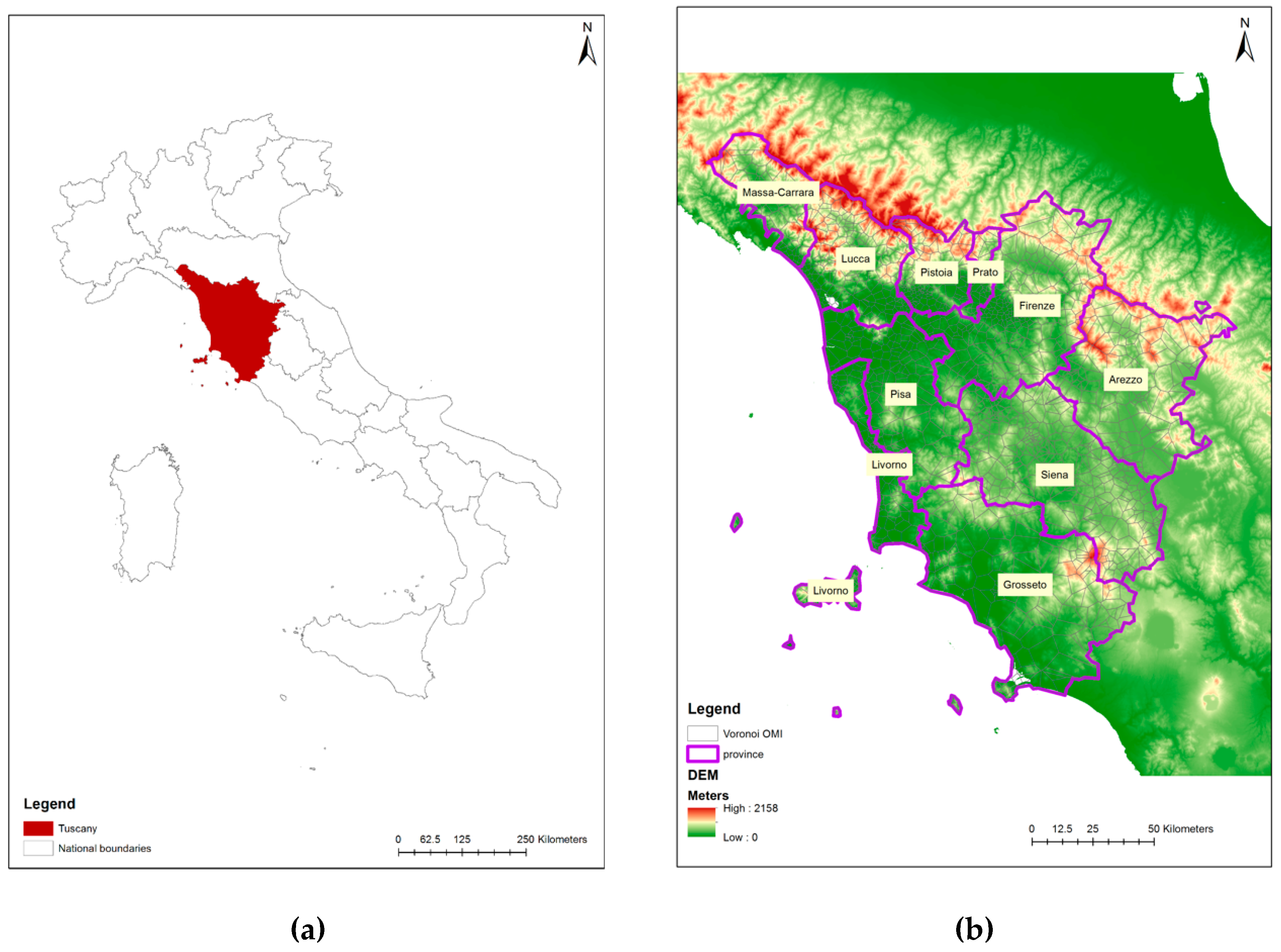
Considering the data available and the previous literature involved in real estate analysis, the work is focused on the following variables: (i) real estate values; (ii) distance from the inhabited centres; (iii) distance from roads; (iv) aesthetic values of the landscape. The analysis was performed in Tuscany, a region locates in the centre of Italy (Figure 1a,b).
There are several studies on spatial data analysis thanks to which local econometric techniques have been developed [25,26,27,28] to estimate local spatial associations [29]. Indeed, global indicator provides an indication of the spatial pattern of the phenomena without providing information for a particular local spatial unit. Therefore, Anselin [25] proposed the Local Indicator of Spatial Association (LISA), which identifies more effective spatial clustering by decomposing global spatial indicators to identify and test the areas that most contribute to them. Some examples are the LISA indicators, including local Moran’s I and local Geary’s c.
The global measure of autocorrelation Geary’s C [30] has the following expression:
where xi is the observed value of the population in location i, is the average of locations xi of n, W is the matrix of the spatial weightings wij (somewhat defined) between feature i and j, and n is equal to the total number of spatial features. The Geary’s C is greater than 1 if there is a negative spatial autocorrelation, equal to 1 in absence of spatial autocorrelation, and it is less than 1 if there is a positive spatial autocorrelation.
Anselin [25,31] first outlined and elaborated the local version of Geary statistic that uses a different measure of attribute similarity. It is focused on squared differences, or, rather, dissimilarity where small values of the statistics mean positive spatial autocorrelation, while large values mean negative spatial autocorrelation. Considering the local version of Geary C statistic, Equation (1) can be rewritten as follows.
where LGi is the Local Geary statistic at the location i-th, W is the matrix of the spatial weightings wij (somewhat defined) between locations i, and j and xi and xj are the observed value of the population in location i and j. This equation can be described as a weighted sum of the squared distance in attribute space for the geographical neighbours of i-th observation.
The positive local spatial autocorrelation is expressed by high-high, low-low, and other cases; the negative spatial autocorrelation Equation (2) indicates a large (larger than under spatial randomness) difference between neighbouring values, without suggesting a particular high-low or low-high pattern (due to the use of a squared difference as the criterion for attribute similarity, this distinction is not possible). Local Geary statistic can be extended in a multivariate way as proposed by Anselin [31], thus we can estimate spatial correlations simultaneously for several variables. A positive spatial autocorrelation means that the average distance in attribute space between the values at i-th location and the values at its neighbouring locations are smaller than what they would be under spatial randomness. If it is larger, we are in presence of negative spatial autocorrelation. It is important to note how the multivariate statistic is not simply the overlap of univariate statistics, so a univariate cluster could be not corresponding to a multivariate cluster. Indeed, the univariate statistics deal with distances in attribute space projected onto a single dimension, whereas the multivariate statistics are based on distances in a higher-dimensional space. The multivariate Local Geary formula is obtained by summing each Local Geary statistics of each variable examined:
where MLCn.i is the multivariate local Geary statistics of n variables at i-th location and LGv,i is the Local Geary statistic for variable v at location i. This measure corresponds to a weighted average of the squared distances in multidimensional attribute space between the values observed at a given geographic location i and those at its geographic neighbours.
In order to give a different interpretation of the spatial interaction between the observed variables, we provide the Spatial Durbin Model (SDM) [32,33,34,35], an extension of linear regression that considers both spatially endogenous interactions as well as exogenous spatial interactions. As argued by LeSage [36], Spatial Durbin Model is a spatial autoregressive model variant of the conventional model. SDM is written as follows:
where ρ is a scalar and is the autoregressive parameter that measures the spatial relationship between neighbours and the real estate price (reprice). The coefficient ρ is between zero, that means spatial independence, and one (spatial determined). βs are the parameters associated with road distance (roadd) and distance to city centres (citycenterd). θ is the spatial parameter of the esthetical values of landscape (esthval) of the neighbours. θ and ρ measure the spatial relation of the dependent variables. Therefore, the spatial pattern of real estate values is detected by the combination of the parameters ρ and θ. The first value measures the influence of neighbours’ real estate values while the second measures the influence of neighbours’ characteristics in terms of the esthetical values of the landscape. Again, W is the spatial weight matrix that contains a list of weights equal to wij. The spatial weight matrix is the same for both parameter and it is calculated as the inverse distance between areas. Finally, ε is the error term, normally distributed.
reprice = ρWreprice + β1roadd + β2citycenterd + θWesthval + ε
3. Analysis of Variables
3.1. Real Estate Values
There are several methods in the literature for establishing property values. Fan et al. [37] uses the decision tree approach to determine house prices in Singapore. The results show that buyers are predominantly interested in the intrinsic characteristics of homes such as the area, type, and age of the apartment. Jasinska and Preweda [38] use semiparametric models to analyse the spatial and temporal components of house prices. The same authors [39] combined quantitative statistical methods with qualitative and spatial characteristics to determine the cadastral value of the property of the city Bochnia.
In this work, we used the real estate values provided by the Real Estate Market Observatory (OMI), which estimates the real estate prices per homogeneous areas at provincial or municipal level different provinces and municipalities [40]. The OMI is a database that provides, for the whole national territory, the quotations of real estate values and leases every six months and is a relevant source of information and a useful tool for all market operators and scholars in the real estate sector, for public and private research institutes, and for the public administration.
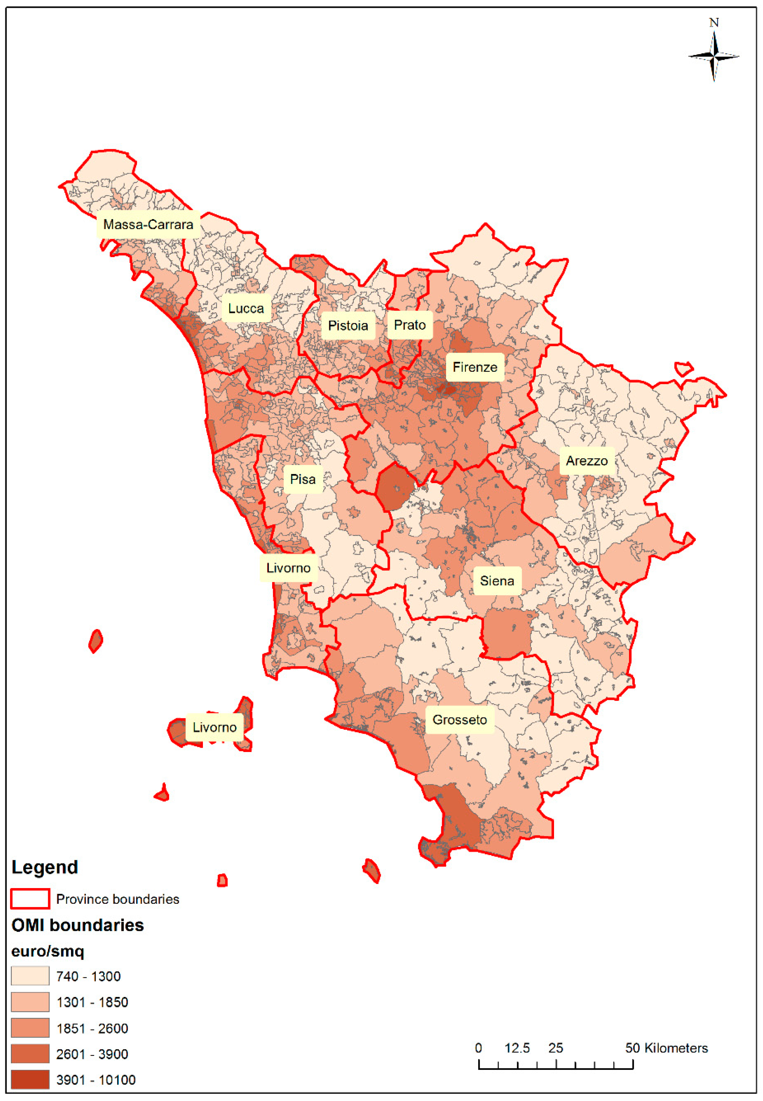
The six-monthly real estate quotations identify, for each delimited homogeneous territorial area (OMI zone) of each municipality, a minimum/maximum range per unit of area in euro per square meter. When for the same typology more than one state of conservation is valued, the prevailing one is however specified. The real estate quotations are divided into sections related to residential, commercial, tertiary, and production properties. For the analysis, we have based on the residential ones. The values of the second half of 2016 for civil housing have been considered, taking the maximum market value per square meter. These values range from a minimum of 740 euro/sqm in the town of Chiusdino (province of Siena) to a maximum of over 10,000 euro/sqm in the town of Forte dei Marmi (province of Lucca) while the average value in Tuscany is 1850 euro/sqm (Figure 2).
The spatial reference used in the analysis is EPSG projection 32,632-WGS 84/UTM zone 32 N.
3.2. Distance from the Inhabited Centres
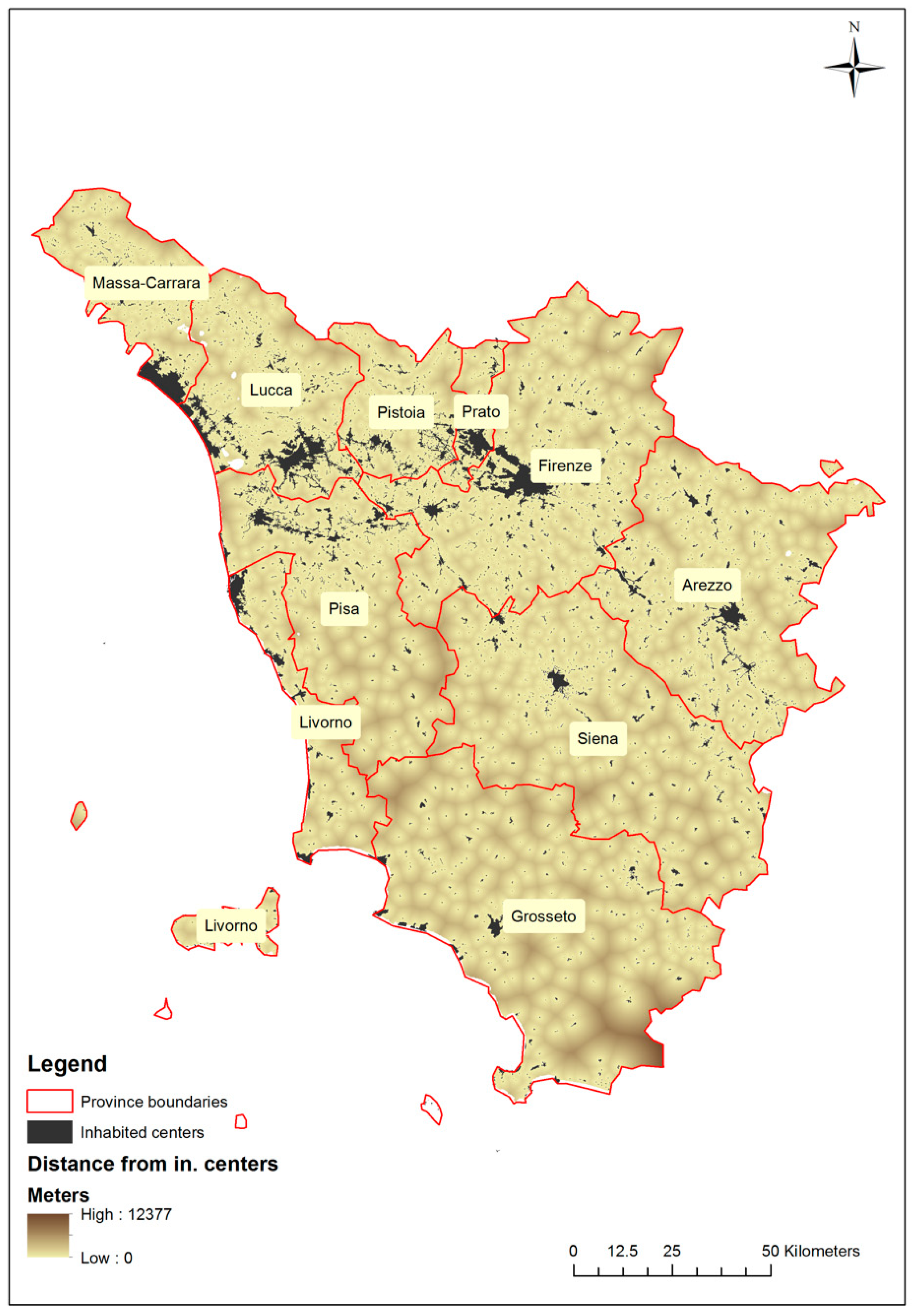
In literature, the distance from some features is widely adopted as a determinant of such values [41,42,43,44]. Specifically, the distance from inhabited areas is a widely adopted variable for real estate analysis [8]. The calculation of this variable was based on the map of the inhabited centre developed in 2003 by the Region of Tuscany. Starting from the polygon of the inhabited centre, a fuzzy distance has been calculated. As argued by Al-Ahmadi et al. [45], the fuzzy distance decay membership function is used to weigh the strength of the proximity to a given feature. Instead of having a single crisp threshold that denotes a distance from a feature, the fuzzy distance decay function can describe the absence of a service that increases with distance from inhabited centres. The values in Figure 3 represent the meters far from inhabited centres.
3.3. Distance from Roads
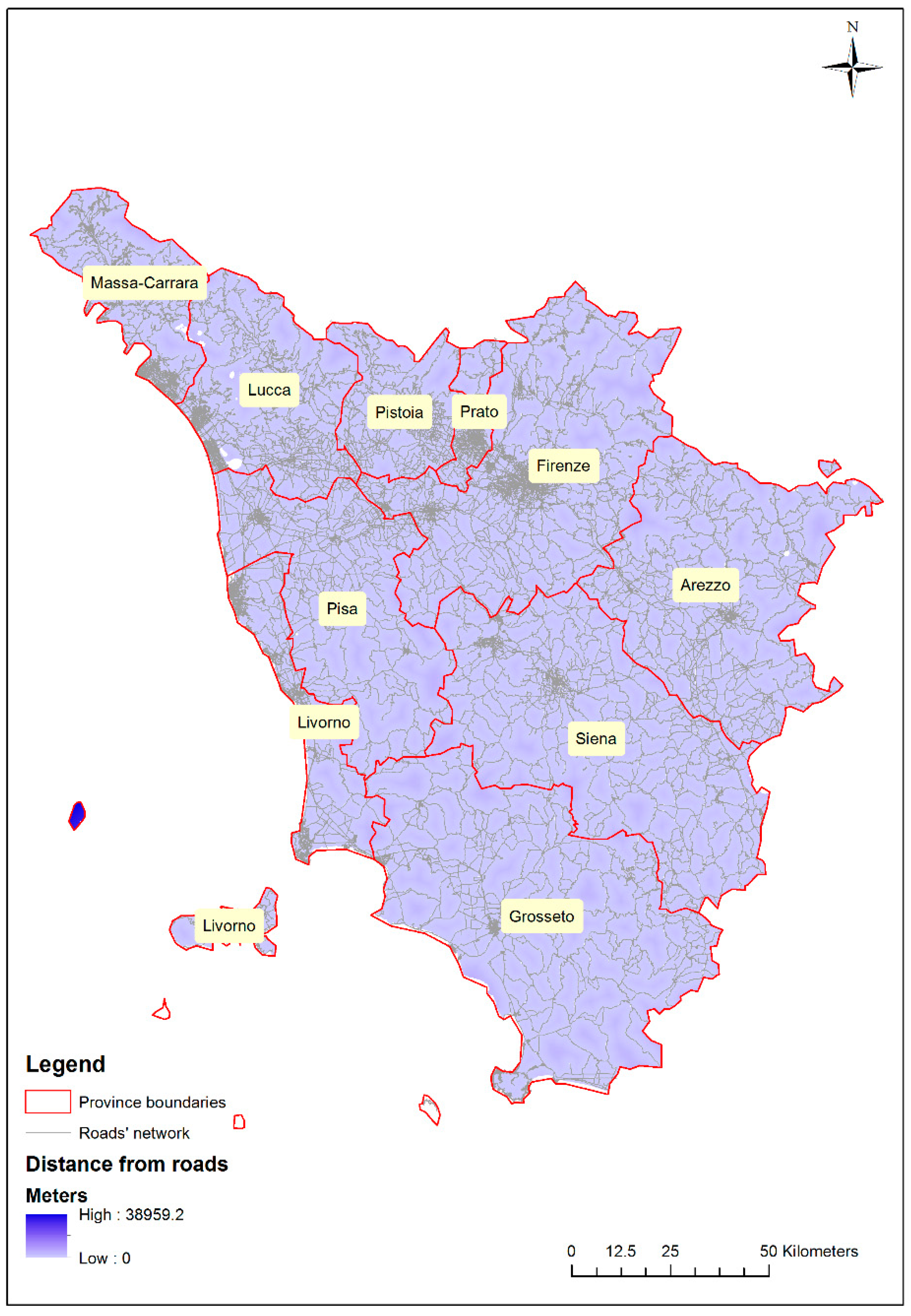
The study of the primary road network has been based on the “road traffic” maps developed in 2003 by the region of Tuscany. As the previous variable, starting from roads, a fuzzy distance has been calculated. It is possible to note how the entire region is characterized by a capillary road network that obviously increases in the proximity of inhabited centres. The interpretation of this variable is twofold: large distances from road network could mean both large distances from urban noises (positive aspects) and large distances from services (negative aspect). The values in Figure 4 represent the meters far from the road network.
3.4. Aesthetic Values of Landscape
The aesthetic value of landscape was carried out through a questionnaire promoted in the LIFE FutureForCoppiceS Project, LIFE14 ENV/IT/000514. Thanks to this project we tried to emphasize the importance of forest at different (economic, social, and environmental) levels [46,47,48,49,50,51,52,53]. Between July and September 2016, professional interviewers, through face-to-face interviews, made over 250 questionnaires to forest users in Tuscany. Participants were randomly selected in five forest districts of the project: the Caselli forests in the province of Pisa, the districts of Colline Metallifere and Alberese in the province of Grosseto, and the districts of Alpe di Catenaia and Alto Tevere in the province of Arezzo. We obtained 248 valid questionnaires composed of 54% of females and 46% of males; 66% of respondents have a high level of education (high school degree); 40% of the interviewed were 18–35 years old, and 27% were between 35 and 50 years old; 30% of the sample is composed of employed people and 29% were students. More statistics about respondents are described in previous works [54,55,56].
The three sections of questionnaires collected (i) information about respondents’ socio-demographic characteristics; (ii) the respondents’ aesthetic preferences related to landscape types; (iii) the willingness to pay for maintaining forests for recreational use under the management approaches. The third section was used in previous works [54,55,56], while we used the second section for the landscape analysis. The question was: “Can you express a liking rating for the agricultural and forestry landscape?” Using a five-point Likert scale ranging from 1 (less appreciated) to 5 (very appreciated), respondents provided information about their aesthetic evaluation of the following agricultural and forest landscapes: pasture, forest, and heterogeneous agricultural areas (temporary crops associated with permanent crops, cropping systems, and particle complex).
Areas are predominantly occupied by agricultural fields with significant natural areas and areas of agricultural woods). The forest received the highest rating with a percentage equal to 75% (4 and 5 on the Likert scale). Considering same values of Likert scale (4 and 5), the heterogeneous agricultural areas received a percentage equal to 48%, while the percentage of pasture was equal to 35%.
First, we calculated the aesthetic value for each landscape: for this purpose, we used the average value resulting from questionnaires. The average value of the Likert scale was previously used in another study [57]. This has been done considering that a Likert scale with five or more categories can often be used as continuous [58,59]. The aesthetic value of the forest was equal to 4.12, and the value of heterogeneous agricultural areas obtained was 3.46, while pasture received a value equal to 2.91.
4. Results and Discussion
For the analysis, an average distance from inhabited areas, road network, and average aesthetic value was attributed to each OMI area. OMI areas are disordered polygons with non-uniform perimeters—this could generate some problems with the spatial analysis (i.e., the spatial connection of features) that need well-defined figures in order to perform more accurate statistics.
To overcome this problem, OMI areas are transformed in Voronoi tessellation starting from the centroid of each area (1365 areas). As argued by Wang et al. [60] “Voronoi tessellation (VT) is a tool to divide 2D/3D space into convex polygons/polyhedrons without overlaps or gaps based on a group of points or objects in the space. No matter how disordered the discrete points are distributed in the space, VT can strictly divide the “local space” around each point, so that a number of “neighbours” can always be identified uniquely based on the connections of these local spaces.” This is very useful in the methods that rely on the relationships between a feature and its neighbours [61,62].
According to this transformation of OMI polygons in Voronoi tessellation, it is possible to notice how the highest real estate values are referred to the coastal area (especially in the southern part of Tuscany, the province of Grosseto) and in the proximity of the big cities. If we consider the distance from urban centres and roads, the highest average values are in the southern part of the province of Pisa and in the mountainous areas of the Apennines. As far as landscape values are concerned, the highest average values are recorded in the mountainous areas in the central part of the province of Pisa and in the southern part of the province of Grosseto (see maps in Section 1 of the Supplementary Materials).
Considering that in the spatial autocorrelation statistic the indicator for geographical or locational similarity is expressed in the form of spatial weights (wij); we calculated them with inverse distance weight. Therefore, the spillover effects are greater for the closest areas and negligible for the distant ones.
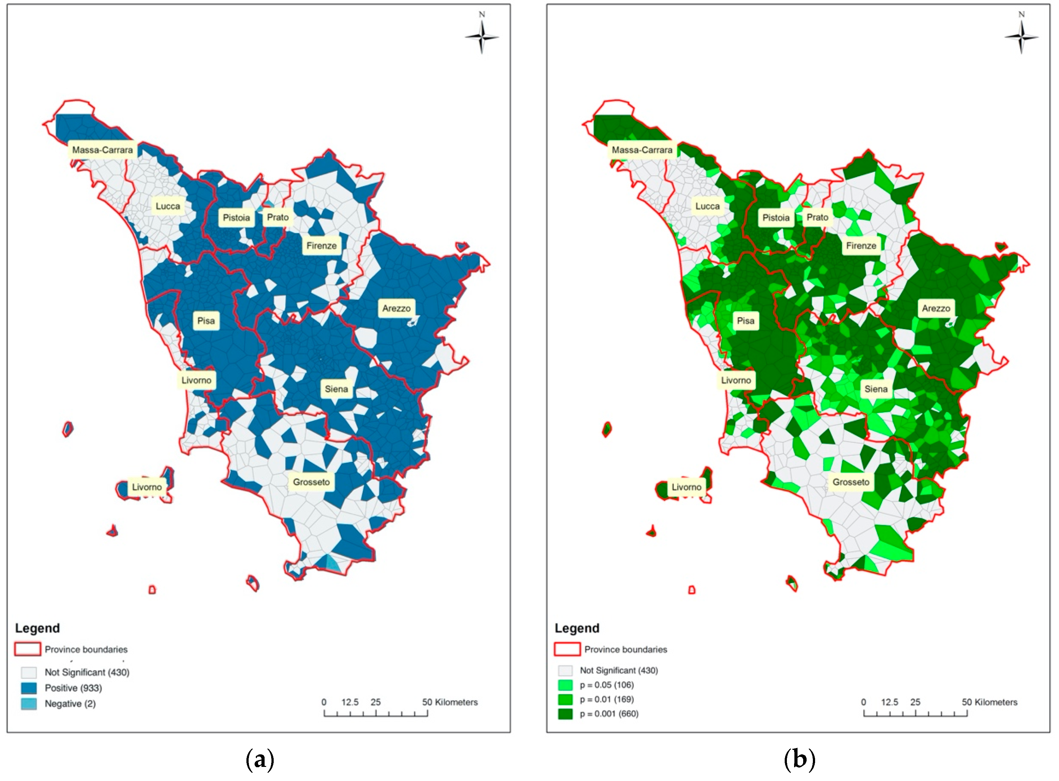
Figure 6a shows the clusters obtained from the Multivariate Local Geary analysis. There are positive clusters in the central and north-western part of the region and negative clusters in the southern part of the region. Considering the significance of the clusters (Figure 6b), the strongest correlations (p-value = 0.001) are concentrated around the metropolitan areas of Florence and Pisa.
Other significant clusters (p = 0.01) are located in the northwest part of the region including the provinces of Pistoia, Lucca, Massa Carrara, and the mountainous area of the Tosco-Emiliano Apennine. Considering a significance of p = 0.05, the significant clusters are located in the provinces of Arezzo (including the mountainous area of the Tosco-Romagnolo Apennine), Siena, and in the southern part of the region belonging to the province of Grosseto.
To better understand the results, it is useful to also consider the clusters of each variable obtained through a Univariate Local Geary analysis (see maps in Section 2 of the Supplementary Materials).
Considering the OMI values, it is possible to highlight high correlations (which means high real estate values) that cover the municipalities of Florence, Siena, Pisa, and the neighbouring municipalities and the entire coastal part of Tuscany. These values correspond to clusters with low values of landscape and low distances from urban centres and roads. This is justified by the fact that the high real estate values are inserted in anthropized contexts close to roads and urban centres where the landscape does not have a high value.
Vice versa clusters with low real estate values are found in areas opposite to the previous ones that are represented by the mountain areas along the Apennine chain, with high landscape values due to the strong presence of forests and high distances from urban centres and roads (especially near the mountain areas of the Tosco-Emiliano Apennine). These results are in line with some works in literature [4,7,8] in which real estate values are strongly influenced by the proximity to services. It is important to examine in more detail these last two variables because it is widely studied in our country from a different point of view [63,64,65,66]. Distances from urban centres and roads show both clusters with high values (areas far from urban centres and roads at the same time) in the area of the province of Pisa (excluding the urban area of Pisa town). In this area, the real estate prices are low—this is due to the presence of a coastal area that is much more attractive in terms of tourism and therefore in terms of real estate prices. Indeed, this area is much less frequented by people despite the presence of a protected area with a high degree of biodiversity such as the Merse Valley [42] and many other naturalistic areas (i.e Monterufoli-Caselli forests, Montefalcone natural reserve, and Cerbaie a Natura 2000 Site of Community Importance).
These results lead us to conclude how, despite how forested areas are more appreciated than other landscapes, they have a low influence on the prices of houses located in those areas which are essentially related to the parameters related to the proximity to services.
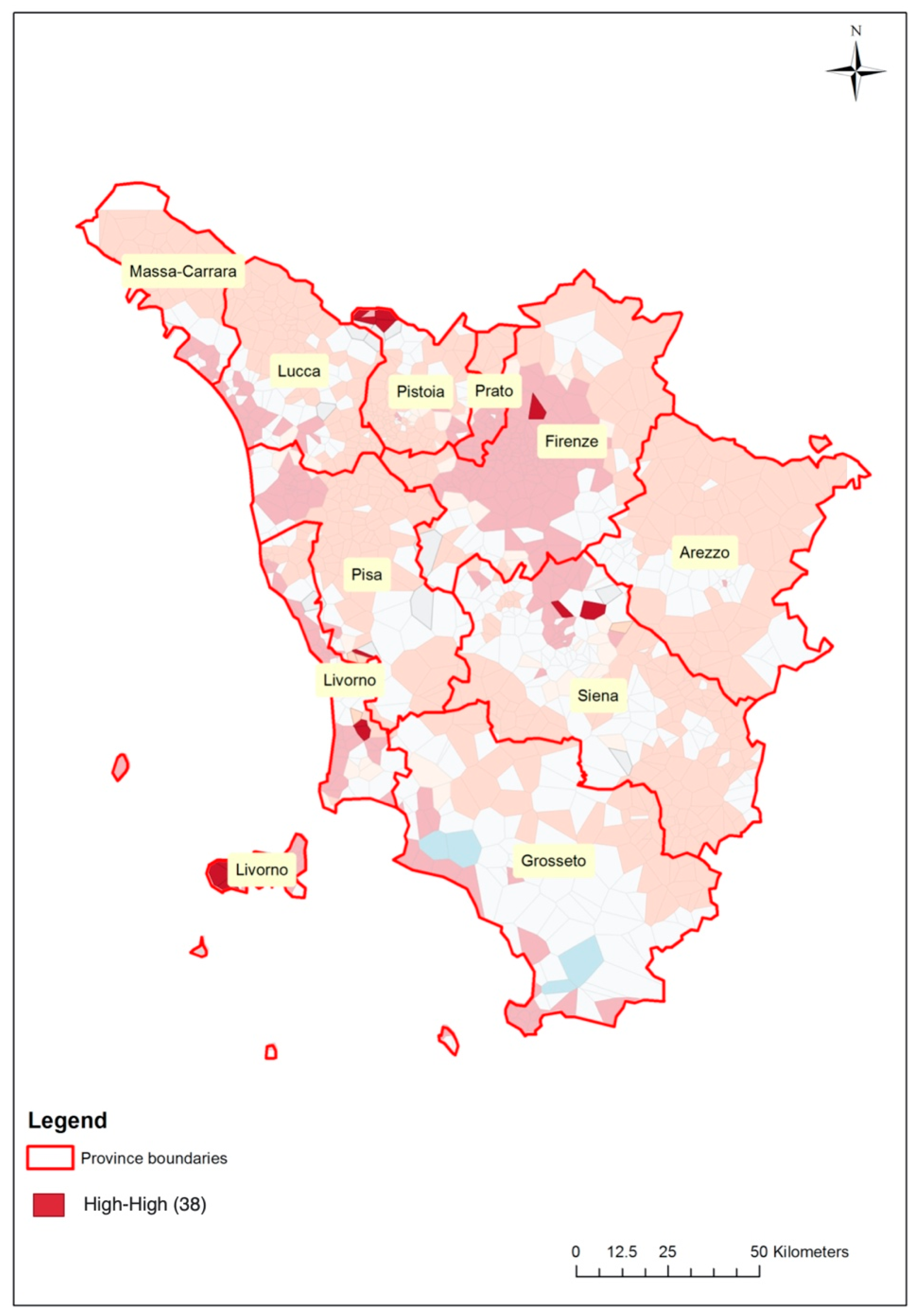
However, there are some areas with opposite values compared to previous ones: in these areas high real estate values are linked to high landscape values, and average high distances from services (Figure 7). These data in countertrend could be explained as follows.
One cluster is located in Abetone Cutigliano municipality (province of Pistoia) which is characterized by the presence of the most famous ski area of the region. This could justify the high real estate values in forested areas far from services offered by cities. Another cluster is related to the Chianti Senese (province of Siena) where real estate values are affected by the surrounded territory particularly suited to the production of the Chianti wine famous throughout the world.
The last cluster is related to the Bolgheri area (province of Livorno), where the Naturalistic Oasis of Bolgheri is located. The high values of real estate could be justified by the strategic position of the area close to the seaside. Moreover, this location is very famous in Italy due to the famous vineyards and the poetry “Davanti San Guido” by Giosuè Carducci (1906 Nobel Prize in literature) who praised the landscape beauty of this area.
Adopting this interpretation of the results, we need to consider some aspects regarding multivariate statistics adopted.
Despite the fact that Multivariate Local Geary statistic could be described as the combination of attribute similarity and locational similarity and its application is the sum of the univariate local statistics for each variable, it involves different trade-offs.
Generally speaking, it is the average squared distance in multivariate attribute space between a certain point and its geographic neighbours (as defined by a spatial weights matrix). So, considering a multivariate scenario, the clusters obtained can differ from the simple overlay of univariate statistics.
The multivariate analysis can lead to spatial aggregations that are not explained in its univariate counterparts. Indeed, “the multivariate measure of attribute similarity is not a simple extrapolation of the univariate measures, but it involves complex trade-offs in all attribute dimensions considered. Multivariate statistics focus on a combination of the distances along the different variable dimensions, rather than taking each as being orthogonal” [31]. In fact, the change analysis from univariate statistics to a multivariate context is still a new frontier in spatial autocorrelation.
In a second step, the relationships between the observed variables have been analysed differently through the Spatial Durbin Model (Table 2). The parameter ρ is significant and positive. This demonstrates that an ordinary least-squares estimate would be biased.
As suggested by Lacombe and LeSage [67] and LeSage [36], to measure the different impacts of changes in an explanatory variable, it is possible to use scalar summary measures decomposing results in the summary measures of direct, indirect, and total impacts (Table 3). The direct impact measures the effect of the independent variables of i-th polygon on the dependent variable of the same polygon. The indirect one measures the effect on the dependent variable of i-th polygon of the independent variables belonging to the neighbouring polygons. The total effect represents the sum of the previous effects [36,67].
The direct effect of aesthetic values was not significantly different from zero. This means that the aesthetical values of the landscapes will have no effect on real estate values, while both the distance from urban centres with a negative sign and the distance to roads have a significant direct impact on it. Therefore, real estate distant to cities has, as expected, lowered price while real estate distant to roads has a higher price. In contrast, the indirect impacts of explanatory variables belonging to nearby polygons were all significant with the opposite sign for the variables distance to centres and distance to roads. This suggests that increased distance aesthetical value of the neighbouring area has a positive impact on real estate price; thus, the total effect is due exclusively by the indirect effect.
5. Conclusions
The study of the correlation between the real estate values and the territory has started using two variables (of proximity to the services) consolidated in literature and a third experimental variable constituted by the landscape values. The aim was to investigate the spatial relationships between the analysed data. T hypothesis of a spatial relationship of the data identifying the consistent relationship between variables, both in terms of geographical space and data space, has been tested. This work could represent a useful tool for decision-makers to planning territorial strategies considering the social, economic, and environmental aspects. Indeed, thanks to this spatial analysis, the policymakers could be assisted to help people to search for housing based on the services/characteristics of different geographical areas. Our results could also be used to analyse how the real estate situation is directly or indirectly related to the quality of life of citizens.
Another use of our research could be related to better understand the development of the tourism landscape: this an important aspect because, as argued Chen et al. [6] “it can lead its peripheral land price and the real estate price to rise well, and then promote the development of peripheral real estate industry. Under these effects, various cities, according to own comparative superiority, develop own city tourist resources, constructs typical landscape engineering, guides the property developer to develop peripheral land of the scenic area reasonably, strengthens the protection and the development of the ecological environment and the humanities resources, makes the tourist and the inhabitant glad to sightsee or live, makes it to be the driving force for the city real estate industry in order to lead the urban economy to develop."
As a final remark, it is important to keep in mind that these types of investigations are possible thanks to the rapid improvement of geospatial data collection techniques and the availability of a large amount of geospatial data [68].
Our findings demonstrate a significant spatial dependence in the real estate prices highlighted by the significant and positive Rho coefficient in the spatial Durbin model. This implies that extrinsic features play a crucial role in determining house price and that there are spatial spillovers. Specifically, the aesthetic values influence the real estate price throughout in more of a spatial indirect effect rather than the direct effect. This means that when buying homes, individuals prefer other aspects such as proximity to essential services. Indeed, the results seem to show that people prefer to live inside well-served areas, and at the same time, nearby areas with high aesthetic values. The results relating to the distance from the main roads, however, seem counterintuitive. This result probably depends on the evidence that these areas suffer from greater traffic jam or pollution or they are preferred for alternative uses such as for locating industrial plants or big shopping centres rather than residential use. Therefore, these effects decrease house prices.
Clearly, this study has some limitations. A first limitation is to consider the average value of an area (OMI area) and not of a specific type of house. This was necessary given the wide territory of analysis (an entire region), but we do not have values with high scale detail, so it is difficult to find similar studies with which to compare our results. The real estate values used are not very detailed. We used OMI area with maximum and minimum values sort by types of building, with low details regarding the property intrinsic attributes. Moreover, this type of analysis is related to the availability of georeferenced databases that are often difficult to acquire. For the calculation of landscape values, other parameters should be considered, such as slope, exposure, tree essence, etc., but this should comprise a separate work.
Our work, made at a regional scale, could give general indications, highlighting possible critical points or outlining lines of intervention for stakeholders. Clearly, it must be accompanied by more specific studies in the areas to deepen and better interpret the general indications mentioned above.
Supplementary Materials
The following are available online at https://0-www-mdpi-com.brum.beds.ac.uk/2071-1050/13/4/2236/s1, Figure S1: OMI values attributed to Voronoi tessellations, Figure S2: Average distances from urban centre attributed to Voronoi tessellations, Figure S3: Average distances from roads attributed to Voronoi tessellations, Figure S4: Average aesthetic values attributed to Voronoi tessellations, Figure S5: OMI values cluster map, Figure S6: Distance from inhabited centre cluster map, Figure S7: Distance from roads cluster map, Figure S8: Aesthetic values cluster map.
Author Contributions
F.R.: conceptualization, methodology, software, writing—original draft preparation, writing—reviewing and editing, supervision. R.F.: reviewing and editing. F.B.: conceptualization, methodology, software, writing—reviewing and editing, validation. All authors have read and agreed to the published version of the manuscript.
Funding
This research was funded by the LIFE Programme of the European Commission, under the Grant Agreement LIFE14 ENV/IT/000514 (LIFE FutureForCoppiceS, “Shaping future forestry for sustainable coppices in Southern Europe: the legacy of past management trials”).
Institutional Review Board Statement
Not applicable.
Informed Consent Statement
Informed consent was obtained from all subjects involved in the study.
Data Availability Statement
Data are available on request.
Conflicts of Interest
The authors declare no conflict of interest.
References
- Jim, C.Y.; Chen, W.Y. Value of scenic views: Hedonic assessment of private housing in Hong Kong. Landsc. Urban Plan. 2009, 91, 226–234. [Google Scholar] [CrossRef]
- Damigos, D.; Anyfantis, F. The value of view through the eyes of real estate experts: A Fuzzy Delphi Approach. Landsc. Urban Plan. 2011, 101, 171–178. [Google Scholar] [CrossRef]
- Cervero, R.; Kang, C.D. Bus rapid transit impacts on land uses and land values in Seoul, Korea. Transp. Policy 2011, 18, 102–116. [Google Scholar] [CrossRef] [Green Version]
- Ibeas, Á.; Cordera, R.; Dell’Olio, L.; Coppola, P.; Dominguez, A. Modelling transport and real-estate values interactions in urban systems. J. Transp. Geogr. 2012, 24, 370–382. [Google Scholar] [CrossRef] [Green Version]
- Rodríguez, D.A.; Mojica, C.H. Capitalization of BRT network expansions effects into prices of non-expansion areas. Transp. Res. Part A Policy Pract. 2009, 43, 560–571. [Google Scholar] [CrossRef]
- Chen, A.; Han, Y.; Tan, X. Analysis of Tourism and Landscape Engineering on Real Estate Impact Based on Correlation. Syst. Eng. Procedia 2011, 1, 286–293. [Google Scholar] [CrossRef] [Green Version]
- Voith, R. Transportation, Sorting and House Values. Real Estate Econ. 1991, 19, 117–137. [Google Scholar] [CrossRef]
- D’Acci, L. Quality of urban area, distance from city centre, and housing value. Case study on real estate values in Turin. Cities 2019, 91, 71–92. [Google Scholar] [CrossRef]
- Mathur, S. Impact of transit stations on house prices across entire price spectrum: A quantile regression approach. Land Use Policy 2020, 99, 104828. [Google Scholar] [CrossRef]
- Luttik, J. The value of trees, water and open space as reflected by house prices in the Netherlands. Landsc. Urban Plan. 2000, 48, 161–167. [Google Scholar] [CrossRef]
- Kong, F.; Yin, H.; Nakagoshi, N. Using GIS and landscape metrics in the hedonic price modeling of the amenity value of urban green space: A case study in Jinan City, China. Landsc. Urban Plan. 2007, 79, 240–252. [Google Scholar] [CrossRef]
- Kumagai, Y.; Yamada, Y. Green space relations with residential values in downtown Tokyo—Implications for urban biodiversity conservation. Local Environ. 2008, 13, 141–157. [Google Scholar] [CrossRef]
- Joly, D.; Brossard, T.; Cavailhès, J.; Hilal, M.; Tourneux, F.-P.; Tritz, C.; Wavresky, P. A Quantitative Approach to the Visual Evaluation of Landscape. Ann. Assoc. Am. Geogr. 2009, 99, 292–308. [Google Scholar] [CrossRef]
- Donovan, G.H.; Butry, D.T. Trees in the city: Valuing street trees in Portland, Oregon. Landsc. Urban Plan. 2010, 94, 77–83. [Google Scholar] [CrossRef]
- Donovan, G.H.; Landry, S.; Winter, C. Urban trees, house price, and redevelopment pressure in Tampa, Florida. Urban For. Urban Green. 2019, 38, 330–336. [Google Scholar] [CrossRef]
- Li, W.; Saphores, J.-D. A Spatial Hedonic Analysis of the Value of Urban Land Cover in the Multifamily Housing Market in Los Angeles, CA. Urban Stud. 2012, 49, 2597–2615. [Google Scholar] [CrossRef]
- Glaesener, M.L.; Caruso, G. Neighborhood green and services diversity effects on land prices: Evidence from a multilevel hedonic analysis in Luxembourg. Landsc. Urban Plan. 2015, 143, 100–111. [Google Scholar] [CrossRef]
- Trojanek, R.; Gluszak, M.; Tanas, J. The effect of urban green spaces on house prices in Warsaw. Int. J. Strat. Prop. Manag. 2018, 22, 358–371. [Google Scholar] [CrossRef]
- Troy, A.; Grove, J.M. Property values, parks, and crime: A hedonic analysis in Baltimore, MD. Landsc. Urban Plan. 2008, 87, 233–245. [Google Scholar] [CrossRef]
- Tajima, K. New Estimates of the Demand for Urban Green Space: Implications for Valuing the Environmental Benefits of Boston’s Big Dig Project. J. Urban Aff. 2003, 25, 641–655. [Google Scholar] [CrossRef]
- Crompton, J. Parks and Economic Development; APA Planning Advisory Service, Ed.; APA Planning Advisory Service: Chicago, IL, USA, 2001. [Google Scholar]
- Benjamin, J.D.; Sirmans, G.S. Mass Transportation, Apartment Rent and Property Values. J. Real Estate Res. 1996, 12, 1–8. [Google Scholar]
- Debrezion, G.; Pels, E.; Rietveld, P. The impact of railway stations on residential and commercial property value: A meta-analysis. J. Real Estate Financ. Econ. 2007, 35, 161–180. [Google Scholar] [CrossRef] [Green Version]
- D’Acci, L. Monetary, subjective and quantitative approaches to assess urban quality of life and pleasantness in cities (Hedonic Price, Willingness-to-pay, Positional Value, life satisfaction, Isobenefit lines). Soc. Indic. Res. 2014, 115, 531–559. [Google Scholar] [CrossRef] [Green Version]
- Anselin, L. Local Indicators of Spatial Association—LISA. Geogr. Anal. 1995, 27, 93–115. [Google Scholar] [CrossRef]
- Boots, B. Developing local measures of spatial association for categorical data. J. Geogr. Syst. 2003, 5, 139–160. [Google Scholar] [CrossRef]
- Fotheringham, A.S.; Brunsdon, C. Local Forms of Spatial Analysis. Geogr. Anal. 2010, 31, 340–358. [Google Scholar] [CrossRef]
- Boncinelli, F.; Bartolini, F.; Casini, L.; Brunori, G. On farm non-agricultural activities: Geographical determinants of diversification and intensification strategy. Lett. Spat. Resour. Sci. 2017, 10, 17–29. [Google Scholar] [CrossRef]
- Lloyd, C. Local Models for Spatial Analysis; Routledge: London, UK, 2010. [Google Scholar]
- Geary, R.C. The Contiguity Ratio and Statistical Mapping. Inc. Stat. 1954, 5, 115. [Google Scholar] [CrossRef]
- Anselin, L. A Local Indicator of Multivariate Spatial Association: Extending Geary’s c. Geogr. Anal. 2019, 51, 133–150. [Google Scholar] [CrossRef]
- Basile, R.; Mínguez, R. Advances in spatial econometrics: Parametric vs. Semiparametric spatial autoregressive models. In Springer Proceedings in Complexity; Springer: Berlin/Heidelberg, Germany, 2018; pp. 81–106. [Google Scholar]
- Zhu, Y.; Han, X.; Chen, Y. Bayesian estimation and model selection of threshold spatial Durbin model. Econ. Lett. 2020, 188, 108956. [Google Scholar] [CrossRef]
- Feng, Y.; Wang, X. Effects of urban sprawl on haze pollution in China based on dynamic spatial Durbin model during 2003–2016. J. Clean. Prod. 2020, 242, 118368. [Google Scholar] [CrossRef]
- Boncinelli, F.; Riccioli, F.; Casini, L. Spatial structure of organic viticulture: Evidence from Chianti (Italy). New Medit J. 2017, 16, 55–63. [Google Scholar]
- LeSage, J.P. Introduction to Spatial Econometrics; Chapman and Hall: London, UK, 2008. [Google Scholar]
- Fan, G.-Z.; Ong, S.E.; Koh, H.C. Determinants of House Price: A Decision Tree Approach. Urban Stud. 2006, 43, 2301–2315. [Google Scholar] [CrossRef]
- Jasinska, E.; Preweda, E. The use of regression trees to the analysis of real estate market of housing. In Proceedings of the International Multidisciplinary Scientific GeoConference Surveying Geology and Mining Ecology Management, SGEM, Albena, Bulgaria, 16–22 June 2013; Volume 2, pp. 503–508. [Google Scholar]
- Jasińska, E.; Preweda, E. Determining the cadastral-tax areas for the real estate premises based on the model of qualitative and quantitative. In Proceedings of the Environmental Engineering, Vilnius, Lithuania, 27–28 April 2017. [Google Scholar]
- OMI Manuale della Banca Dati Quotazioni. 2018. Available online: https://www.agenziaentrate.gov.it/portale/web/guest/schede/fabbricatiterreni/omi/manuali-e-guide (accessed on 18 February 2021).
- Malczewski, J. GIS-based land-use suitability analysis: A critical overview. Prog. Plann. 2004, 62, 3–65. [Google Scholar] [CrossRef]
- Riccioli, F.; Fratini, R.; Boncinelli, F.; El Asmar, T.; El Asmar, J.-P.J.P.; Casini, L. Spatial analysis of selected biodiversity features in protected areas: A case study in Tuscany region. Land Use Policy 2016, 57, 540–554. [Google Scholar] [CrossRef]
- Riccioli, F.; Boncinelli, F.; Fratini, R.; El Asmar, J.; Casini, L. Geographical Relationship between Ungulates, Human Pressure and Territory. Appl. Spat. Anal. Policy 2019, 12, 847–870. [Google Scholar] [CrossRef]
- Feng, Y.; Liu, Y. Scenario prediction of emerging coastal city using CA modeling under different environmental conditions: A case study of Lingang New City, China. Environ. Monit. Assess. 2016, 188, 1–15. [Google Scholar] [CrossRef]
- Al-Ahmadi, K.; See, L.; Heppenstall, A.; Hogg, J. Calibration of a fuzzy cellular automata model of urban dynamics in Saudi Arabia. Ecol. Complex. 2009, 6, 80–101. [Google Scholar] [CrossRef]
- Loomis, J.B. Updated Outdoor Recreation Use Values on National Forests and Other Public Lands; US Department of Agriculture, Forest Service, Pacific Northwest Research Station: Corvallis, OR, USA, 2005.
- Zandersen, M.; Tol, R.S.J. A meta-analysis of forest recreation values in Europe. J. For. Econ. 2009, 15, 109–130. [Google Scholar] [CrossRef]
- Voces González, R.; Díaz Balteiro, L.; López-Peredo Martínez, E. Spatial valuation of recreation activities in forest systems: Application to province of Segovia (Spain). For. Syst. 2010, 19, 36. [Google Scholar] [CrossRef] [Green Version]
- Boncinelli, F.; Riccioli, F.; Marone, E. Do forests help to keep my body mass index low? For. Policy Econ. 2015, 54, 11–17. [Google Scholar] [CrossRef]
- Grima, N.; Singh, S.J.; Smetschka, B. Improving payments for ecosystem services (PES) outcomes through the use of Multi-Criteria Evaluation (MCE) and the software OPTamos. Ecosyst. Serv. 2018, 29, 47–55. [Google Scholar] [CrossRef]
- Aza, A.; Riccioli, F.; Di Iacovo, F. Optimising payment for environmental services schemes by integrating strategies: The case of the Atlantic Forest, Brazil. For. Policy Econ. 2021, 125, 102410. [Google Scholar] [CrossRef]
- Merlo, M.; Croitoru, L. Valuing Mediterranean Forests: Towards Total Economic Value; Merlo, M., Croitoru, L., Eds.; CABI: Wallingford, UK, 2005; ISBN 9780851999975. [Google Scholar]
- Pearce, D.W. The Economic Value of Forest Ecosystems. Ecosyst. Health 2001, 7, 284–296. [Google Scholar] [CrossRef]
- Riccioli, F.; Marone, E.; Boncinelli, F.; Tattoni, C.; Rocchini, D.; Fratini, R. The recreational value of forests under different management systems. New For. 2019, 50, 345–360. [Google Scholar] [CrossRef] [Green Version]
- Riccioli, F.; Fratini, R.; Marone, E.; Fagarazzi, C.; Calderisi, M.; Brunialti, G. Indicators of sustainable forest management to evaluate the socio-economic functions of coppice in Tuscany, Italy. Socioecon. Plan. Sci. 2019, 70, 100732. [Google Scholar] [CrossRef]
- Riccioli, F.; Fratini, R.; Fagarazzi, C.; Cozzi, M.; Viccaro, M.; Romano, S.; Rocchini, D.; Espinosa Diaz, S.; Tattoni, C. Mapping the Recreational Value of Coppices’ Management Systems in Tuscany. Sustainability 2020, 12, 8039. [Google Scholar] [CrossRef]
- Othman, N.; Mohamed, N.; Ariffin, M.H. Landscape Aesthetic Values and Visiting Performance in Natural Outdoor Environment. Procedia-Soc. Behav. Sci. 2015, 202, 330–339. [Google Scholar] [CrossRef] [Green Version]
- Sullivan, G.M.; Artino, A.R. Analyzing and Interpreting Data from Likert-Type Scales. J. Grad. Med. Educ. 2013, 5, 541–542. [Google Scholar] [CrossRef] [PubMed] [Green Version]
- Norman, G. Likert scales, levels of measurement and the “laws” of statistics. Adv. Health Sci. Educ. 2010, 15, 625–632. [Google Scholar] [CrossRef]
- Wang, S.; Tian, Z.; Dong, K.; Xie, Q. Inconsistency of neighborhood based on Voronoi tessellation and Euclidean distance. J. Alloys Compd. 2021, 854, 156983. [Google Scholar] [CrossRef]
- Jones, T.R.; Carpenter, A.; Golland, P. Voronoi-based segmentation of cells on image manifolds. In Proceedings of the Lecture Notes in Computer Science (Including Subseries Lecture Notes in Artificial Intelligence and Lecture Notes in Bioinformatics), Beijing, China, 21 October 2005; Springer: Berlin/Heidelberg, Germany, 2005; Volume 3765, pp. 535–543. [Google Scholar]
- Ushizima, D.M.; Bianchi, A.G.C.; Carneiro, C.M. Segmentation of Subcellular Compartments Combining Superpixel Representation with Voronoi Diagrams; Lawrence Berkeley National Lab (LBNL): Berkeley, CA, USA, 2015.
- Orsi, F.; Scuttari, A.; Marcher, A. How much traffic is too much? Finding the right vehicle quota for a scenic mountain road in the Italian Alps. Case Stud. Transp. Policy 2020, 8, 1270–1284. [Google Scholar] [CrossRef]
- Beria, P.; Debernardi, A.; Ferrara, E. Measuring the long-distance accessibility of Italian cities. J. Transp. Geogr. 2017, 62, 66–79. [Google Scholar] [CrossRef]
- De Matteis, F.; Preite, D.; Striani, F.; Borgonovi, E. Cities’ role in environmental sustainability policy: The Italian experience. Cities 2020, in press. [Google Scholar] [CrossRef]
- Boncinelli, F.; Pagnotta, G.; Riccioli, F.; Casini, L. The Determinants of Quality of Life in Rural Areas From a Geographic Perspective: The Case of Tuscany. Rev. Urban Reg. Dev. Stud. 2015, 27, 104–117. [Google Scholar] [CrossRef]
- Lacombe, D.J.; LeSage, J.P. Use and interpretation of spatial autoregressive probit models. Ann. Reg. Sci. 2018, 60, 1–24. [Google Scholar] [CrossRef]
- Shekhar, S.; Xiong, H.; Zhou, X. Encyclopedia of GIS; Springer: Berlin/Heidelberg, Germany, 2017. [Google Scholar]
Figure 1.
The analysis was performed in Tuscany, a region of center Italy (a) that is mainly hilly with mountain chains (called Apennines) located in the north part of the region (b).
Figure 1.
The analysis was performed in Tuscany, a region of center Italy (a) that is mainly hilly with mountain chains (called Apennines) located in the north part of the region (b).

Figure 2.
Real Estate Market Observatory (OMI) areas.

Figure 3.
Distance from inhabited centres.

Figure 4.
Distance from roads.

Figure 5.
Aesthetic value sort by land use.

Figure 6.
Multivariate Local Geary cluster map based on the transformation of OMI areas in Voronoi polygons (a) and the significance map related to Multivariate Local Geary cluster map (b).
Figure 6.
Multivariate Local Geary cluster map based on the transformation of OMI areas in Voronoi polygons (a) and the significance map related to Multivariate Local Geary cluster map (b).

Figure 7.
Cluster areas with high values of real estate, distance from inhabited centres, distance from roads and aesthetic values.
Figure 7.
Cluster areas with high values of real estate, distance from inhabited centres, distance from roads and aesthetic values.


Table 1.
Aesthetic values.
| Landscape | Corine Land Cover (CLC) Code | Aesthetic Value |
|---|---|---|
| Pasture | 230–240 | 2.91 |
| Heterogeneous agricultural areas | 210–229, 241–300 | 3.46 |
| Forest | 300–400 | 4.12 |
Table 2.
Spatial Durbin statistics.
| Real Estate | Coef. | Std. Err. | z | P > |z| |
|---|---|---|---|---|
| Aesthetical value | 7.30 | 19.76 | 0.37 | 0.712 |
| Distance to Centres | –0.25 | 0.04 | –6.29 | 0.000 |
| Distance to Roads | 0.07 | 0.02 | 3.01 | 0.003 |
| Constant | 2730.32 | 92.28 | 29.59 | 0.000 |
| W·Aesthetical values | –2123.76 | 60.90 | –34.87 | 0.000 |
| ρ·W·reprice | 2.45 | 0.07 | 37.36 | 0.000 |
Table 3.
Effects of estimation.
| Direct | dy/dx | Std. Err. | z | P > |z| |
|---|---|---|---|---|
| Aesthetical value | 13.30 | 18.39 | 0.720 | 0.470 |
| Distance to Centres | –0.25 | 0.04 | –6.290 | 0.000 |
| Distance to Roads | 0.07 | 0.02 | 3.010 | 0.003 |
| Indirect | ||||
| Aesthetical value | 1411.61 | 209.27 | 6.750 | 0.000 |
| Distance to Centres | 0.41 | 0.09 | 4.720 | 0.000 |
| Distance to Roads | –0.11 | 0.04 | –2.780 | 0.005 |
| Total | ||||
| Aesthetical value | 1424.90 | 206.69 | 6.890 | 0.000 |
| Distance to Centres | 0.16 | 0.06 | 2.550 | 0.011 |
| Distance to Roads | -0.04 | 0.02 | –2.060 | 0.040 |
Publisher’s Note: MDPI stays neutral with regard to jurisdictional claims in published maps and institutional affiliations. |
© 2021 by the authors. Licensee MDPI, Basel, Switzerland. This article is an open access article distributed under the terms and conditions of the Creative Commons Attribution (CC BY) license (http://creativecommons.org/licenses/by/4.0/).
Share and Cite
MDPI and ACS Style
Riccioli, F.; Fratini, R.; Boncinelli, F. The Impacts in Real Estate of Landscape Values: Evidence from Tuscany (Italy). Sustainability 2021, 13, 2236. https://0-doi-org.brum.beds.ac.uk/10.3390/su13042236
AMA Style
Riccioli F, Fratini R, Boncinelli F. The Impacts in Real Estate of Landscape Values: Evidence from Tuscany (Italy). Sustainability. 2021; 13(4):2236. https://0-doi-org.brum.beds.ac.uk/10.3390/su13042236
Chicago/Turabian StyleRiccioli, Francesco, Roberto Fratini, and Fabio Boncinelli. 2021. "The Impacts in Real Estate of Landscape Values: Evidence from Tuscany (Italy)" Sustainability 13, no. 4: 2236. https://0-doi-org.brum.beds.ac.uk/10.3390/su13042236
Note that from the first issue of 2016, this journal uses article numbers instead of page numbers. See further details here.