
Calibrating the Wiedemann 99 Car-Following Model for Bicycle Traffic


Chair of Traffic Engineering and Control, TUM Department of Civil, Geo and Environmental Engineering, Technical University of Munich (TUM), 80333 Munich, Germany
*
Authors to whom correspondence should be addressed.
Sustainability 2021, 13(6), 3487; https://0-doi-org.brum.beds.ac.uk/10.3390/su13063487
Submission received: 8 February 2021
/
Revised: 18 March 2021
/
Accepted: 18 March 2021
/
Published: 22 March 2021
(This article belongs to the Special Issue Algorithms, Models and New Technologies for Sustainable Traffic Management and Safety)
Abstract
:Car-following models are used in microscopic simulation tools to calculate the longitudinal acceleration of a vehicle based on the speed and position of a leading vehicle in the same lane. Bicycle traffic is usually included in microscopic traffic simulations by adjusting and calibrating behavior models developed for motor vehicle traffic. However, very little work has been carried out to examine the following behavior of bicyclists, calibrate following models to fit this observed behavior, and determine the validity of these calibrated models. In this paper, microscopic trajectory data collected in a bicycle simulator study are used to estimate the following parameters of the psycho-physical Wiedemann 99 car-following model implemented in PTV Vissim. The Wiedemann 99 model is selected due to the larger number of assessable parameters and the greater possibility to calibrate the model to fit observed behavior. The calibrated model is validated using the indicator average queue dissipation time at a traffic light on the facilities ranging in width between 1.5 m to 2.5 m. Results show that the parameter set derived from the microscopic trajectory data creates more realistic simulated bicycle traffic than a suggested parameter set. However, it was not possible to achieve the large variation in average queue dissipation times that was observed in the field with either of the tested parameter sets.
1. Introduction
Bicycle traffic is becoming increasingly prevalent in many urban areas as citizens, planners, and politicians realize the advantages of utilitarian bicycling. In German metropolitan regions, for example, the modal split of bicycling in urban areas rose from 9% in 2002 to 15% in 2017 [1]. Such an increase has a direct impact on the volume of bicycle traffic, and as a result, an effect on the overall traffic flow on an urban road network. These effects cannot be accurately accounted for using microscopic traffic simulation tools unless the behavior models driving the simulation realistically replicate the movement of bicyclists and the flow of bicycle traffic. Introducing microscopic traffic flow simulation approaches for bicycle traffic can benefit assessing costs and traffic safety in planning of novel bicycle infrastructure [2]. Additionally, simulating vulnerable road users as cyclists and pedestrians may help understanding the negative impacts of respective interactions and the interactions to other road users [3]. Besides this, novel bicycle infrastructure designs such at specific roundabout types require intensive analytical and simulation approaches for understanding the complex relationships of present traffic flows [4].
Microsimulation approaches for vulnerable road users show promising insights into understanding traffic efficiency [5,6,7].
Today, bicycle traffic is typically included in microscopic traffic simulation software by adapting behavior models developed for vehicular traffic [8]. One of the most widely used microscopic simulation software tools is PTV Vissim. The two major behavior models driving the simulation in PTV Vissim are a space-continuous psycho-physical car-following model and a discrete lane-change model. It is possible to allow bicyclists (and other road users) to pass each other within the same lane by introducing lateral flexibility. Although this approach offers a pragmatic and effective solution for modeling bicycle and other non-lane-based traffic, very little work has been done concerning the validation or calibration of the applied models.
For both motor vehicle and bicycle traffic, there is a lack of data containing the information necessary to calibrate car-following models microscopically [9,10]. Trajectory data must be available from leader-follower pairs over a segment in time and space that is sufficient to observe complete following events. Floating vehicle/bicycle data describe the behavior of one road user over a long period of time but pose difficulties in determining the speed and position of surrounding road users. Video data collected at a stationary position enable the extraction of trajectories from multiple road users but are restricted in the area of observation.
This paper provides the first estimate of car-following model parameters for bicycle traffic based on microscopic trajectory data from a bicycle simulator. Specifically, the contributions of the work are threefold:
- A method for identifying following events in non-lane based traffic from microscopic trajectory data.
- An analysis of the observed types of following and passing behavior of bicyclists.
- A calibration of the following parameters of the Wiedemann 99 car-following model using trajectory data.
General advantages and limitations of the space-continuous car-following and a discrete lane-change approach as implemented in PTV Vissim for simulating bicycle traffic are discussed.
2. Materials and Methods
Little guidance was found in the literature concerning the calibration of car-following models for bicycle traffic. Within a study of bicycle flow carried out in Copenhagen, Denmark in 2012 (COWI report), recommendations for creating realistic bicycle traffic in PTV Vissim were delivered [11]. The Wiedemann 99 car-following model was calibrated by qualitatively assessing each parameter, implementing changes to the default setting, and comparing the results with video data [11]. The method for comparing the results with behavior observed in the video data was not described in the report. The Wiedemann 99 model was selected to simulate bicycle traffic over the Wiedemann 74 model because of the greater number of assessable model parameters and the resulting possibility for tuning the model to match observed behavior. The Vissim guidelines do not recommend the use of one of the car-following models over the other and no guidance was found in the literature (other than in the COWI report).
In other studies reported in the literature, the Wiedemann 99 car-following model parameters were set based on the recommendation of the COWI report with slight adjustments in consideration of local conditions [12,13]. Although other researchers have used PTV Vissim to analyze bicycle traffic (for example [14,15]), no additional information was found concerning the calibration of the car-following model. The Wiedemann 99 car-following model parameters for bicycle traffic found in the COWI report are summarized in Table 1. The parameters highlighted in grey are the focus of the calibration presented in this paper.
Car-following models are usually calibrated by systematically changing the model parameters and comparing macroscopic characteristics, such as average speed, density, and flow, from the simulation and the field [16]. Calibration based on observed microscopic parameters, such as speed, acceleration, and deceleration of a single road user, is also possible, but typically limited due to lack of data [16]. However, researchers have previously used microscopic trajectory data collected on highway segments to analyze real car-following behavior and calibrate and evaluate car-following models [10,17,18,19].
Trajectories extracted from areal video data are limited in length and typically permit the analysis of behavior over a relatively short road segment or intersection. The detailed trajectory output from simulator studies makes it possible to analyze the interaction behavior of one road user over a long time period. Such data have been used previously to calibrate following models for car drivers [20].
3. Methods
3.1. Bicycle Simulator
The bicycle simulator at the Chair of Traffic Engineering and Control at the Technical University of Munich (TUM VT) was developed to investigate the behavior of bicyclists in scenarios that either do not exist in the real world (yet) or are too dangerous to study in real conditions [21]. A detailed description of the bicycle simulator can be found here [22].
One of the main advantages of TUM VT bicycle simulator is the connection between DYNA4, software for simulating the road environment, and SUMO (Simulation of Urban Mobility), an open microscopic simulation software. This connection makes it possible to include streams of simulated road users that are controlled by realistic behavior models into the simulator environment.
A study in which the speed and position of a bicyclist riding along the same road segment in reality and on the simulator was carried out to estimate the validity of the simulator [23]. Results indicate that the mean and maximum speed traveled by the bicyclist in real-world conditions are slightly and insignificantly higher than the mean and maximum speed traveled using the simulator (0.7% and 0.5%, respectively). Although more variation was observed in the lateral position of the bicyclist in the bicycle lane in the simulated environment, no significant difference in the mean lateral position was found. Although no validation of the interactions with other road users has been carried out, these results give the first indication that a realistic bicycling experience is created using the simulator.
3.2. Data
The following behavior of bicyclists is investigated using trajectories collected during a bicycle simulator experiment conducted to assess infrastructure design and signal control (Project: RASCH—RAdSCHnellwege: Gestaltung effizienter und sicherer Infrastruktur). In the study, participants rode along a simulated segment of Leopold/Ludwigstraße in Munich, Germany four times each. The width of the bicycle lane and the signal control strategy was varied between each of the runs [24].
Trajectory data containing a position and velocity observation for each simulation time step (1000 steps per second) are exported for each bicycle simulator participant . Correspondingly, trajectories with position and velocity vectors for each simulated time step are extracted for each simulated road user . The trajectories of and are analyzed to calculate the interaction parameters.
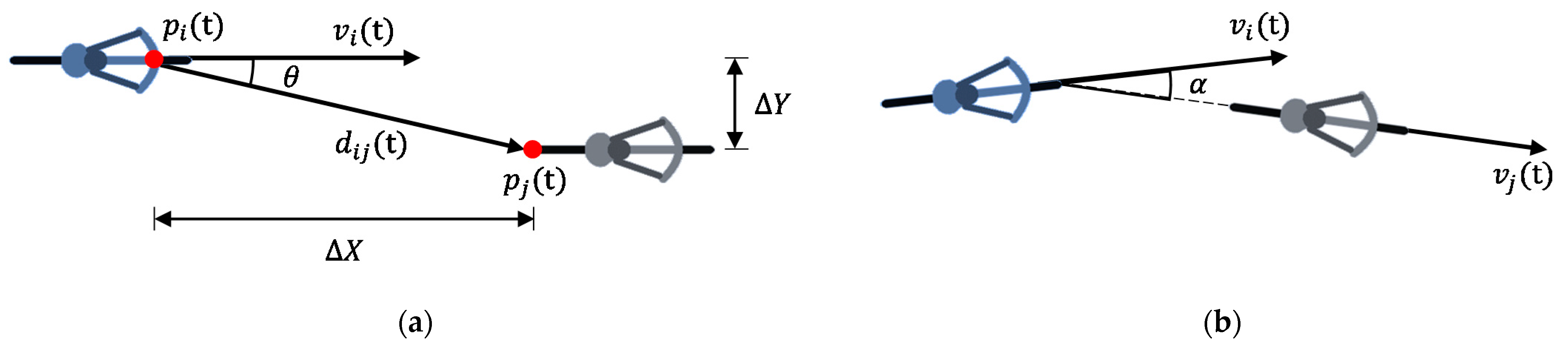
In a first step, situations in which the study participant followed and/or passed a simulated bicyclist in the bicycle lane are identified. Because no information is available concerning the lane used by the simulator participant, leading road users must be identified based on the trajectory data only. To this aim, two cosine similarities are applied. The first is used to determine whether the simulated road user lies in the direction of travel of the study participant at time , such that:
where
The second cosine similarity measure is applied to determine whether the direction of travel of the simulated road user is similar to that of participant at time :
The vectors and angles used to derive following situations are shown in Figure 1a,b.
Using the two cosine similarities defined in Equation (1) and Equation (4) and the distance between the road users Equation (2), the following intervals for each road user pair are determined. The beginning of the following interval is defined to be the first moment in which and and . The endpoint of the following interval is defined to be when or . Multiple following intervals can exist for each pair .
At any time , it is possible that the study participant followed more than one simulated bicyclist. This complicates the analyses significantly in comparison to lane-based traffic because reactions are not limited to one leading bicyclist. For simplification, the leading simulated bicyclist with the smallest distance is designated as the leading bicyclist at time . Following and passing situations are selected in which the bicyclist is designated as the leader for more than 10 s consecutively. To be considered in further analyses, the must fall below 10 m during the designated following interval. Although this approach greatly limited the number of following situations included in the dataset, it ensured that all speed adaptations during the selected following and passing events were made as a reaction to the given simulated bicyclist .
4. Results
By using the previously discussed microscopic trajectory data resulting from bicycle simulator rides, we introduce definitions of following and passing behavior of cyclists, calibrate the following parameters, and finally validate the calibrated parameters.
4.1. Following/Passing Behavior
Examples of the three types of following/passing behavior observed in the simulator study are shown in Figure 2.
The figure shows the longitudinal distance between the leader and the follower and the difference in velocity , where:
A total of 163 events in which a study participant passed and/or followed another bicyclist with a total duration greater than 10 s and containing a minimum distance between the following and leading road user of less than 10 m were extracted from the data. In the majority of passing events (116 events, 71.2%), study participants adjusted their speed and lateral position to pass a slower-moving simulated bicyclist without entering a following situation (Figure 2, left).
In 42 events (36.3%), the participant approached and followed a leading road user and then proceeded to pass the road user in the same lane (Figure 2, center). In 11 cases (6.7%), the participant approached a leading bicyclist, followed the leader for some time, and then fell behind the leader, exiting the following event (Figure 2, right).
4.2. Calibration of Following Parameters
The trajectories from the following and passing events are aggregated to derive average values for the Wiedemann 99 car-following model parameters , , and . is an important parameter that has a large influence on capacity. This parameter describes the time headway that a road user maintains while following another road user in addition to the time buffer provided by the standstill distance. According to [19], it can be derived from Equation (7).
The headway time is estimated for each observed following/passing events by defining during the following phase (blue in Figure 2) and the speed of the simulator study participant at that point. was set at 0.8 m based on the findings of [6]. The resulting cumulative density function of is shown in Figure 3.
The parameter quantifies the difference between the largest observed longitudinal distance and smallest distance during following (blue in Figure 2). is calculated for each following event and averaged over all observations. Only events in which the participant entered a following phase were included in the calculation of .
It was not possible to extract accurate estimates for the parameter , which describes the time in seconds that elapses between the start of deceleration during the approach phase and the beginning of the following phase. In many cases, the high volume of bicycle traffic on the simulated track prevented the observation of complete approach phases. In other cases, bicyclists alternated between accelerating and decelerating during the approach phase such that a duration of steady deceleration could not be identified.
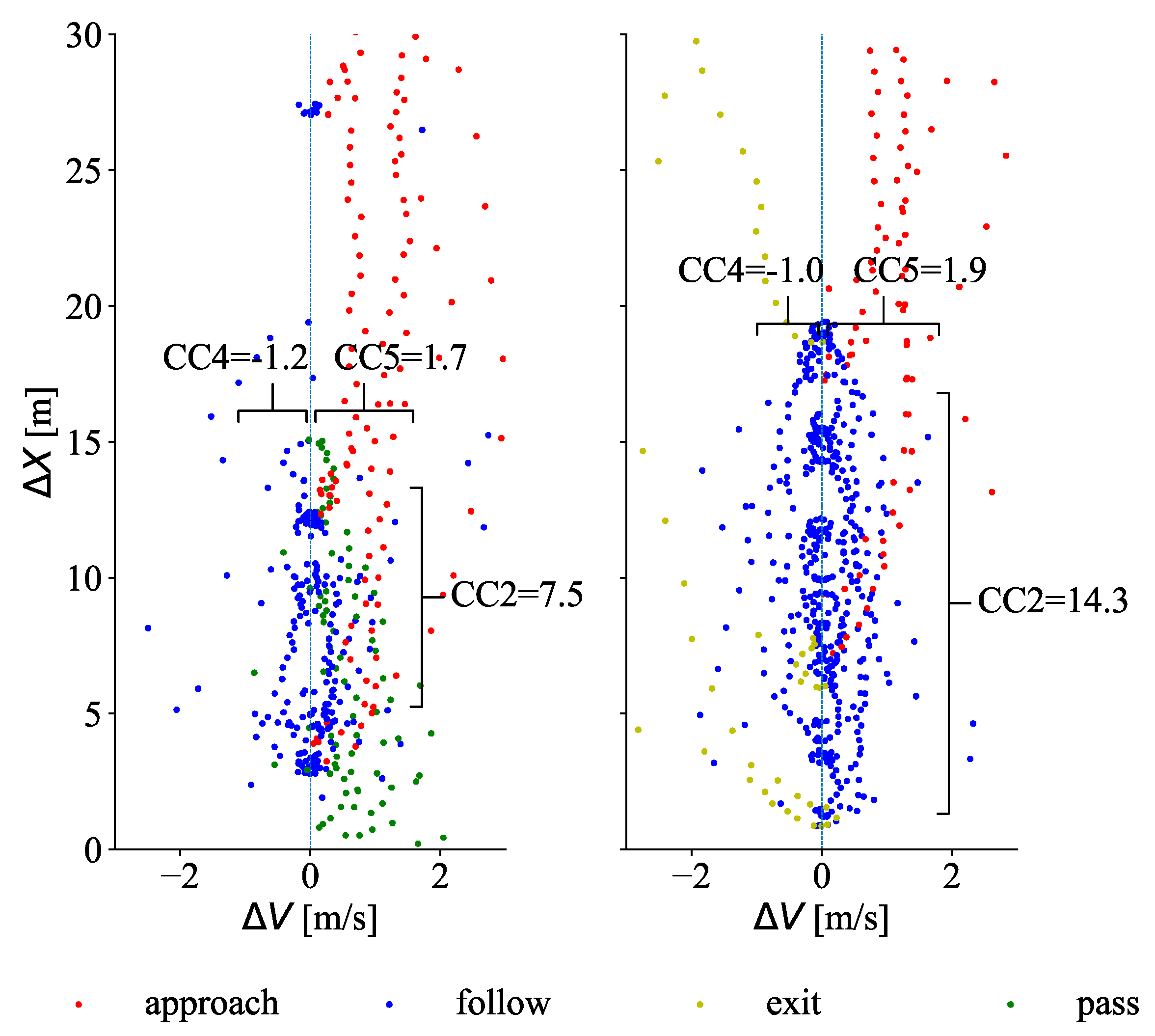
The parameters and describe the negative and positive relative velocity during the following phase. Here, and are found for each observed following phase. The results are averaged over all observations to estimate and , respectively. The resulting parameter estimates for , and are shown along with the observed data points in Figure 4.
The observation points and parameter estimates for following events that resulted in a pass are depicted on left. Data from events that were exited without a pass are shown on the right. Descriptive statistics of the parameter estimates are given in Table 2.
4.3. Validation
The calibrated parameters for the Wiedemann 99 car-following model and parameters controlling the lateral movement are listed in Table 3 (parameters highlighted in grey are the focus of the calibration presented in this paper). Two model parameter sets are tested: The first makes use of the car-following parameters suggested in the COWI report [11,13]. The second uses the parameter values from the analysis of the bicyclist simulator study trajectory data (observed, not simulated). In both cases, the parameters controlling the lateral behavior are calibrated by taking the suggested values from the COWI report and adjusting them to best represent the field conditions. The parameters controlling lateral behavior are the same for both of the tested parameter sets, which enables a direct comparison of the car-following model parameters.
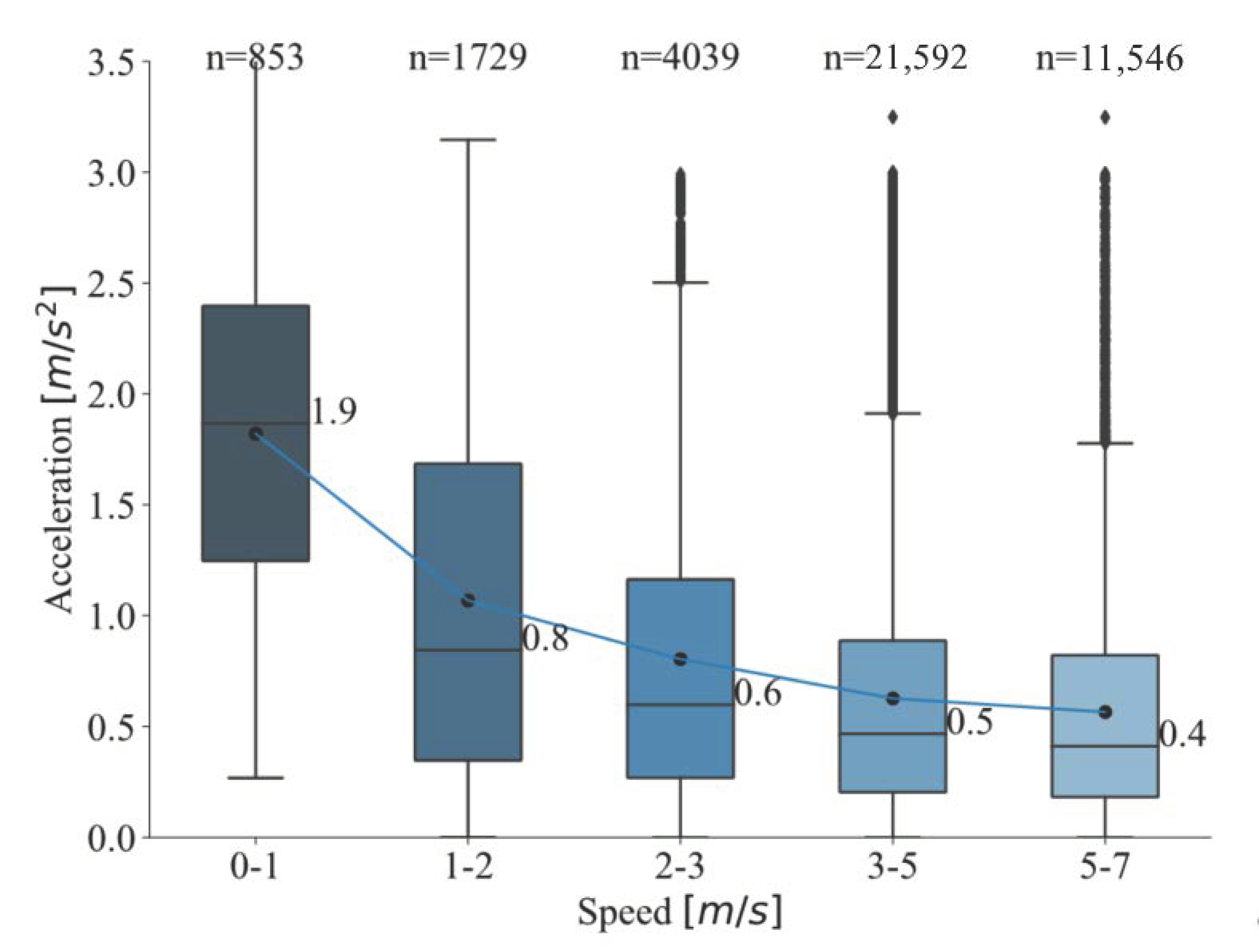
Other important parameters for the simulation are the desired acceleration function and desired speed distribution. Both of these parameters were calibrated based on the empirical studies carried out within the German research project “Traffic flow at signalized intersections with high bicycle traffic volumes” [12]. The desired acceleration function in Figure 5 was used for all simulated bicycle populations. The desired speed distribution for all bicyclists in the simulation was based on the findings of [12], where the 15th percentile , the 50th percentile , and the 85th percentile .
Three bicycle lanes are created in PTV Vissim with widths of 1.5 m, 1.8 m, and 2.5 m, reflecting the field conditions. Each simulation is run for one hour and is allowed 10 additional minutes for the network to fill before simulation data are collected. Ten runs are completed for each parameter set. The calibrated model parameter sets are validated using data collected within the German research project “Traffic flow at signalized intersections with high bicycle traffic volumes” [12]. The average queue dissipation time measured in seconds per bicyclist is used for validation [14].
where is the total queue dissipation time and is the number of bicyclists in the queue. The percent error and results of a t-test to determine significant differences in the means between the simulated and observed data are listed in Table 4. Bold text indicates that no significant difference between the means of the observed and simulated data was found.
Boxplots of the average queue dissipation time from the simulation runs and the field observations are shown in Figure 6. The horizontal bar in the boxplots represents the median and the white rectangle indicates the mean.
The capacities at the stop line delivered by the COWI report parameter set range between 1662 and 2268 bicyclists/h/m while those found using the trajectory data parameter set lie between 924 and 1250 bicyclists/h/m. Interestingly the highest capacities per meter width are found for the 1.8 m wide facility with both parameter sets.
5. Discussion
It is observed in the field that the average queue dissipation time decreases as the width of the bicycle lane increases as bicyclists can utilize the increased lateral space. The validation results for the 1.5 m wide bicycle lane are the most meaningful in assessing the car-following model parameters because the bicyclists move in a single file for a significant portion of the time in the simulation and in reality. As the width of the facility increases, the relevance of the lateral movement models correspondingly rises. The validation of both parameter sets showed a downward trend in the average queue dissipation time with increased facility width. However, the COWI report parameter set delivered results that were more constant across widths than the observations.
The trajectory data parameter set was able to very closely match the means of the observed dataset. However, both tested parameter sets failed to recreate the wide distribution that was observed in the field. The possibility to input a distribution of minimum lateral distances (standing and driving) for the simulated bicycle traffic rather than one value could potentially improve this problem. In general, the possibility to specify distributions for the following parameters would increase the variation to better match observed queue dissipation times.
The capacities found using the trajectory data parameter set are notably lower than those found using the COWI report parameter set. Capacity could not be extracted from the field data as the observed volume of bicycle traffic was not high enough. As estimates of bicycle facility range between 770 bicyclists/h/m and 4600 bicyclists/h/m [25], it is difficult to discern which capacity estimate is more correct.
The data used to calibrate the car-following model were collected in a bicycle simulator experiment, which raises well-founded questions about the realism of the results. Although a validation of the simulator indicated realistic speed and positioning, it is likely that the reaction to a real interacting bicyclist is somewhat different than the reaction to a simulated bicyclist in a virtual environment. Still, the approach for identifying and analyzing following events in non-lane based traffic, such as bicycle traffic, is valid and offers a starting point for other researchers. In addition, the simulated road environment is flat, eliminating the influence of inclinations that may be present in reality.
It is very difficult to obtain real data describing the interactions of road users over an extended period of time or space. Ossen and Hoogendoorn [10] used a helicopter to collect video data from a sufficiently long portion of a highway to analyze following behavior. Although this could be difficult in an urban context, other airborne instruments, such as drones, could be used for data collection [26].
The data used for this calibration were collected within the framework of a project examining bicycle highway design and signal control strategies for bicycle traffic (RASCH). Data describing a larger sample of complete following/passing events could be collected in a simulator study specifically designed for this purpose.
6. Conclusions
Microscopic trajectory data from a bicycle simulator study are used to estimate the following parameters of the Wiedemann 99 car-following model, which is implemented in the simulation software PTV Vissim. A method is suggested for identifying and isolating following/passing events from trajectory data without information describing the road geometry (e.g., location and width of bicycle lanes). An analysis of these following/passing events shows that bicyclists adapt their speed and lateral position to pass a leading bicycling without first entering a following phase in 71 % of passing events. The events in which a simulator study participant entered a following situation are analyzed to find the Wiedemann car-following parameters , , and . It was not possible to quantify the parameter due to the lack of consistent deceleration phases before entering the following phase. Validation of the parameter set identified from the trajectory data proved to provide a smaller percent error than the parameter set proposed by previous researchers.
The importance of the models controlling the lateral movement of simulated bicyclists and the calibration of these models cannot be overstated. Although this was not the focus of this paper, it is noted that these parameters arguably play a larger role in the realistic simulation of bicycle traffic than the following model parameters.
Future research will focus on other aspects of modelling cyclists in relation to varying different types and compositions of bicycles.
Author Contributions
Conceptualization, H.K., A.K. and K.B.; methodology, H.K.; software, H.K.; validation, H.K.; formal analysis, H.K., A.K. and K.B.; investigation, H.K., A.K. and K.B.; resources, H.K., A.K. and K.B.; data curation, H.K.; writing—original draft preparation, H.K., A.K. and K.B.; writing—review and editing, H.K., A.K. and K.B.; visualization, H.K.; supervision, H.K., A.K. and K.B.; project administration, H.K. and A.K.; funding acquisition, H.K. All authors have read and agreed to the published version of the manuscript.
Funding
The project RASCH is funded by the German Federal Ministry of Transport and Digital Infrastructure (BMVI) within the National Cycling Plan 2020 (NRVP).
Data Availability Statement
Data are available to interested parties from the authors upon request.
Acknowledgments
The trajectory data from the bicycle simulator were collected in the project RASCH (RAdSCHnellwege: Gestaltung effizienter und sicherer Infrastruktur). This project is funded by the German Federal Ministry of Transport and Digital Infrastructure within the National Cycling Plan 2020 (NRVP).
Conflicts of Interest
The authors declare no conflict of interest.
References
- Nobis, C. Mobilität in Deutschland—MiD: Analysen zum Radverkehr und Fußverkehr; BMVI: Bonn, Germany, 2019. [Google Scholar]
- Campisi, T.; Acampa, G.; Marino, G.; Tesoriere, G. Cycling master plans in Italy: The I-BIM feasibility tool for cost and safety assessments. Sustainability 2020, 12, 4723. [Google Scholar] [CrossRef]
- Nikiforiadis, A.; Basbas, S.; Campisi, T.; Tesoriere, G.; Garyfalou, M.I.; Meintanis, I.; Papas, T.; Trouva, M. Quantifying the Negative Impact of Interactions Between Users of Pedestrians-Cyclists Shared Use Space. In Proceedings of the International Conference on Computational Science and Its Applications, Cagliari, Italy, 1–4 July 2020; pp. 809–818. [Google Scholar]
- Campisi, T.; Deluka-Tibljaš, A.; Tesoriere, G.; Canale, A.; Rencelj, M.; Šurdonja, S. Cycling traffic at turbo roundabouts: Some considerations related to cyclist mobility and safety. Transp. Res. Procedia 2020, 45, 627–634. [Google Scholar] [CrossRef]
- Amprasi, V.; Politis, I.; Nikiforiadis, A.; Basbas, S. Comparing the microsimulated pedestrian level of service with the users’ perception: The case of Thessaloniki, Greece, coastal front. Transp. Res. Procedia 2020, 45, 572–579. [Google Scholar] [CrossRef]
- Grigoropoulos, G.; Keler, A.; Kaths, J.; Kaths, H.; Spangler, M.; Hoffmann, S.; Busch, F. Evaluation of the traffic efficiency of bicycle highways: A microscopic traffic simulation study. In Proceedings of the hEART2018, Toronto, ON, Canada, 20–22 June 2018. [Google Scholar]
- Grigoropoulos, G.; Hosseini, S.A.; Keler, A.; Kaths, H.; Spangler, M.; Busch, F.; Bogenberger, K. Traffic Simulation Analysis of Bicycle Highways in Urban Areas. Sustainability 2021, 13, 1016. [Google Scholar] [CrossRef]
- Twaddle, H.; Schendzielorz, T.; Fakler, O. Bicycles in urban areas: Review of existing methods for modeling behavior. Transp. Res. Rec. 2014, 2434, 140–146. [Google Scholar] [CrossRef]
- Fellendorf, M.; Vortisch, P. Validation of the microscopic traffic flow model VISSIM in different real-world situations. In Proceedings of the Transportation Research Board 80th Annual Meeting, Washington, DC, USA, 7–11 January 2001. [Google Scholar]
- Ossen, S.; Hoogendoorn, S.P. Car-following behavior analysis from microscopic trajectory data. Transp. Res. Rec. 2005, 1934, 13–21. [Google Scholar] [CrossRef]
- COWI. Micro Simulation of Cyclists in Peak Hour Traffic; COWI: Copenhagen, Denmark, 2013. [Google Scholar]
- Grigoropoulos, G.; Kaths, H.; Busch, F.; Baier, M.; Junghans, M.; Leonhardt, A. Verkehrsablauf an signalisierten Knotenpunkten mit hohem Radverkehrsaufkommen. In Proceedings of the HEUREKA 2020, Stuttgart, Germany, 1–2 April 2020. [Google Scholar]
- Aldred, R.; Best, L.; Jones, P. Cyclists in shared bus lanes: Could there be unrecognised impacts on bus journey times? In Proceedings of the Institution of Civil Engineers-Transport, London, UK, 12 July 2017; pp. 135–151. [Google Scholar]
- Carrignon, D. The Introduction of Bicycles and Motorcycles in a Large VISSIM Model Parliament Square; UCL: London, UK, 2009. [Google Scholar]
- Bahmankhah, B.; Coelho, M.C. Multi-objective optimization for short distance trips in an urban area: Choosing between motor vehicle or cycling mobility for a safe, smooth and less polluted route. Transp. Res. Procedia 2017, 27, 428–435. [Google Scholar] [CrossRef]
- Barceló, J. Fundamentals of Traffic Simulation; Springer: Berlin/Heidelberg, Germany, 2010; Volume 145. [Google Scholar]
- Kesting, A.; Treiber, M. Calibrating car-following models by using trajectory data: Methodological study. Transp. Res. Rec. 2008, 2088, 148–156. [Google Scholar] [CrossRef] [Green Version]
- Punzo, V.; Simonelli, F. Analysis and comparison of microscopic traffic flow models with real traffic microscopic data. Transp. Res. Rec. 2005, 1934, 53–63. [Google Scholar] [CrossRef]
- Durrani, U.; Lee, C.; Maoh, H. Calibrating the Wiedemann’s vehicle-following model using mixed vehicle-pair interactions. Transp. Res. Part C Emerg. Technol. 2016, 67, 227–242. [Google Scholar] [CrossRef]
- Hoogendoorn, S.; Hoogendoorn, R. Calibration of microscopic traffic-flow models using multiple data sources. Philos. Trans. R. Soc. A Math. Phys. Eng. Sci. 2010, 368, 4497–4517. [Google Scholar] [CrossRef] [PubMed]
- Busch, F.; Kaths, H.; Keler, A.; Hosseini, S.; Grigoropoulos, G.; Kaths, J. Fahrradsimulator: Anwendungsorientierter Erfahrungsbericht zu Aufbau und Nutzung; Lehrstuhl für Verkehrstechnik: Munich, Germany, 2019. [Google Scholar]
- Keler, A.; Kaths, J.; Chucholowski, F.; Chucholowski, M.; Grigoropoulos, G.; Spangler, M.; Kaths, H.; Busch, F. A bicycle simulator for experiencing microscopic traffic flow simulation in urban environments. In Proceedings of the 2018 21st International Conference on Intelligent Transportation Systems (ITSC), Maui, HI, USA, 4–7 November 2018; pp. 3020–3023. [Google Scholar]
- Azeem, A. Calibration and Validation of a Bicycle Simulator Using Real Bicycle Trajectories. Master’s Thesis, Technical University of Munich, Munich, Germany, 2019. [Google Scholar]
- Keler, A.; Kaths, H.; Grigoropoulos, G.; Hosseini, S.A.; Spangler, M.; Busch, F. RASCH-RAdSCHnellwege: Gestaltung effizienter und sicherer Infrastruktur. In Proceedings of the Nationaler Radverkehrskongress, Dresden, Germany, 13–14 May 2019. [Google Scholar]
- Hoogendoorn, S.; Daamen, W. Bicycle headway modeling and its applications. Transp. Res. Rec. 2016, 2587, 34–40. [Google Scholar] [CrossRef] [Green Version]
- Barmpounakis, E.; Geroliminis, N. On the new era of urban traffic monitoring with massive drone data: The pNEUMA large-scale field experiment. Transp. Res. Part C Emerg. Technol. 2020, 111, 50–71. [Google Scholar] [CrossRef]
Figure 1.
Vectors to identify following situations. (a) First cosine similarity measure. (b) Second cosine similarity measure.
Figure 1.
Vectors to identify following situations. (a) First cosine similarity measure. (b) Second cosine similarity measure.

Figure 2.
Examples of observed passing and following situations.

Figure 3.
Distribution for the headway time parameter .

Figure 4.
Observed points for following/passing events (left) and following/exiting events (right).

Figure 5.
Applied desired acceleration function.

Figure 6.
Observed and simulated average queue dissipation time.


Table 1.
Parameter values from the COWI report.
| Parameter | Values |
|---|---|
| CC0: Standstill distance | 0.20 m |
| CC1: Headway time | 0.5 s |
| CC2: Following variation | 2.00 m |
| CC3: Threshold for entering following | −20.00 |
| CC4: Negative following threshold | −0.25 |
| CC5: Positive following threshold | 0.25 |
| CC6: Speed dependency of oscillation | 1.00 |
| CC7: Oscillation acceleration | 0.20 m/s2 |
| CC8: Standstill acceleration | 1.80 m/s2 |
| CC9: Acceleration with 80 km/h | 0.01 m/s2 |
Table 2.
Descriptive statistics of the parameter estimates.
| Parameter | Passing Events | Exiting Events | ||
|---|---|---|---|---|
| s | s | |||
| CC2 [m] | 7.46 | 5.32 | 14.31 | 4.77 |
| CC4 [m/s] | −1.16 | 0.88 | −1.05 | 0.60 |
| CC5 [m/s] | 1.65 | 1.47 | 1.89 | 1.08 |
Table 3.
Parameters sets.
| Car-Following Parameters | COWI Report | Trajectory Data | |
|---|---|---|---|
| CC0 | 0.20 m | 0.80 | |
| CC1 | 0.5 s | Figure 3 | |
| CC2 | 2.00 m | 7.46 m | |
| CC3 | −20.00 | −20.00 | |
| CC4 | −0.25 | −1.16 | |
| CC5 | 0.25 | 1.65 | |
| CC6 | 1.00 | 0.00 | |
| CC7 | 0.20 m/s2 | 0.20 m/s2 | |
| CC8 | 1.80 m/s2 | 1.80 m/s2 | |
| CC9 | 0.01 m/s2 | 0.00 m/s2 | |
| Lateral Behavior Parameters | |||
| Desired position at free flow | any | ||
| Observe adjacent lane(s) | unselected | ||
| Diamond queuing | selected | ||
| Consider next turn | unselected | ||
| Collision time gain | 2.0 s | ||
| Minimum longitudinal speed | 3.6 km/h | ||
| Time between direction changes | 1.0 s | ||
| Overtake left | selected | ||
| Overtake right | selected | ||
| Minimum lateral distance standing | 0.20 m | ||
Table 4.
Evaluation of parameter sets based on .
| Width [m] | Parameter Set | % Error | T-Statistic | p-Value |
|---|---|---|---|---|
| 1.5 | COWI report | 43.0 | 7.217 | 0.000 |
| Trajectory data | 0.4 | −0.065 | 0.948 | |
| 1.8 | COWI report | 50.5 | 9.261 | 0.000 |
| Trajectory data | 10.4 | 1.810 | 0.072 | |
| 2.5 | COWI report | 41.3 | 5.818 | 0.000 |
| Trajectory data | 5.3 | −0.743 | 0.460 |
Publisher’s Note: MDPI stays neutral with regard to jurisdictional claims in published maps and institutional affiliations. |
© 2021 by the authors. Licensee MDPI, Basel, Switzerland. This article is an open access article distributed under the terms and conditions of the Creative Commons Attribution (CC BY) license (http://creativecommons.org/licenses/by/4.0/).
Share and Cite
MDPI and ACS Style
Kaths, H.; Keler, A.; Bogenberger, K. Calibrating the Wiedemann 99 Car-Following Model for Bicycle Traffic. Sustainability 2021, 13, 3487. https://0-doi-org.brum.beds.ac.uk/10.3390/su13063487
AMA Style
Kaths H, Keler A, Bogenberger K. Calibrating the Wiedemann 99 Car-Following Model for Bicycle Traffic. Sustainability. 2021; 13(6):3487. https://0-doi-org.brum.beds.ac.uk/10.3390/su13063487
Chicago/Turabian StyleKaths, Heather, Andreas Keler, and Klaus Bogenberger. 2021. "Calibrating the Wiedemann 99 Car-Following Model for Bicycle Traffic" Sustainability 13, no. 6: 3487. https://0-doi-org.brum.beds.ac.uk/10.3390/su13063487
Note that from the first issue of 2016, this journal uses article numbers instead of page numbers. See further details here.