A Multilevel Simulation Method for Time-Variant Reliability Analysis

Abstract

Crude Monte Carlo simulation (MCS) is the most robust and easily implemented method for performing time-variant reliability analysis (TRA). However, it is inefficient, especially for high reliability problems. This paper aims to present a random simulation method called the multilevel Monte Carlo (MLMC) method for TRA to enhance the computational efficiency of crude MCS while maintaining its accuracy and robustness. The proposed method first discretizes the time interval of interest using a geometric sequence of different timesteps. The cumulative probability of failure associated with the finest level can then be estimated by computing corrections using all levels. To assess the cumulative probability of failure in a way that minimizes the overall computational complexity, the number of random samples at each level is optimized. Moreover, the correction associated with each level is independently computed using crude MCS. Thereby, the proposed method can achieve the accuracy associated with the finest level at a much lower computational cost than that of crude MCS, and retains the robustness of crude MCS with respect to nonlinearity and dimensions. The effectiveness of the proposed method is validated by numerical examples.

1. Introduction

Reliability is an important measure of structures and systems [1,2,3,4]. It is defined as the probability that a structure or system successfully performs its intended function under specified conditions in a given time interval. Because of material degradation, time-variant loads, etc., a mechanical structure commonly has a time-variant response in performance function and its reliability decreases over service time. Accurately estimating reliability in the time interval of interest is extremely important for design optimization, reliability-based maintenance and risk control, which makes time-variant reliability analysis (TRA) methods urgently required in engineering. In recent decades, a number of methods have been developed for assessing time-variant reliability [5]. They can be generally divided into two categories, i.e., analytical methods [6,7,8,9] and sampling-based methods [10,11,12].

The representatives of analytical methods include first-crossing based methods [6,13] and time discretization-based methods [14,15]. After proposing the Rice formula, first-crossing based methods have gained much attention. Renaud et al. [7] presented an approach called PHI2, computing the outcrossing rate by solving a two-component parallel system reliability problem. Sudret [13] provided an analytical expression of the outcrossing rate in order to improve PHI2 in terms of accuracy. Despite the fact that classical first-crossing based methods are popular for TRA, they still experience poor accuracy because of the assumption that out-crossing events are mutually independent. Hu and Du [6] relaxed the assumption using the concept of joint crossing rate, and Yu et al. [16] proposed an approximation of the first-crossing probability density function (PDF) method to avoid directly computing the out-crossing rate. Meanwhile, time discretization-based methods were proposed in recent years, which implicitly accounted for the co-dependence among out-crossing events. Jiang et al. [14,17] transformed the time-variant reliability problem into a time-invariant series system reliability problem by employing stochastic process discretization and solving the transformed problem. Gong et al. [15] first discretized the time interval of interest into uniform time instants and then adopted the first order reliability method (FORM) to estimate instantaneous reliability at each instant. The time-variant reliability was finally computed by multivariate normal distribution function. Considering that the accuracy of time discretization-based methods relied on the discretization density (i.e., the number of time instants the considered time interval was discretized into), Zhang et al. [18] first approximated the trajectory of the most probable point of failure using a Kriging model and then transformed the stochastic process of the time-variant performance of a structure into an equivalent Gaussian process. Moreover, methods based on failure process decomposition [19], perturbation method [20], composite limit state [21] and total probability theorem [22] have also been proposed in the literature.

Compared with analytical methods, sampling-based methods present an advantage in robustness, especially for time-variant reliability problems with time-consuming models [23,24], e.g., finite element methods. The representatives of sampling-based methods include crude Monte Carlo simulation (MCS) [18], importance sampling (IS) [12,25,26], and subset simulation (SS) [27]. Yang et al. [25] proposed a method of deteriorating structures for TRA. The method was an extension of the cross-entropy-based adaptive importance sampling method for time-invariant reliability analysis [28] and was capable of dealing with multiple important regions. SS methods with Markov Chain Monte Carlo, or splitting methods, or both have shown their efficiency. Ching et al. [29] proposed SS with splitting to estimate the reliability of a dynamic system subject to stochastic excitation. The method employed splitting of a trajectory that reaches an intermediate failure level into multiple trajectories. Wang et al. [30] partitioned the stochastic process of time-variant performance into a series of correlated processes and adopted SS with splitting to reduce the computational cost. Du et al. [11] introduced the idea of parallel SS into TRA, and proposed a method to determine the so-called “principal variable” involved in parallel SS. Wang et al. [31] combined SS with splitting and time-variant copula function to estimate the cumulative probability of failure over a given time interval. To address time-variant problems involving a time-consuming performance function, Kriging [32,33] and polynomial chaos expansion [34,35] are commonly used in order to reduce the number of calls to time-consuming models. A limited number of samples are first used to train a surrogate model of the original performance function. Next, the cumulative probability of failure is estimated by a random sampling method. The strategies of determining the set of training samples are of the utmost importance for the accuracy and efficiency of surrogate model-based methods, on which a number of studies can be found [36,37]. For example, Jiang et al. [38] proposed an active failure-pursuing Kriging method to identify the most valuable samples for improving the accuracy of the Kriging model; Wang et al. [37] developed two methods based on projection outline adaptive Kriging to handle time-variant problems with random and interval uncertainties.

Even though a number of methods have been developed for TRA, crude MCS still has widespread use as reference and combined with other methods to enhance computational efficiency because of its robustness and easy implementation. However, its poor efficiency especially when dealing with high reliability problems impedes its extensive application in engineering. The widely used procedure of crude MCS can be summarized as: (1) discretizing the time interval of interest into uniform time instants and using the discretized instants to represent the continuous time interval; (2) generating random trajectories of the time-variant performance function and using performance values at discretized instants to determine whether a trajectory is safe or not. Subsequently, the cumulative probability of failure can be estimated. Note that the accuracy and efficiency of crude MCS rely on the number of discretized instants (or the associated timestep). Decreasing the discretized timestep means increasing its accuracy level, but reducing the efficiency. In order to enhance the computational efficiency of the procedure above, while retaining its accuracy, we present a sampling method called the multilevel Monte Carlo (MLMC) method. The idea of multilevel Monte Carlo path simulation is introduced into TRA. The so called Multilevel Monte Carlo path simulation was first developed by Giles for stochastic differential equations [39]. The method uses a geometric sequence of timesteps to discretize the considered time interval. The discretization error would be small, but the computational cost large if only the finest level were used. The situation would be reversed if only the coarsest level were used. To reduce the computational cost of computing the expectation of a random quantity defined by a stochastic differential equation, Giles [39] solved the problem on the finest level by estimating corrections using all the levels, thereby achieving the accuracy associated with the finest level at a lower cost. The idea is adopted herein, retaining the accuracy associated with the finest level but performing MCS at coarser levels to reduce the variance of the estimate of cumulative failure probability. The total number of function evaluations is minimized by optimizing the number of random trajectories allocated to each level.

The rest of the paper is organized as follows. Section 2 introduces the crude MCS for time-variant reliability analysis, including its main procedure in Section 2.1 and computational complexity in Section 2.2. MLMC for time-variant reliability analysis is elaborated in Section 3 and validated in Section 4. Section 5 provides the conclusions.

2. Crude MCS for Time-Variant Reliability Analysis

2.1. Crude MCS

This paper considers the time-variant performance function with the typical expression G(X,Z(t),t), where X is the vector of time-invariant random variables and Z(t) is the vector of stochastic processes. This special case G(X,Z(t),t) appears in many engineering scenarios, e.g., structures under stochastic loads and material degradation. We assume that G(X,Z(t),t) is computationally cheap and a function evaluation can be performed at any time τ. For problems with implicit and time-consuming performance function, one can build an asymptotically explicit expression through employing a surrogate model, such as Kriging and polynomial chaos expansion [34,38].

Without loss of generality, the failure of a structure, whose performance function is fully described by G(X,Z(t),t), is defined as G(X,Z(t),t) ≤ 0. In the time interval of interest [0, T], a failure event occurs if the response value of the performance function G(X,Z(t),t) crosses the failure threshold 0. Accordingly, the cumulative probability of failure can be expressed as,

$$\begin{array}{cc}{P}_{\mathrm{f},\mathrm{c}}(0,T)& =\mathrm{Pr}\left\{\exists \tau \in [0,T]|G(\mathit{X},\mathit{Z}(\tau ),\tau )\le 0\right\}\hfill \\ & =\mathrm{Pr}\left\{\underset{0\le \tau \le T}{\min }\{G(\mathit{X},\mathit{Z}(\tau ),\tau )\}\le 0\right\}\hfill \end{array}$$

(1)

where $\mathrm{Pr}\{\cdot \}$ is the probability operator, and “$\exists$” means “there exists”. Herein, the failure indicator function I(x,z(t)) is introduced, whose expression is,

$$I\left(\mathit{x},\mathit{z}(t)\right)=\{\begin{array}{l}1 \underset{0\le \tau \le T}{\min }\{G(\mathit{x},\mathit{z}(\tau ),\tau )\}\le 0\\ 0 \mathrm{otherwise}\end{array}$$

(2)

where z(t) is a trajectory of Z(t). Thus, P_f,c(0,T) can be rewritten as follows:

$$P_{\mathrm{f},\mathrm{c}}(0,T)=\mathrm{Pr}\left\{I\left(\mathit{X},\mathit{Z}(\tau )\right)=1\right\}=E\left\{I\left(\mathit{X},\mathit{Z}(\tau )\right)\right\}$$

(3)

As illustrated in Section 1, crude MCS is the most robust method to estimate P_f,c(0, T). It is commonly implemented as follows:

Step 1: Discretize the time interval [0, T] into K + 1 uniform instants with time step Δt. For convenience of the illustration below, we control the number of discretized time instants and the corresponding timestep using two positive integers, i.e., K₀ and L.

$$K=K_0\cdot 2^L\mathrm{and}\Delta t=T/K$$

(4)

Then, P_f,c(0,T) can be approximated by:

$$P_{\mathrm{f},\mathrm{c}}(0,T)=\underset{K\to \infty }{\lim }E\left\{I^{(L)}\left(\mathit{X},\mathit{Z}(\tau )\right)\right\}\approx E\left\{I^{(L)}\left(\mathit{X},\mathit{Z}(\tau )\right)\right\}$$

(5)

Let $P_{\mathrm{f},\mathrm{c}}^{(L)}(0,T)$ denote the approximation of the cumulative probability of failure:

$$P_{\mathrm{f},\mathrm{c}}^{(L)}(0,T)=E\left\{I^{(L)}\left(\mathit{X},\mathit{Z}(\tau )\right)\right\}$$

(6)

where I^(L)(x,z(t)) is an approximation of the indicator function I(x,z(t)):

$$I^{(L)}\left(\mathit{x},\mathit{z}(t)\right)=\{\begin{array}{l}1 \underset{0\le k\le K}{\min }\{G(\mathit{x},\mathit{z}({\tau }_k),{\tau }_k)\}\le 0\\ 0 \mathrm{otherwise}\end{array}$$

(7)

Step 2: Generate i.i.d. (independent and identically distributed) samples of X and trajectories of Z(t), and estimate P_f,c(0,T) according to the law of large numbers:

$$P_{\mathrm{f},\mathrm{c}}(0,T)\approx P_{\mathrm{f},\mathrm{c}}^{(L)}(0,T)\approx \frac{1}{N_{\mathrm{MC}}}{\displaystyle \sum _{n=1}^{N_{\mathrm{MC}}}{I}^{(L)}\left({\mathit{x}}_n,{\mathit{z}}_n(t)\right)}$$

(8)

where N_MC is the number of random simulations crude MCS performs. Multiple techniques are capable of generating random trajectories of stochastic processes, e.g., the expansion optimal linear estimation method (EOLE) and Karhunen-Loève (KL) expansion are widely used in the literature [40,41,42]. In the section of method validation below, EOLE is adopted.

Let ${\widehat{P}}_{\mathrm{f},\mathrm{c}}^{\mathrm{MC}}(0,T)$ denote the estimate obtained by crude MCS:

$${\widehat{P}}_{\mathrm{f},\mathrm{c}}^{\mathrm{MC}}(0,T)=\frac{1}{N_{\mathrm{MC}}}{\displaystyle \sum _{n=1}^{N_{\mathrm{MC}}}{I}^{(L)}\left({\mathit{x}}_n,{\mathit{z}}_n(\tau )\right)}$$

(9)

It is worth noting that the error in the estimate ${\widehat{P}}_{\mathrm{f},\mathrm{c}}^{\mathrm{MC}}(0,T)$ can be asymptotically determined using the following equation:

$$|{\widehat{P}}_{\mathrm{f},\mathrm{c}}^{\mathrm{MC}}(0,T)-P_{\mathrm{f},\mathrm{c}}(0,T)|\approx \left|E\left\{I^{(L)}\left(\mathit{X},\mathit{Z}(\tau )\right)\right\}-P_{\mathrm{f},\mathrm{c}}(0,T)\right|+\left|{\widehat{P}}_{\mathrm{f},\mathrm{c}}^{\mathrm{MC}}(0,T)-E\left\{I^{(L)}\left(\mathit{X},\mathit{Z}(\tau )\right)\right\}\right|$$

(10)

The first term is the bias introduced by the uniform discretization, and the second term corresponds to the error due to the random sampling. Given values of N₀ and L, this paper uses a multilevel method to reduce the error caused by MCS, leaving unchanged the bias due to the discretization.

The coefficient of variation associated with ${\widehat{P}}_{\mathrm{f},\mathrm{c}}^{\mathrm{MC}}(0,T)$ is:

$${\mathrm{cov}}_{P\mathrm{f}}=\frac{\sqrt{\mathrm{var}\left({\widehat{P}}_{\mathrm{f},\mathrm{c}}^{\mathrm{MC}}(0,T)\right)}}{P_{\mathrm{f},\mathrm{c}}^{(L)}(0,T)}$$

(11)

where

$$\mathrm{var}\left({\widehat{P}}_{\mathrm{f},\mathrm{c}}^{\mathrm{MC}}(0,T)\right)=\frac{P_{\mathrm{f},\mathrm{c}}^{(L)}(0,T)\left(1-P_{\mathrm{f},\mathrm{c}}^{(L)}(0,T)\right)}{N_{\mathrm{MC}}}$$

(12)

2.2. Computational Cost of Crude MCS

Given a realization of X and a trajectory of Z(t) (e.g., x_n and z_n(t)), $K_0\cdot 2^L+1$ evaluations of the time-variant performance function G(X,Z(t),t) are needed in order to determine the value of $I^{(L)}\left({\mathit{x}}_n,{\mathit{z}}_n(\tau )\right)$. This paper ignores the asymptotically negligible cost of generating random realizations of X and trajectories of Z(t), and uses the number of function evaluations to measure the computational cost of crude MCS as well as the method proposed in Section 3.

According to Equations (11) and (12), to achieve a coefficient of variation smaller than δ_Pf, i.e.,

$${\mathrm{cov}}_{P\mathrm{f}}<{\delta }_{P\mathrm{f}}$$

(13)

the number of trajectories of G(X,Z(t),t), i.e., N_MC, needs to satisfy that:

$$N_{\mathrm{MC}}>\frac{1-P_{\mathrm{f},\mathrm{c}}^{(L)}(0,T)}{{\delta }_{P\mathrm{f}}^2{P}_{\mathrm{f},\mathrm{c}}^{(L)}(0,T)}$$

(14)

Hence, the computational cost of crude MCS corresponding to the accuracy requirement δ_Pf, i.e., the total number of function evaluations, is:

$$C_{\mathrm{S}}=\frac{1-P_{\mathrm{f},\mathrm{c}}^{(L)}(0,T)}{{\delta }_{P\mathrm{f}}^2{P}_{\mathrm{f},\mathrm{c}}^{(L)}(0,T)}(K_0\cdot 2^L+1)$$

(15)

3. Multilevel Monte Carlo for Time-Variant Reliability Analysis

Crude MCS is capable of achieving any required accuracy regardless of nonlinearity and dimensions of the time-variant performance function if K and N_MC are sufficiently large. However, its commonly computationally expensive. To overcome this issue, multilevel Monte Carlo is applied herein to deal with TRA.

MLMC discretizes the time interval [0, T] using a geometric sequence of different timesteps $\Delta t_l=T/(K_0\cdot 2^l)$ (l = 0,…,L). The smallest timestep $\Delta t_L$ corresponds to the discretization bias defined by the first term of Equation (10). The multilevel method optimizes the computational cost on each level in order to reduce the overall computational complexity of estimating the cumulative probability of failure, retaining the accuracy associated with the level L.

3.1. Multilevel Monte Carlo

Consider a sequence of approximations $\left\{P_{\mathrm{f},\mathrm{c}}^{(l)}(0,T)\right\}$ of the cumulative failure probability with different timesteps. It is clearly true that $P_{\mathrm{f},\mathrm{c}}^{(l)}(0,T)$ approximates to P_f,c(0,T) with an increasing accuracy as the increase of level l, but the computational complexity also increases with l. MLMC utilizes the characteristic of $P_{\mathrm{f},\mathrm{c}}^{(l)}(0,T)$ (l < L) to reduce the computational complexity of $P_{\mathrm{f},\mathrm{c}}^{(L)}(0,T)$. It first expresses $P_{\mathrm{f},\mathrm{c}}^{(L)}(0,T)$ in terms of a linear combination of $P_{\mathrm{f},\mathrm{c}}^{(l)}(0,T)$ (l = 0, …, L), and then optimizes the computational cost allocated to each level l.

$P_{\mathrm{f},\mathrm{c}}^{(L)}(0,T)$ can be rewritten as:

$$P_{\mathrm{f},\mathrm{c}}^{(L)}(0,T)=P_{\mathrm{f},\mathrm{c}}^{(0)}(0,T)+\left(P_{\mathrm{f},\mathrm{c}}^{(1)}(0,T)-P_{\mathrm{f},\mathrm{c}}^{(0)}(0,T)\right)+\dots +\left(P_{\mathrm{f},\mathrm{c}}^{(L)}(0,T)-P_{\mathrm{f},\mathrm{c}}^{(L-1)}(0,T)\right)$$

(16)

Then, it is easily concluded that:

$$P_{\mathrm{f},\mathrm{c}}^{(L)}(0,T)=P^{(0)}+P^{(1)}+\dots +P^{(L)}$$

(17)

where

$$\begin{gathered} P^{(0)}=E\left\{I^{(0)}\left(\mathit{X},\mathit{Z}(\tau )\right)\right\}\mathrm{and}{P}^{(l)}=E\left\{\Delta I^{(l)}\left(\mathit{X},\mathit{Z}(\tau )\right)\right\} \\ \Delta I^{(l)}\left(\mathit{X},\mathit{Z}(\tau )\right)=I^{(l)}\left(\mathit{X},\mathit{Z}(\tau )\right)-I^{(l-1)}\left(\mathit{X},\mathit{Z}(\tau )\right) \\ l=1,2,\text{…},L \end{gathered}$$

(18)

MLMC independently estimates each expectation on the right side of Equation (17). An unbiased estimate of the cumulative probability of failure is then obtained, which has the following expression:

$${\widehat{P}}_{\mathrm{f},\mathrm{c}}^{\mathrm{ML}}(0,T)={\widehat{P}}^{(0)}+{\widehat{P}}^{(1)}+\dots +{\widehat{P}}^{(L)}$$

(19)

where

$$\begin{gathered} {\widehat{P}}^{(0)}=\frac{1}{N_0}{\displaystyle \sum _{n=1}^{N_0}{I}^{(0)}\left({\mathit{x}}_{0,n},{\mathit{z}}_{0,n}(\tau )\right)}\mathrm{and}{\widehat{P}}^{(l)}=\frac{1}{N_l}{\displaystyle \sum _{n=1}^{N_l}\Delta I^{(l)}\left({\mathit{x}}_{l,n},{\mathit{z}}_{l,n}(\tau )\right)} \\ l=1,2,\text{…},L \end{gathered}$$

(20)

N_l represents the number of random simulations on level l to estimate ${\widehat{P}}^{(l)}$ (l = 0,…,L). The coefficient of variation of the multilevel estimate ${\widehat{P}}_{\mathrm{f},\mathrm{c}}^{\mathrm{ML}}(0,T)$ can be calculated as:

$${\mathrm{cov}}_{P\mathrm{f}}=\frac{\sqrt{\mathrm{var}\left({\widehat{P}}_{\mathrm{f},\mathrm{c}}^{\mathrm{ML}}(0,T)\right)}}{P_{\mathrm{f},\mathrm{c}}^{(L)}(0,T)}$$

(21)

where $\mathrm{var}\left({\widehat{P}}_{\mathrm{f},\mathrm{c}}^{\mathrm{ML}}(0,T)\right)$ is the variance of ${\widehat{P}}_{\mathrm{f},\mathrm{c}}^{\mathrm{ML}}(0,T)$:

$$\mathrm{var}\left({\widehat{P}}_{\mathrm{f},\mathrm{c}}^{\mathrm{ML}}(0,T)\right)={\displaystyle \sum _{l=0}^L\frac{P^{(l)}\cdot (1-P^{(l)})}{N_l}}$$

(22)

According to Equations (7) and (18), determining the value of $\Delta I^{(l)}\left(x,z(\tau )\right)$ needs $K_0\cdot 2^l+1$ function evaluations. Therefore, the total number of function evaluations MLMC needs is,

$$C_{\mathrm{M}}={\displaystyle \sum _{l=0}^L{N}_l(K_0\cdot 2^l+1)}$$

(23)

In order to acquire an estimate ${\widehat{P}}_{\mathrm{f},\mathrm{c}}^{\mathrm{ML}}(0,T)$ whose coefficient variation satisfies Equation (13), the combination of [N₀,…,N_L] must meet with:

$${\displaystyle \sum _{l=0}^L\frac{P^{(l)}\cdot (1-P^{(l)})}{N_l}}<{\left({\delta }_{P\mathrm{f}}\cdot P_{\mathrm{f},\mathrm{c}}^{(L)}(0,T)\right)}^2$$

(24)

It is noticed that a great number of combinations of (N₀, …, N_L) are available but computational costs associated with the combinations may be considerably different. For given K₀ and L, the combination of (N₀, …, N_L) is optimal if it requires the least number of function evaluations while maintaining the coefficient variation of ${\widehat{P}}_{\mathrm{f},\mathrm{c}}^{\mathrm{ML}}(0,T)$ smaller than the prescribed threshold δ_Pf. That is to say, one can obtain the optimal (N₀, …, N_L) (i.e., $[N_0^{\ast },\dots ,N_L^{\ast }]$) by solving the optimization problem below:

$$\begin{array}{l}[N_0^{\ast },\dots ,N_L^{\ast }]=\arg \min {\displaystyle \sum _{l=0}^L{N}_l(K_0\cdot 2^l+1)}\\ \{\begin{array}{l}{\displaystyle \sum _{l=0}^L\frac{P^{(l)}\cdot (1-P^{(l)})}{N_l}}<{\left({\delta }_{P\mathrm{f}}\cdot P_{\mathrm{f},\mathrm{c}}^{(L)}(0,T)\right)}^2\\ N_l\ge 0 (l=0,\dots ,L)\end{array}\end{array}$$

(25)

Treating N_l (l = 0, …, L) as continuous variables, the optimal number of random simulations on level l is easily obtained using the Lagrange Multiplier method:

$$N_l^{\ast }=\frac{1}{{\left({\delta }_{P\mathrm{f}}\cdot P_{\mathrm{f},\mathrm{c}}^{(L)}(0,T)\right)}^2}\sqrt{\frac{V_l}{C_l}}\sum _{l=0}^L\sqrt{V_l\cdot C_l}$$

(26)

where

$$V_l=P^{(l)}\cdot (1-P^{(l)})\mathrm{and}{C}_l=K_0\cdot 2^l+1$$

(27)

We denote the computational cost associated with $[N_0^{\ast },\dots ,N_L^{\ast }]$ by $C_{\mathrm{M}}^{\ast }$. According to the optimal allocation of computational resource determined by Equation (26), one can implement the MLMC method and estimate the cumulative probability of failure in a way that minimizes the computational complexity.

3.2. Implementation of MLMC

Equation (26) indicates that the knowledge of V_l and $P_{\mathrm{f},\mathrm{c}}^{(L)}(0,T)$ is essential for calculating the optimal numbers of simulations MLMC needs to perform on each level l and judging whether or not MLMC is more efficient than crude MCS by comparing C_S (Equation (15)) with $C_{\mathrm{M}}^{\ast }$ (Equations (23) and (26)). However, values of V_l and $P_{\mathrm{f},\mathrm{c}}^{(L)}(0,T)$ are unavailable before performing TRA. Therefore, it is difficult to make a decision in practical engineering on employing MLMC or crude MCS to assess the time-variant reliability of a mechanical structure or system, and the optimal allocation of computational cost is hardly obtained in advance if MLMC is adopted.

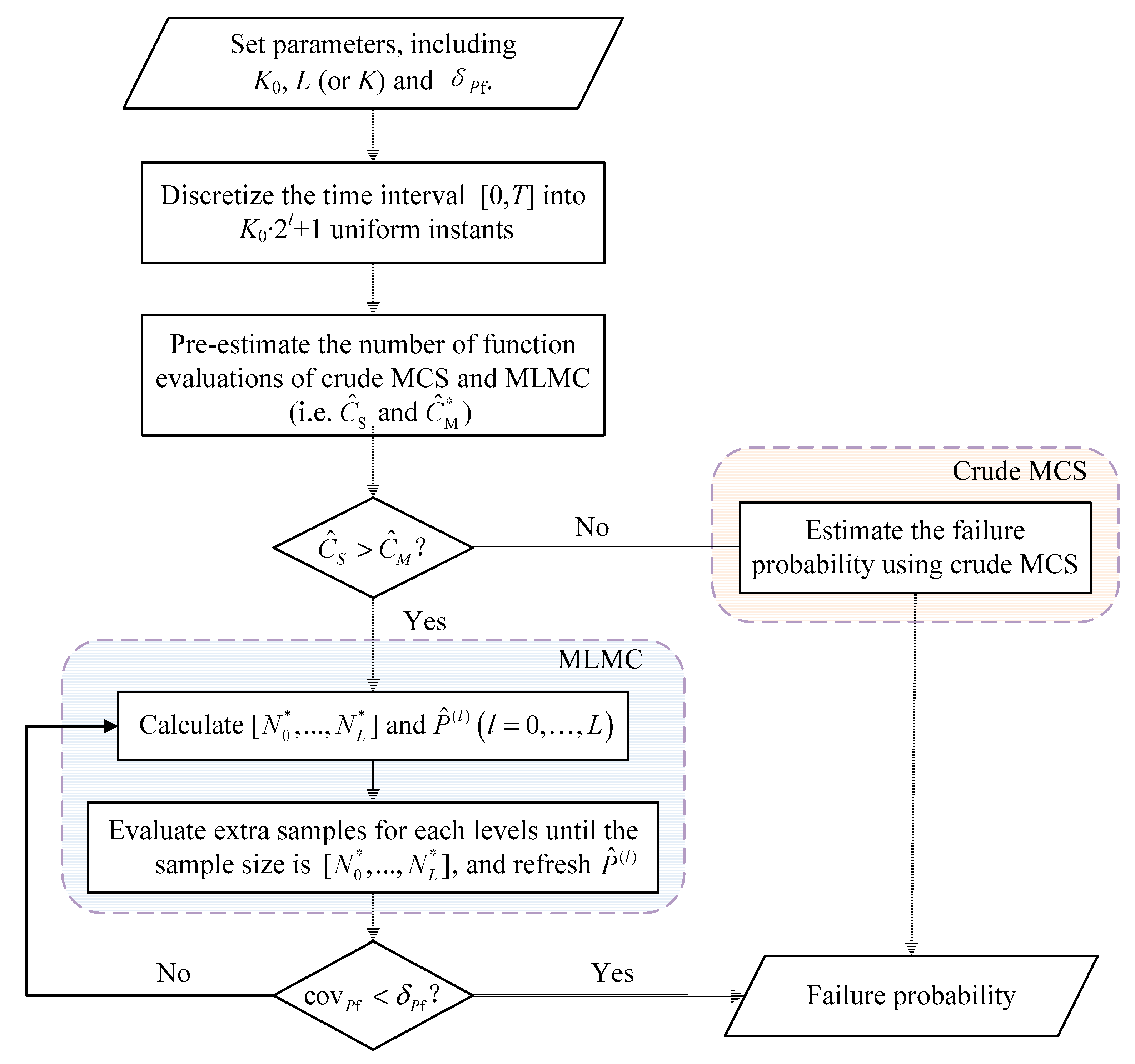
In order to address the issues above, this subsection proposes a procedure for TRA to adaptively choose the more efficient method between crude MCS and MLMC. The flowchart is given by Figure 1. It consists of eight steps:

Step 1 Set values of parameters, including K₀, L (or K) and δ_Pf.

This paper sets K₀ = 10. It will be verified in Section 4 that K₀ has little effect on the efficiency of MLMC. One can set L (or K) and δ_Pf according to the accuracy requirement of TRA. According to Equation (10), the accuracy of MLMC as well as crude MCS increases with L and decreases with the threshold of the coefficient of variation δ_Pf.

Step 2 Discretize the time interval of interest [0,T] into $K_0\cdot 2^l+1$ uniform instants (l = 0,…,L).

The relationship between the accuracy level of $P_{\mathrm{f},\mathrm{c}}^{(L)}(0,T)$ and the largest number of discretized time instants $K_0\cdot 2^L+1$ is still an open issue, which is not discussed in this paper.

Step 3 Pre-estimate the number of function evaluations of crude MCS and MLMC.

According to Equations (15), (23) and (26), P^(l) (l = 0, …, L) are essential for calculating C_S and $C_{\mathrm{M}}^{\ast }$. However, considerable samples are needed if one independently estimates each P^(l) (l = 0, …, L). In order to reduce the computational cost of the pre-estimate, this step makes an assumption that P⁽⁰⁾ ≈ P⁽¹⁾ ≈ … ≈ P^(L). Thus, only P⁽⁰⁾ is needed to pre-estimate the computational cost of crude MCS and MLMC.

Generate random sample set S₀:

$$S_0=\left\{\left({\mathit{x}}_{0,n},z_{0,n}(\tau )\right)|n=1,\dots ,N_0\right\}$$

(28)

Then, estimate P⁽⁰⁾ as follows:

$${\widehat{P}}^{(0)}=\frac{1}{N_0}{\displaystyle \sum _{n=1}^{N_0}{I}^{(0)}\left({\mathit{x}}_{0,n},{\mathit{z}}_{0,n}(\tau )\right)}$$

(29)

This step sets N₀ meeting with the following accuracy requirement:

$$\mathrm{cov}({\widehat{P}}^{(0)})\le 0.2$$

(30)

Under the assumption made above, the computational cost of crude MCS and MLMC can be pre-estimated according to Equations (15), (23) and (26).

Step 4 If ${\widehat{C}}_{\mathrm{S}}>{\widehat{C}}_{\mathrm{M}}^{\ast }$, MLMC is more efficient and adopted to estimate the cumulative probability of failure. Continue the procedure to Step 5. Otherwise, crude MCS is adopted and the procedure goes to Step 7.

Step 5 Implement MLMC as follow:

(a) Calculate $[N_0^{\ast },\dots ,N_L^{\ast }]$ according to Equation (26) and the current ${\widehat{P}}^{(l)}$ (l = 0, …, L). Considering that ${\widehat{P}}^{(l)}$ pre-estimated in Step 3 may have a large error, we provisionally set the accuracy requirement equal to 2δ_Pf in the first iteration and restore it to δ_Pf after the first iteration.

(b) Supplement S_l with random samples and increase the number of samples in S_l to $N_l^{\ast }$ (l = 0, …, L).

(c) Refresh ${\widehat{P}}^{(l)}$ according to Equation (20).

Step 6 Calculate ${\widehat{P}}_{\mathrm{f},\mathrm{c}}^{\mathrm{ML}}(0,T)$ and the corresponding ${\mathrm{cov}}_{P\mathrm{f}}$ according to Equations (19) and (21), respectively. If ${\mathrm{cov}}_{P\mathrm{f}}<{\delta }_{P\mathrm{f}}$, ${\widehat{P}}_{\mathrm{f},\mathrm{c}}^{\mathrm{ML}}(0,T)$ is accurate enough, the procedure stops. The last estimate of the cumulative probability of failure is regarded as the result of the procedure; otherwise, go back to Step 5.

Step 7 Estimate the cumulative probability of failure using crude MCS according to Equations (9) and (14).

Step 8 Output the estimate of cumulative probability of failure.

4. Numerical Validation

This section aims to validate the computational efficiency of the method proposed in Section 3. In the validation, the proposed method is only compared with crude MCS in terms of the total number of function evaluations. As a large number of function evaluations is needed by both methods, examples studied in this section have explicit performance functions.

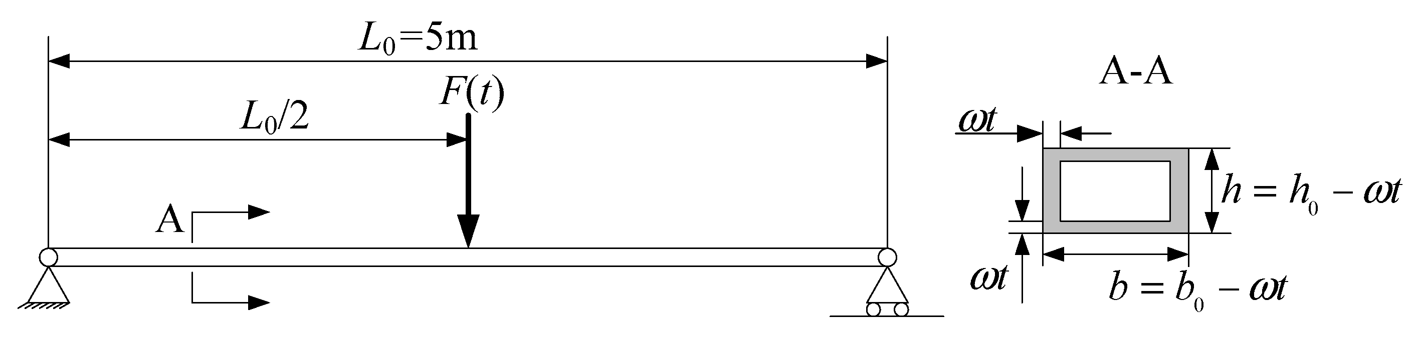
4.1. A Steel Bending Beam

As depicted by Figure 2, the first example studies a steel bending beam whose cross section evolves linearly in time because of isotropic corrosion. The beam is submitted to two loads, i.e., a dead load p = ρ_stb₀h₀ caused by the gravity and a pinpoint load F(t) modeled by a Gaussian process. The time-variant performance function of the beam is given by:

$$G(\mathit{X},F(t),t)=\frac{b(t)h^2(t)}{4}-\left(\frac{F(t)L_0}{4}+\frac{{\rho }_{st}{b}_0{h}_0{L}^2}{8}\right)$$

(31)

where X = [f_y,b₀,h₀]^T. The time interval of interest is (0, 20 year).

Table 1. The input parameters (example 1).

Variable	Distribution	Mean	Standard Deviation	Autocorrelation Coefficient Function
fy	Lognormal	240 MPa	24 MPa	-
b0	Lognormal	0.2 m	0.01 m	-
h0	Lognormal	0.04 m	0.004 m	-
F(t)	Gaussian	3500 N	700 N	exp(−(t2 − t1)2)
ρst	Deterministic	78.5 kN/m3	-	-
ω	Deterministic	0.03 mm/year	-	-

gathers the input parameters of the time-variant performance function.

This subsection regards crude MCS with 10⁹ random simulations as the reference to compute P^(l) and $P_{\mathrm{f},\mathrm{c}}^{(l)}(0,T)$ (K₀ = 5 and L = 8), as shown by Figure 3. It can be found that P^(l) decreases dramatically with the increase of l. To investigate the performance of the proposed method, it is implemented with several combinations of (K, δ_Pf, K₀). Results coming from the proposed MLMC and crude MCS are summarized in

Table 2. Results of the steel bending beam. N_call denotes the total number of calls to the time-variant performance function, and δ represents the coefficient of variation associated with ${\widehat{P}}_{\mathrm{f},\mathrm{c}}$.

K	δPf	K0	Method	${\widehat{\mathit{P}}}_{\mathbf{f},\mathbf{c}}$	Ncall	δ
640	-	-	Benchmark	1.24 × 10−4	-	2.8 × 10−3
	0.03	-	Crude Monte Carlo simulation (MCS)	1.19 × 10−4	6.01 × 109	3.0 × 10−2
		5	The proposed method	1.27 × 10−4	2.22 × 109	2.96 × 10−2
		10		1.21 × 10−4	1.86 × 109	2.92 × 10−2
		20		1.28 × 10−4	2.04 × 109	2.86 × 10−2
		40		1.23 × 10−4	1.71 × 109	2.87 × 10−2
		80		1.23 × 10−4	2.05 × 109	2.89 × 10−2
640	0.1	10	Crude MCS	1.14 × 10−4	5.7 × 108	9.95 × 10−3
			The proposed method	1.25 × 10−4	1.68 × 108	9.04 × 10−2
	0.05		Crude MCS	1.17 × 10−4	2.19 × 109	4.99 × 10−2
			The proposed method	1.18 × 10−4	5.04 × 108	4.99 × 10−2
	0.03		Crude MCS	1.19 × 10−4	6.01 × 109	3.0 × 10−2
			The proposed method	1.21 × 10−4	1.86 × 109	2.92 × 10−2
	0.01		Crude MCS	1.24 × 10−4	5.15 × 1010	1.0 × 10−3
			The proposed method	1.22 × 10−4	1.74 × 1010	9.7 × 10−3
320	0.03	10	Benchmark	1.23 × 10−4	-	2.8 × 10−3
			Crude MCS	1.25 × 10−4	2.85 × 109	3.0 × 10−2
			The proposed method	1.24 × 10−4	1.48×109	2.86 × 10−2
640			Benchmark	1.24 × 10−4	-	2.8 × 10−3
			Crude MCS	1.19 × 10−4	6.01 × 109	3.0 × 10−2
			The proposed method	1.21 × 10−4	1.86 × 109	2.92 × 10−2
1280			Benchmark	1.24 × 10−4	-	2.8 × 10−3
			Crude MCS	1.23 × 10−4	1.15 × 1010	3.0 × 10−2
			The proposed method	1.23 × 10−4	2.36 × 109	2.94 × 10−2

. According to the presented results, the proposed method remarkably reduces the total number of function evaluations while both methods achieve the level of accuracy satisfying the threshold of the coefficient of variation δ_Pf. It is worth mentioning that all results coming from the proposed procedure are achieved using MLMC. Integrating crude MCS into the proposed procedure is to account for special cases in which MLMC needs more computational cost even though we have not yet encountered such cases.

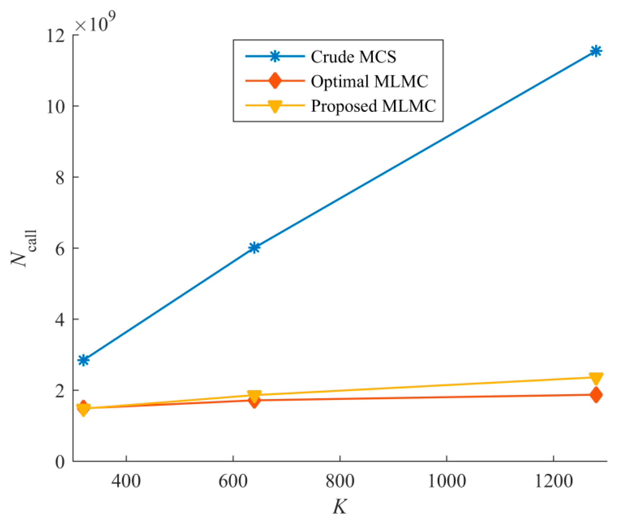
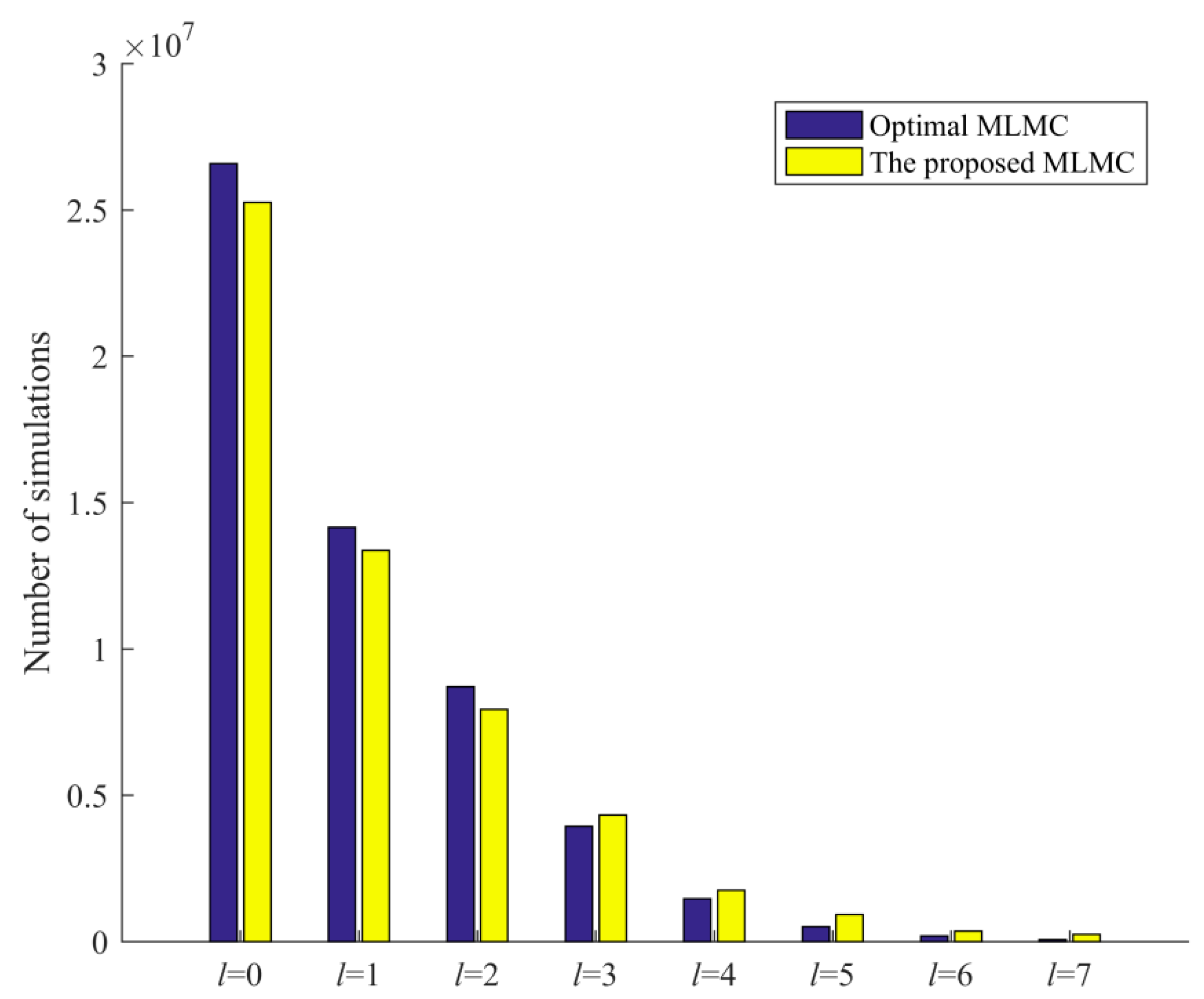
According to the theory of MLMC, information about P^(l) (or $P_{\mathrm{f},\mathrm{c}}^{(l)}(0,T)$, l = 0, …, L) is needed to optimize the number of random simulations allocated to each level of MLMC. However, the information is unavailable in advance. Thus, we propose a method in Section 3.2 to pre-estimate P^(l). Based on the pre-estimate, the computational cost of crude MCS and MLMC is compared and the size of random population MLMC allocates to each level l is optimized. Therefore, in order to validate the effectiveness of the proposed procedure, crude MCS, the proposed MLMC and the optimal MLMC in terms of total number of function evaluations are also compared by Figure 4, and the numbers of random simulations on each level determined according to the proposed procedure and the optimal MLMC are depicted by Figure 5. Figure 4 indicates that the optimal MLMC and the proposed MLMC are remarkably more efficient than crude MCS. The total number of function evaluations of the proposed method does not significantly increase with K, whereas that of crude MCS linearly increases with K. According to Figure 5, the computational cost allocated according to the proposed procedure is very close to that of the optimal MLMC, i.e., the true optimal allocation.

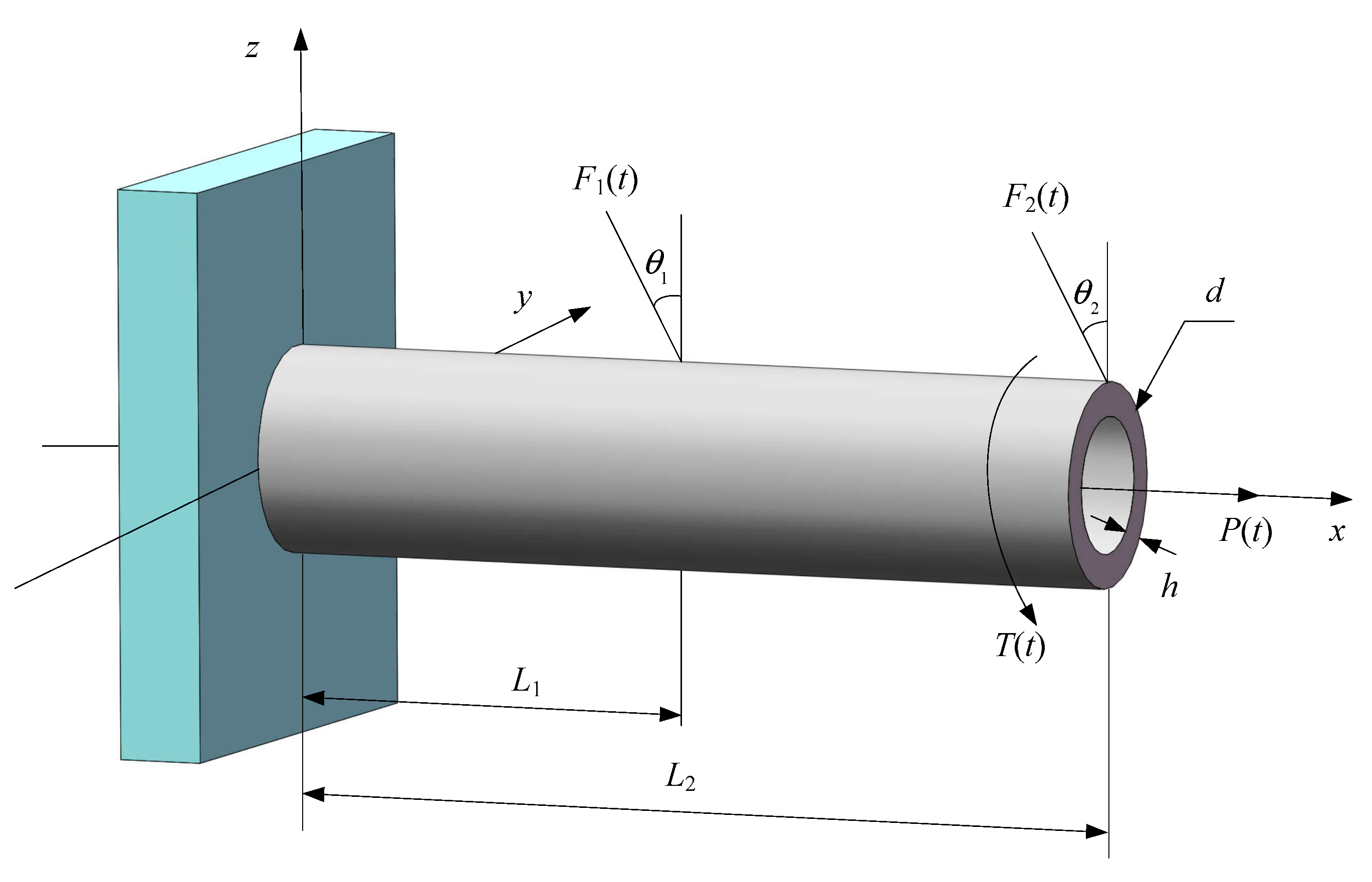
4.2. A Cantilever Tube Structure

The second example studies the cantilever tube structure shown by Figure 6. Four time-variant loads, i.e., F₁(t), F₂(t), P(t) and T(t), are applied to the structure. The yield strength of the structure linearly decreases with time caused by material degradation. The performance function is defined as:

$$G(\mathit{X},\mathit{Z}(t),t)={\sigma }_u(t)-\sqrt{{\sigma }_x^2(t)+3{\tau }_{zx}^2(t)}$$

(32)

where

$$\begin{array}{c}{\sigma }_x(t)=\frac{F_1(t)\sin ({\theta }_1)+F_2(t)\sin ({\theta }_2)+P(t)}{A}+\frac{M(t)d}{2I}\hfill \\ {\tau }_{zx}(t)=\frac{T(t)d}{4I}\hfill \\ M(t)=F_1(t)\cos ({\theta }_1)L_1+F_2(t)\cos ({\theta }_2)L_2\hfill \\ A=\frac{\pi }{4}[d^2-{(d-2h)}^2]\hfill \\ I=\frac{\pi }{64}[d^4-{(d-2h)}^4]\hfill \end{array}$$

X = [d, h, σ₀]^T and Z(t) = [F₁(t), F₂(t), T(t), P(t)]^T. The time interval of interest is [0, 5 year]. Input parameters are listed in

Table 3. The input parameters (example 2).

Variable	Distribution	Mean	Standard Deviation	Autocorrelation Coefficient Function
F1(t) (N)	Gaussian process	1800	180	$\exp (-|t_2-t_1|/4)$
F2(t) (N)	Gaussian process	1800	180	$\exp (-|t_2-t_1|)$
T(t) (Nm)	Gaussian process	1900	190	$\exp (-4{(t_2-t_1)}^2)$
P(t) (N)	Gaussian process	1800	180	$\exp (-4|t_2-t_1|)$
d (mm)	Normal	42	0.5	-
h (mm)	Normal	5	0.1	-
σ0 (MPa)	Normal	560	56	-
L1 (mm)	Deterministic	60	-	-
L2 (mm)	Deterministic	120	-	-
θ1 (°)	Deterministic	10	-	-
θ2 (°)	Deterministic	5	-	-

.

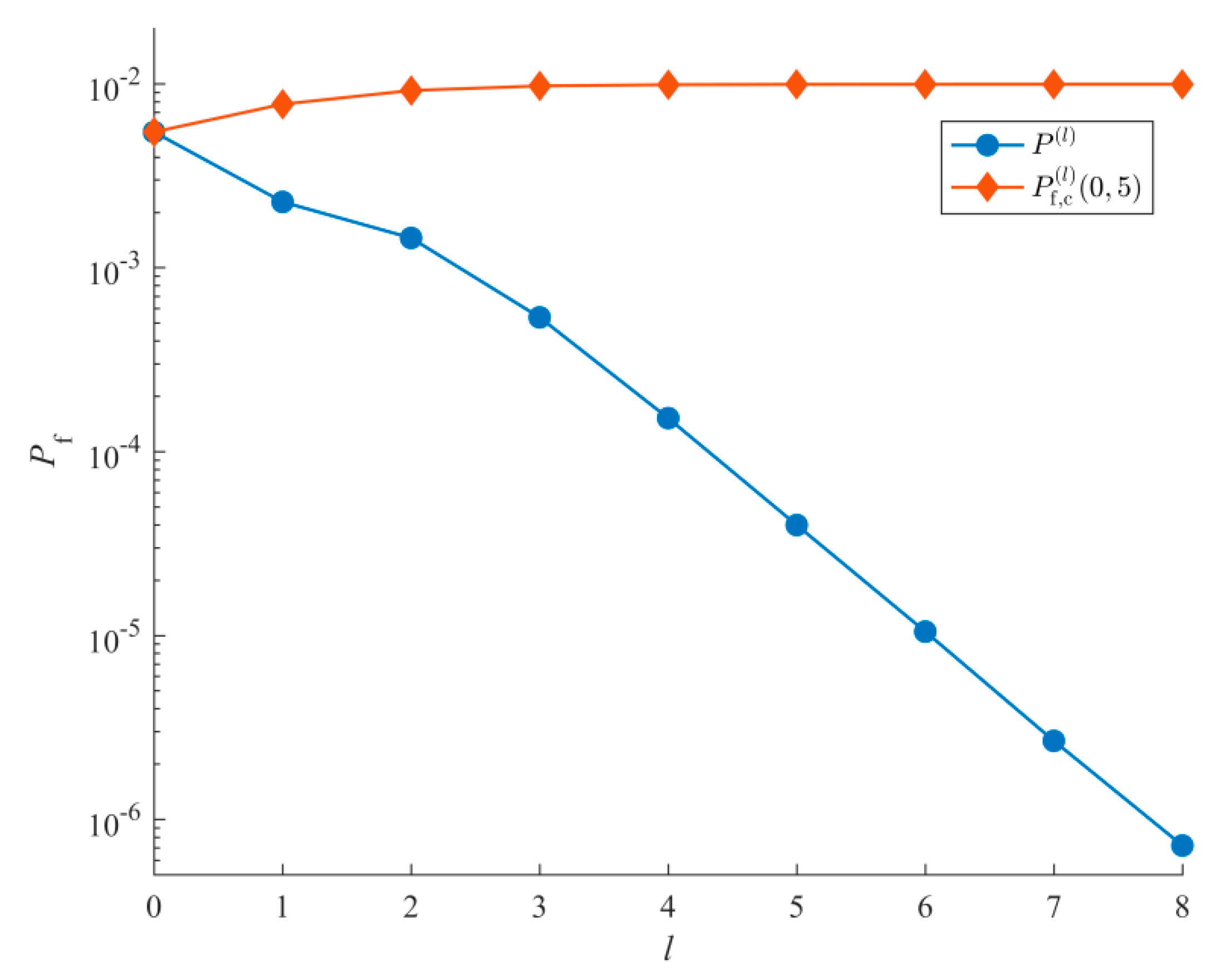
The benchmark values of P^(l) and $P_{\mathrm{f},\mathrm{c}}^{(l)}(0,T)$ (K₀ = 5 and l = 8) are calculated by crude MCS with 10⁸ random simulations, which is shown by Figure 7and

Table 4. Results of example 2.

K	δPf	K0	Method	${\widehat{\mathit{P}}}_{\mathbf{f},\mathbf{c}}$	Ncall	δ
640	-	-	Benchmark	9.933 × 10−3	-	1.0 × 10−3
	0.05	-	Crude MCS	1.03 × 10−2	2.49 × 107	4.97 × 10−2
		5	The proposed method	1.05 × 10−2	3.59 × 106	4.95 × 10−2
		10		9.80 × 10−3	4.60 × 106	4.94 × 10−2
		20		9.61 × 10−3	4.26 × 106	4.91 × 10−2
		40		9.36 × 10−3	5.42 × 106	4.95 × 10−2
		80		1.04 × 10−2	5.16 × 106	5.0 × 10−2
640	0.1	10	Crude MCS	9.90 × 10−3	6.67 × 106	9.80 × 10−3
			The proposed method	1.06 × 10−2	1.14 × 106	8.49 × 10−2
	0.05		Crude MCS	1.03 × 10−2	2.49 × 107	4.97 × 10−2
			The proposed method	9.80 × 10−3	4.60 × 106	4.94 × 10−2
	0.03		Crude MCS	1.01 × 10−2	7.1 × 107	2.98 × 10−2
			The proposed method	1.03 × 10−2	1.28 × 107	2.89 × 10−2
	0.01		Crude MCS	9.98 × 10−3	6.42 × 108	9.95 × 10−3
			The proposed method	9.94 × 10−3	1.42 × 108	9.40 × 10−3
320	0.05	10	Benchmark	9.931 × 10−3	-	1.0 × 10−3
			Crude MCS	1.01 × 10−2	1.27 × 107	4.97 × 10−2
			The proposed method	1.02 × 10−2	3.40 × 106	4.98 × 10−2
640			Benchmark	9.933 × 10−3	-	2.8 × 10−3
			Crude MCS	1.03 × 10−2	2.49 × 107	4.97 × 10−2
			The proposed method	9.80 × 10−3	4.60 × 106	4.94 × 10−2
1280			Benchmark	9.934 × 10−3	-	1.0 × 10−3
			Crude MCS	9.92 × 10−3	5.03 × 107	5.0 × 10−2
			The proposed method	1.037 × 10−2	8.41 × 106	4.86 × 10−2

. According to Figure 3 in Section 4.1 and Figure 7, P^(l) with smaller l (e.g., l < 5) contributes most of the cumulative probability of failure $P_{\mathrm{f},\mathrm{c}}^{(L)}(0,T)$. Considering that the computational cost on lower levels is much less than that on the highest level, optimizing the allocation of the computational cost is necessary in order to reduce the variance of MCS in a way that minimizes the over computational cost, which is exactly the purpose of the proposed procedure.

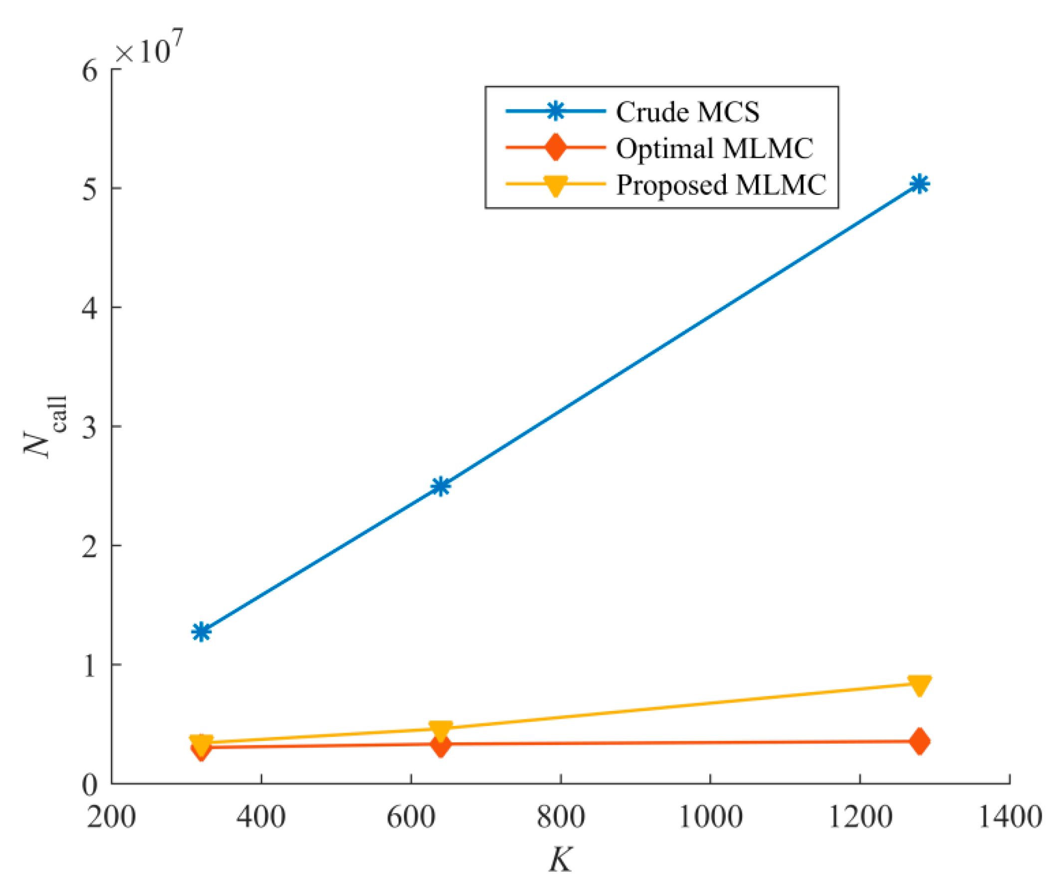
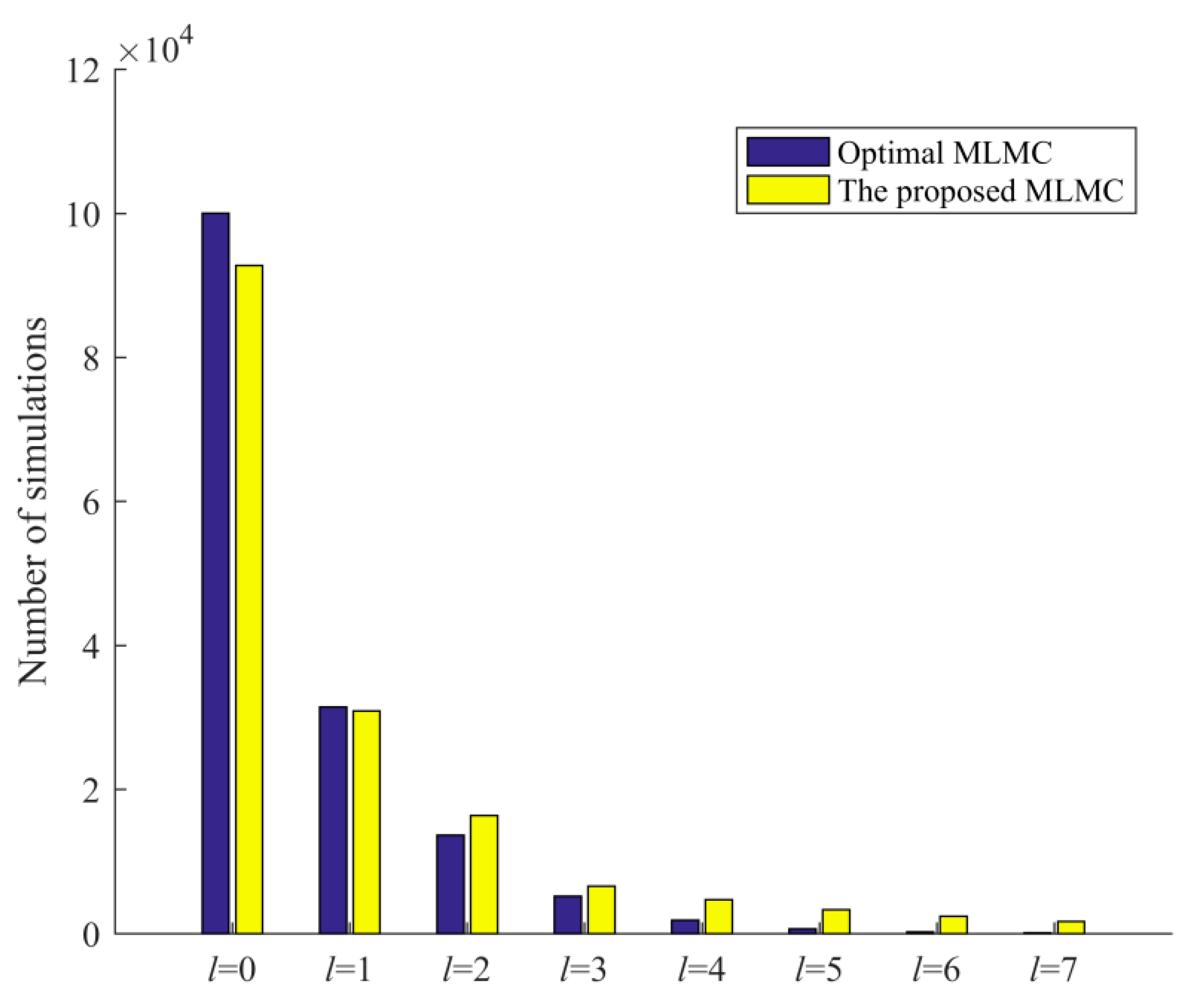
The performance of the proposed method considering different combinations of (K, δ_Pf, K₀) is investigated and compared to crude MCS. Results are summarized in Table 4. It can be noticed from Table 4 that achieving similar levels of accuracy, the proposed method needs significantly less evaluations of performance function than crude MCS. The saving of the proposed method increases with the accuracy requirement (small δ_Pf means high accuracy requirement). Figure 8 compares crude MCS, the proposed MLMC and the optimal MLMC. It shows that MLMCs hold considerable advantage over crude MCS in terms of computational cost. The allocation of computational cost determined according to the proposed method is near to that of the optimal MLMC, which is concluded from Figure 9.

5. Conclusions

This paper presents a random simulation method called MLMC for TRA to enhance the efficiency of MCS. The proposed method discretizes the time interval of interest using a geometric sequence of timesteps and then estimates the cumulative probability of failure $P_{\mathrm{f},\mathrm{c}}^{(L)}(0,T)$ (Equation (17)) associated with the finest level by computing corrections P^(l) (Equations (17) and (19)) coming from all levels. Considering the computational complexity of each level (C_l, Equation (27)) and the contribution that each P^(l) makes to $P_{\mathrm{f},\mathrm{c}}^{(L)}(0,T)$, the allocation of computational cost is optimized (Equation (26)).

In the proposed procedure of MLMC, the switch between MLMC and crude MCS is proposed, which is merely to circumvent the complex deduction of conditions that MLMC is more efficient than crude MCS. The switch performs practically no function in Section 4 because all pre-estimates of the computational cost of crude MCS and MLMC show that MLMC needs less function evaluations, which indicates that MLMC is commonly more efficient. As the random trajectories of the time-variant performance function are generated in the same way with crude MCS, the proposed method retains most of the characteristics of robustness with respect to nonlinearity and dimensions of performance function. However, since a geometric sequence of different timesteps is essential for the proposed methods, the number of discretized time instants is limited by K₀ and L (Equation (4)).

The effectiveness of the proposed method is validated by two examples. Results demonstrate that the proposed method remarkably reduces the total number of function evaluations while maintaining the accuracy, meeting the prescribed requirement. The saving increases with the accuracy requirement. Moreover, results indicate that the total number of function evaluations of the proposed method increases slowly with K. This characteristic means that one can use large K to reduce the discretization error (Equation (10)) without a significant increase in the computational cost, like crude MCS. The proposed method can be combined, in principle, with surrogate models (e.g., the Kriging model and polynomial chaos expansion) and variance reduction techniques (e.g., IS and SS for TRA) to obtain great savings.

References

- Straub, D.; Schneider, R.; Bismut, E.; Kim, H.J. Reliability analysis of deteriorating structural systems. Struct. Saf. 2020, 82, 101877. [Google Scholar] [CrossRef]
- Tian, H.; Chen, Y.L.; Li, F.Y. A Novel Approach to Evaluate the Time-Variant System Reliability of Deteriorating Concrete Bridges. Math. Probl. Eng. 2015, 2015, 129787. [Google Scholar] [CrossRef] [Green Version]
- Zio, E.; Pedroni, N. How to effectively compute the reliability of a thermal-hydraulic nuclear passive system. Nucl. Eng. Des. 2011, 241, 310–327. [Google Scholar] [CrossRef] [Green Version]
- Honfi, D. Time-variant reliability of timber beams according to Eurocodes considering long-term deflections. Wood Mater. Sci. Eng. 2020, 15, 250–260. [Google Scholar] [CrossRef]
- Rackwitz, R. Reliability analysis—a review and some perspectives. Struct. Saf. 2001, 23, 365–395. [Google Scholar] [CrossRef]
- Hu, Z.; Du, X.P. Time-dependent reliability analysis with joint upcrossing rates. Struct. Multidiscip. Optim. 2013, 48, 893–907. [Google Scholar] [CrossRef]
- Andrieu-Renaud, C.; Sudret, B.; Lemaire, M. The PHI2 method: A way to compute time-variant reliability. Reliab. Eng. Syst. Saf. 2004, 84, 75–86. [Google Scholar] [CrossRef]
- Breitung, K. Asymptotic crossing rates for stationary Gaussian vector processes. Stoch. Process. Appl. 1988, 29, 195–207. [Google Scholar] [CrossRef] [Green Version]
- Li, J.; Chen, J.; Chen, Z. Developing an improved composite limit state method for time-dependent reliability analysis. Qual. Eng. 2020, 32, 298–311. [Google Scholar] [CrossRef]
- Hu, Y.; Lu, Z.; Wei, N.; Zhou, C. A single-loop Kriging surrogate model method by considering the first failure instant for time-dependent reliability analysis and safety lifetime analysis. Mech. Syst. Signal Process. 2020, 145, 106963. [Google Scholar] [CrossRef]
- Du, W.; Luo, Y.; Wang, Y. Time-variant reliability analysis using the parallel subset simulation. Reliab. Eng. Syst. Saf. 2019, 182, 250–257. [Google Scholar] [CrossRef]
- Singh, A.; Mourelatos, Z.P.; Nikolaidis, E. Time-Dependent Reliability of Random Dynamic Systems using Time-Series Modeling and Importance Sampling. SAE Int. J. Mater. Manuf. 2011, 4, 929–946. [Google Scholar] [CrossRef]
- Sudret, B. Analytical derivation of the outcrossing rate in time-variant reliability problems. Struct. Infrastruct. Eng. 2008, 4, 353–362. [Google Scholar] [CrossRef]
- Jiang, C.; Huang, X.P.; Han, X.; Zhang, D.Q. A Time-Variant Reliability Analysis Method Based on Stochastic Process Discretization. J. Mech. Des. 2014, 136, 091009. [Google Scholar] [CrossRef]
- Gong, C.Q.; Frangopol, D.M. An efficient time-dependent reliability method. Struct. Saf. 2019, 81, 101864. [Google Scholar] [CrossRef]
- Yu, S.; Zhang, Y.; Li, Y.; Wang, Z. Time-variant reliability analysis via approximation of the first-crossing PDF. Struct. Multidiscip. Optim. 2020, 62, 2653–2667. [Google Scholar] [CrossRef]
- Jiang, C.; Wei, X.P.; Wu, B.; Huang, Z.L. An improved TRPD method for time-variant reliability analysis. Struct. Multidiscip. Optim. 2018, 58, 1935–1946. [Google Scholar] [CrossRef]
- Zhang, Y.W.; Gong, C.L.; Li, C.N. Efficient time-variant reliability analysis through approximating the most probable point trajectory. Struct. Multidiscip. Optim. 2020, 63, 289–309. [Google Scholar] [CrossRef]
- Yu, S.; Wang, Z.L. A Novel Time-Variant Reliability Analysis Method Based on Failure Processes Decomposition for Dynamic Uncertain Structures. J. Mech. Des. 2018, 140, 051401. [Google Scholar] [CrossRef]
- Kamiński, M. The Stochastic Perturbation Method for Computational Mechanics; John Wiley & Sons: Chichester, UK, 2013. [Google Scholar]
- Singh, A.; Mourelatos, Z.P.; Li, J. Design for Lifecycle Cost Using Time-Dependent Reliability. J. Mech. Des. 2010, 132, 091008. [Google Scholar] [CrossRef]
- Mourelatos, Z.P.; Majcher, M.; Pandey, V.; Baseski, I. Time-Dependent Reliability Analysis Using the Total Probability Theorem. J. Mech. Des. 2015, 137, 031405. [Google Scholar] [CrossRef]
- Ping, M.H.; Han, X.; Jiang, C.; Xiao, X.Y. A time-variant extreme-value event evolution method for time-variant reliability analysis. Mech. Syst. Signal Process. 2019, 130, 333–348. [Google Scholar] [CrossRef]
- Hu, Z.; Mahadevan, S. A Single-Loop Kriging Surrogate Modeling for Time-Dependent Reliability Analysis. J. Mech. Des. 2016, 138, 061406. [Google Scholar] [CrossRef]
- Yang, D.Y.; Teng, J.G.; Frangopol, D.M. Cross-entropy-based adaptive importance sampling for time-dependent reliability analysis of deteriorating structures. Struct. Saf. 2017, 66, 38–50. [Google Scholar] [CrossRef]
- Singh, A.; Mourelatos, Z.P.; Nikolaidis, E. An Importance Sampling Approach for Time-Dependent Reliability. IDETC-CIE 2011, 5, 1077–1088. [Google Scholar] [CrossRef]
- Sonal, S.D.; Ammanagi, S.; Kanjilal, O.; Manohar, C.S. Experimental estimation of time variant system reliability of vibrating structures based on subset simulation with Markov chain splitting. Reliab. Eng. Syst. Saf. 2018, 178, 55–68. [Google Scholar] [CrossRef]
- Kurtz, N.; Song, J. Cross-entropy-based adaptive importance sampling using Gaussian mixture. Struct. Saf. 2013, 42, 35–44. [Google Scholar] [CrossRef]
- Ching, J.; Au, S.K.; Beck, J.L. Reliability estimation for dynamical systems subject to stochastic excitation using subset simulation with splitting. Comput. Methods Appl. Mech. Eng. 2005, 194, 1557–1579. [Google Scholar] [CrossRef]
- Wang, Z.L.; Mourelatos, Z.P.; Li, J.; Baseski, I.; Singh, A. Time-Dependent Reliability of Dynamic Systems Using Subset Simulation With Splitting Over a Series of Correlated Time Intervals. J. Mech. Des. 2014, 136, 061008. [Google Scholar] [CrossRef] [Green Version]
- Wang, Z.; Liu, J.; Yu, S. Time-variant reliability prediction for dynamic systems using partial information. Reliab. Eng. Syst. Saf. 2020, 195, 106756. [Google Scholar] [CrossRef]
- Hawchar, L.; El Soueidy, C.P.; Schoefs, F. Global kriging surrogate modeling for general time-variant reliability-based design optimization problems. Struct. Multidiscip. Optim. 2018, 58, 955–968. [Google Scholar] [CrossRef]
- Hu, Z.; Du, X.P. Mixed Efficient Global Optimization for Time-Dependent Reliability Analysis. J. Mech. Des. 2015, 137, 051401. [Google Scholar] [CrossRef]
- Hawchar, L.; El Soueidy, C.-P.; Schoefs, F. Principal component analysis and polynomial chaos expansion for time-variant reliability problems. Reliab. Eng. Syst. Saf. 2017, 167, 406–416. [Google Scholar] [CrossRef]
- Hawchar, L. Time-variant reliability analysis using polynomial chaos expansion. In Proceedings of the 12th International Conference on Applications of Statistics and Probability in Civil Engineering, ICASP12, Vancouver, BC, Canada, 12–15 July 2015. [Google Scholar]
- Yan, Y.; Wang, J.; Zhang, Y.; Sun, Z. Kriging Model for Time-Dependent Reliability: Accuracy Measure and Efficient Time-Dependent Reliability Analysis Method. IEEE Access 2020, 8, 172362–172378. [Google Scholar] [CrossRef]
- Wang, D.; Jiang, C.; Qiu, H.; Zhang, J.; Gao, L. Time-dependent reliability analysis through projection outline-based adaptive Kriging. Struct. Multidiscip. Optim. 2020, 61, 1453–1472. [Google Scholar] [CrossRef]
- Jiang, C.; Wang, D.P.; Qiu, H.B.; Gao, L.; Chen, L.M.; Yang, Z. An active failure-pursuing Kriging modeling method for time-dependent reliability analysis. Mech. Syst. Signal Process. 2019, 129, 112–129. [Google Scholar] [CrossRef]
- Giles, M.B. Multilevel Monte Carlo path simulation. Oper. Res. 2008, 56, 607–617. [Google Scholar] [CrossRef] [Green Version]
- Allaix, D.L.; Carbone, V.I. An efficient coupling of FORM and Karhunen-Loeve series expansion. Eng. Comput. 2016, 32, 1–13. [Google Scholar] [CrossRef]
- Yang, L.; Gurley, K.R. Efficient stationary multivariate non-Gaussian simulation based on a Hermite PDF model. Probabilistic Eng. Mech. 2015, 42, 31–41. [Google Scholar] [CrossRef]
- Li, C.; Der Kiureghian, A. Optimal Discretization of Random Fields. J. Eng. Mech. 1993, 119, 1136–1154. [Google Scholar] [CrossRef]
Figure 1.
Flowchart of the proposed multilevel Monte Carlo (MLMC).
Figure 2.
The steel bending beam (example 1).
Figure 3.
P(l) and of the steel bending beam. l = 0 and 8 corresponds to K = 5 and 1280, respectively. According to Equation (17), .
Figure 4.
The change of computational cost with K. Crude MCS, the optimal MLMC and the proposed method are compared with δPf = 0.03 and K0 = 10. The optimal MLMC denotes the MLMC method whose computational cost is optimized according to Equations (25)–(27) using P(l) (l = 0, …, L) shown in Figure 3. Since P(l) is unavailable in practice, the computational cost of the optimal MLMC is theoretically minimum for MLMC.
Figure 5.
The allocation of computational cost determined by the optimal MLMC and the proposed method ((K, δPf, K0) = (1280, 0.03,10)).
Figure 6.
The cantilever tube structure (example 2).
Figure 7.
P(l) and of example 2. l = 0 and 8 corresponds to K = 5 and 1280, respectively.
Figure 8.
The change of computational cost with K (δPf = 0.05 and K0 = 10).
Figure 9.
The allocation of computational cost determined by the optimal and the proposed method ([K, δPf, K0] = [1280, 0.05,10]).