Article

Hydro-Mechanical Effects of Several Riparian Vegetation Combinations on the Streambank Stability—A Benchmark Case in Southeastern Norway

Natural Hazards Division, Norwegian Geotechnical Institute (NGI), 0806 Oslo, Norway
*
Author to whom correspondence should be addressed.
Sustainability 2021, 13(7), 4046; https://0-doi-org.brum.beds.ac.uk/10.3390/su13074046
Submission received: 8 March 2021 / Revised: 1 April 2021 / Accepted: 2 April 2021 / Published: 6 April 2021

Abstract

:
Vegetation can be used as a nature-based solution (NBS) to restore rivers and mitigate water-triggered processes along streambanks. Roots are well known to improve the overall stability of slopes through hydro-mechanical reinforcement within the rooted zone. Vegetation-based solutions require the selection of species that are most suitable for specific locations, and they are aimed at restoring the natural state and function of river systems in support of biodiversity, flood management, and landscape development. Selecting a combination of different species along different zones of the riverbank can improve the conditions for the river system with regard to biodiversity and stability. Therefore, more studies are needed to investigate how the combination of a variety of different plant species can improve the stability of the riverbank. This paper presents a methodological approach for slope stability modeling including vegetation as well as the results obtained from a series of slope stability calculations adopting the proposed methodology. The analyses were carried out for critical shallow (≤3 m deep) shear planes of ideal benchmark slopes covered with four different plant combinations—(i) only grass, (ii) grass and shrubs, (iii) only trees, and (iv) trees, shrubs, and grass—for species typically found along streams in southeastern Norway. In this desk study, two types of tree species were selected, namely Norway spruce (Picea abies) and Downy birch (Betula pubescens). The Goat willow (Salix caprea) was selected as a shrub, while a common mixed-grass was chosen as grass. Vegetation features were obtained from the literature. The methodology was used for two main cases: (1) considering only the mechanical contribution of vegetation and (2) considering both the hydrological and mechanical reinforcement of vegetation. The main outcome of the numerical modeling showed that the purely mechanical contribution of vegetation to slope stability could not be decoupled from the hydrological reinforcement in order to have a realistic assessment of the roots improvement to the stability. The most critical shear surfaces occurred below the rooted zone in all cases, and the best performance was obtained using the combinations including trees. Considering the typical climate conditions in Norway, the hydro-mechanical reinforcement was most effective in the spring and for combinations including low height vegetation (i.e., grass and shrubs). The study concludes that a mixed combination of vegetation (trees, shrubs, and grass) is the most suitable for reaching the highest hydro-mechanical reinforcement of streambanks, together with erosion protection and boosting the ecosystem biodiversity. The current study can help practitioners determine which vegetation cover combination is appropriate for improving the current stability of a streambank with restoration practices.

1. Introduction

Climate change and loss of biodiversity are currently two big challenges the modern world faces [1]. The future climate of Norway and the Nordic countries is forecasted to be warmer, wetter, and more erratic with respect to freeze–thaw and wetting–drying cycles [2]. Therefore, events triggered by water, such as erosion, floods, and landslides, are expected to become more frequent in the future. Areas along rivers and streams are particularly vulnerable to impacts of climate change.
Riverbanks can be considered as a type of slope, and as such, their stability is based on the same principles that govern the stability of hill slopes and embankments. Hence, the assessment of the factor of safety (FS) as an indicator of the riverbank stability is widely accepted in the geotechnical engineering practice. Factor of safety is defined as the ratio of the shear strength (resistance) along a potential failure surface to the driving force resulting from the integration of shear stresses acting on that surface. A value of FS greater than unity means that the slope is stable.
However, the vulnerability of riverbanks and streambanks to slope instability is not only attributable to the effects of the climate change but also to the lack of vegetation in the proximity of the banks. Some studies conducted in Australia have demonstrated that forested banks or banks with well-established vegetation were considerably more stable than banks with similar topography that were subjected to vegetation clearing in the past [3].
Due to unfavorable conditions for agriculture in large parts of Norway, the cultivation of new lands for increasing grain producing areas took place in the 1970s in many areas. As a result of this, ravines and steep lands were made suitable for modern machinery by leveling, meandering creeks were straightened, and vegetation zones between agricultural lands and creeks were reduced or removed [4].
Apart from the well-known effects in reducing surface erosion, riparian vegetation also provides hydrological and mechanical reinforcement to bank stability [5]. Hence, native plants can be used as a nature-based solution (NBS) to reduce the risk of bank instability and simultaneously regenerate and preserve the complex variety of in-stream and riverside habitats.
In partially saturated slopes, the hydrological effect of plants on soil shear strength is mostly given by a reduction of the pore-water pressure and the resulting increase of soil suction through water extraction, but this effect is often ignored in slope stability problems. Soil–water dynamics influenced by the presence of roots are the root water uptake from the soil and the stemflow [6], which are all processes needed by the plants to transfer the water from the soil to the structure, to be able to exert its vital functions. They are influenced by the roots and shoot characteristics [7,8,9], tree architecture, seasonality, and meteorological conditions [7]. All these processes that resulted in an increment of soil suction have proven beneficial to slope stability [10]. Furthermore, recent studies have shown that also the soil’s hydrological regime may influence on the overall soil–root reinforcement [11].
Mechanical reinforcement from root shear resistance is generally accepted to be included as additional cohesion, which is a function of the strength of the roots crossing potential shear planes, and the number and diameter of such roots [12], for most soils. Some exceptions were observed for coarse soils, where roots have demonstrated to also increase the friction angle of the composite material [11,13]. Attempts to estimate the hydro-mechanical effects of vegetation on riverbank and slope stability have been conducted [3,14,15,16] using either less or more accurate root models: the first considering an additional cohesion exerted by the roots in the case of single instance root breaking, and the latter considering progressive root breaking during soil shearing. One of the main conclusions was that root models using a single instance of root breaking tend to overestimate the overall effect of roots on slope stability; thus, the use of a progressive root-breaking model to quantify the roots reinforcement is more realistic [15].
How the combination of different native plant species can improve the stability of the streambank needs to be further studied, so that both geotechnical and ecological considerations are evaluated when it comes to selecting the best vegetation combination as NBS along riverbanks. This paper contributes to the research on this topic by analyzing benchmark cases representative of streambanks found in southeastern Norwegian catchments. To assess the role of combined vegetation on streambanks, an ideal slope is analyzed, and the most common among the native tree, shrub, and grass species are considered.

2. Materials and Methods

2.1. Vegetation Species Selected in This Study

Species that can be used as NBS are highly dependent on local conditions, such as local climate as well as soil and groundwater conditions.
Plant species that could thrive on streambanks were selected based on native vegetation commonly found in southeastern Norwegian ravines. Although this was a desk study that did not involve field experiments, the authors selected a study area in Åserud ravine in Nes municipality in southeastern Norway and therefore investigated plant species registered in that specific area (BioFokus, 2016 and https://www.artsdatabanken.no/, access date 1 October 2020). This particular ravine consists of a meandering stream below marine limit that enters Glomma river (Figure 1).
The geology of the area consists mainly of a mix of marine and stream/fluvial deposits. According to the Köppen–Geiger climate classification [17], the climate type is classified as Dfb—Warm-summer humid continental climate, with climate cold and temperate and with the highest precipitation in the summer–fall season.
Hydrological factors that can cause the triggering of instabilities in these ravines are prolonged rainfall or snow melt. The period of the year where these triggering hydrological factors are prevalent ranges from spring to autumn, when the ground is unfrozen and rainfall and snow melt can both lead to water infiltration into the soil and river flooding.
Surrounding the ravine are agricultural lands and grazing fields, which could imply a contribution of pollutants and increased values of phosphate to the ravine. Therefore, selecting species living here could also be of future use for studies regarding improving water quality, nature restoration, etc. Two types of tree species were selected: Norway spruce (Picea abies), called here T1, and Downy birch (Betula pubescens), T2. The Goat willow (Salix caprea), which is also called S. Willow, was selected as the shrub. It grows in the woods in almost all of Norway and can occur both as a small tree (with one larger main stem) and a bush (several stems of similar size) depending on growth conditions. Examples of ravine conditions found in southeastern Norway are provided in Figure 2.
A summary of the tree and shrub features and the environmental conditions where they grow, based on a report provided by [18] for Norwegian ravines, is shown in Table 1. For the grass species (G), mixed grass was chosen based on a previous study conducted along a Norwegian catchment by [19].

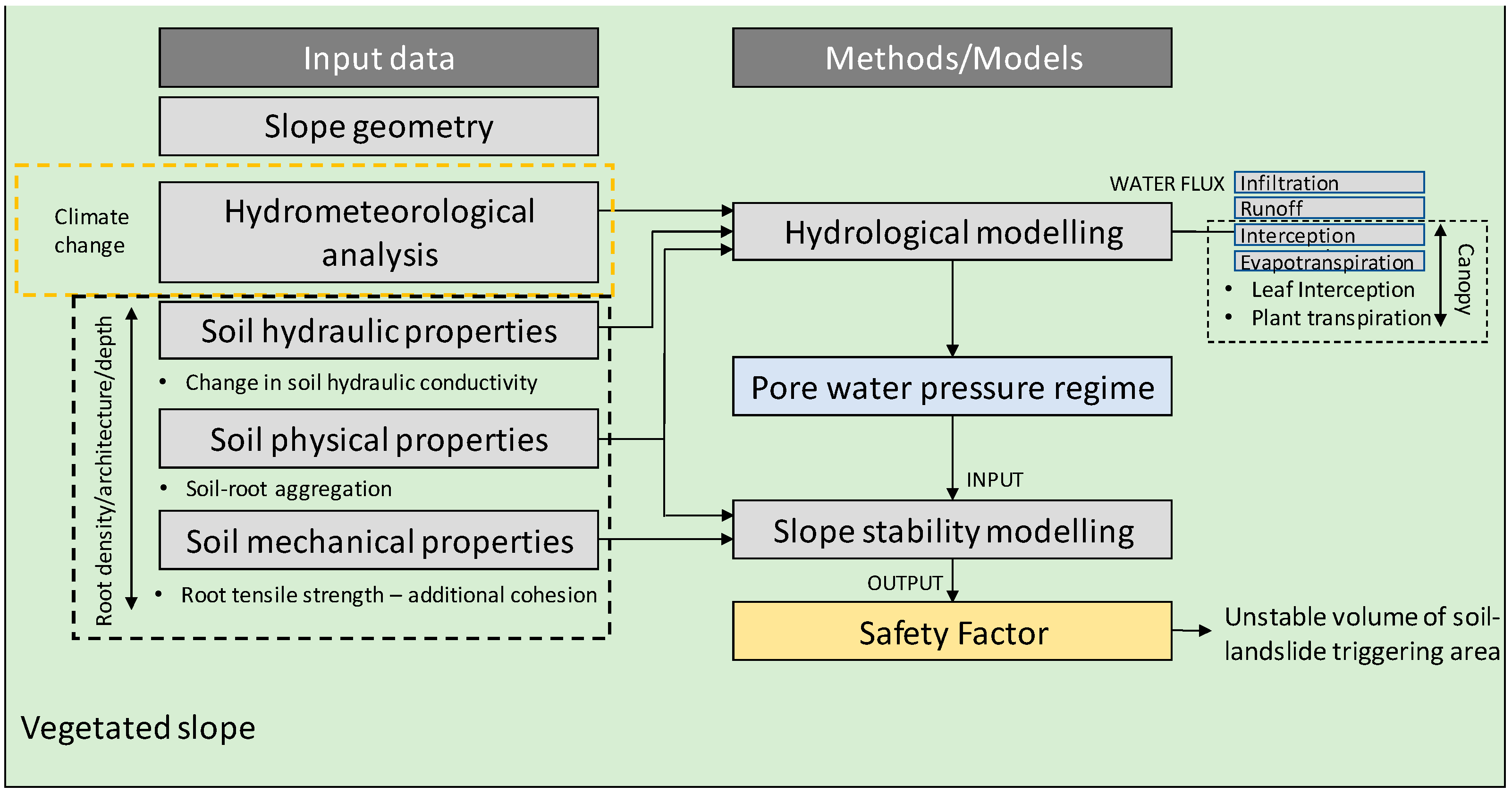
2.2. Modeling of Slope Stability Using Vegetation

Many factors need to be considered when assessing slope stability, including vegetation [20]. The methodological approach shown in Figure 3 can be adopted. This approach consists of two main parts:
  • Hydrological modeling, to assess the pore water pressure regime;
  • Slope stability modeling, to assess the safety factor.
As input data, hydrometeorological analysis implies the collection of meteorological data (e.g., rainfall intensity, wind, temperature, relative humidity), or the analysis of potential future climate scenarios, to be used to feed the hydrological model. For the input data related to the soil, many soil parameters as well as hydraulic processes (water fluxes) are affected by the presence of vegetation. An attempt to categorize the effects of vegetation on the input data has been done, based on whether they are a function of the root features (mostly density, architecture and depth) or the canopy (type of aboveground vegetation).
For the hydrological modeling and evaluation of the pore water pressure regime in the ground, both roots and aboveground vegetation features influence the processes and the soil parameters. The hydraulic conductivity of the soil strongly depends on the type (coarse or fine) and age (i.e., young or decaying) of roots. Some preliminary functions were proposed to model the effect of roots on the change of soil hydraulic conductivity, but so far, they have only been included in analytical analyses [21]. However, recent studies have found that hydraulic conductivity of the soil can also change with time as the roots develop and grow [22]. Additionally, as roots occupy the pores, they tend to change the soil void ratio and thus change the soil bulk density, while shear strength is mostly affected by the root diameter and depth [23].
With regard to the aboveground vegetation in a water flux, interception accounts for the rainwater intercepted by the vegetation that does not infiltrate into the soil. Interception is strongly affected by the canopy area and parameters such as the Leaf Area Index (LAI) [24], which is defined as the projected area of leaves over a unit of land. Most of the hydrological models calculate the potential evapotranspiration with the equation proposed by Penman–Monteith [25], in which the potential transpiration given by the vegetation is usually a function of the LAI and the soil cover fraction.
To assess the factor of safety associated with a root reinforced slope, the commercial software GeoStudio (GEO-SLOPE International, Ltd., Calgary, AL, Canadian) was used (2019 version), with packages SEEP/W and SLOPE/W. The module SEEP/W, using finite element (FEM)-based formulation to analyze groundwater seepage and excess pore-water pressure dissipation, was adopted for the hydrological modelling and the calculation of pore-water pressure distribution.
To simulate the change of soil water content, and thus pore-water pressure dissipation due to the transpiration of the roots, the module SEEP/W uses the modified Richard’s equation [26]:
θ t = z ( K ( h ) h z + K ( h ) ) S ( z , t )
where θ is the volumetric water content, h is the total hydraulic head, K(h) is the soil hydraulic conductivity, and S(z,t) is the Sink term, which can be explained as the volumetric water content taken by the roots during the transpiration process. This term depends on the initial water content, the root density with depth, and the plant moisture limit [27,28,29].
The initial water content is dependent on the location of the initial water table (WT). The plant moisture limit function used was the same for all types of species and was equal to 1 for values of suction between 1 and 100 kPa; then, it had a decreasing linear trend toward 0 for a suction value of 1500 kPa. This function gives an indication that plants can actively uptake water from the soil when the suction is below 100 kPa, whereas as the suction values increase (meaning the soil becomes drier), the ability of plants to uptake water is reduced.
The normalized root density was derived from root mass and volume data available in the literature for each species [21,30,31], and it ranged between 0 (no density) and 1 (maximum value of root mass).
More details on the equations used within SEEP/W can be found in [32].
The fluctuation of groundwater level in the streambanks is an aspect that strongly influences the pore water pressure distribution in the soil and consequently the slope stability. In this study, different initial levels of the water table were considered to investigate how the water table influences the stability of vegetated slopes. The water tables were selected based on the experience of the authors for conditions around the study area.
Following the SEEP/W analysis, the limit equilibrium method (LEM) within the SLOPE/W package was used for slope stability modeling and calculation of the safety factor assuming the rotational failure model proposed by Bishop [33]. The use of failure modes other than rotational to assess bank stability is still under debate, as banks can collapse by a variety of failure mechanisms. Simplified infinite slope stability models have been adopted in the past to account for the role of vegetation on the stability of forested plane slopes [34,35,36]. Other studies addressing the slope stability of streambanks have used the BSTEM—Bank-Stability and Toe-Erosion Model [36], which uses a wedge failure mechanism and is considered more appropriate when assessing the stability of frictional slopes [37]. The limitation of the current version of BSTEM model is that the root reinforcement is only designed and tested for top of bank vegetation, not vegetation covering an entire bank slope [19].
The GeoStudio software can create soil regions with different properties, not only at the top but also along the entire bank of the slope. Therefore, regions having the properties of the composite material made by soil permeated by roots were created along the surface of the slope. The depth of each vegetated region (i.e., composite material) was equal to the average depth of the roots of the plant species selected for this study (see Section 2.3.1).
The selected method to evaluate the role that vegetation plays in reinforcing the slope was to calculate the percentage of FS increment compared to the bare condition for each scenario. The FS increment was calculated using Equation (2):
F S   i n c r e m e n t   ( % ) =   Δ F s F S B · 100 =   ( F s V F S B ) F S B · 100
where FSB is the safety factor calculated for the condition of bare slope and ∆FS is the difference between FS of the vegetated combination (FSV) and the FS of the bare slope: (FSV − FSB). The bare slope condition is calculated for each scenario along with the vegetated combination, and therefore, the reference FS for bare soil changes in each increment calculation.

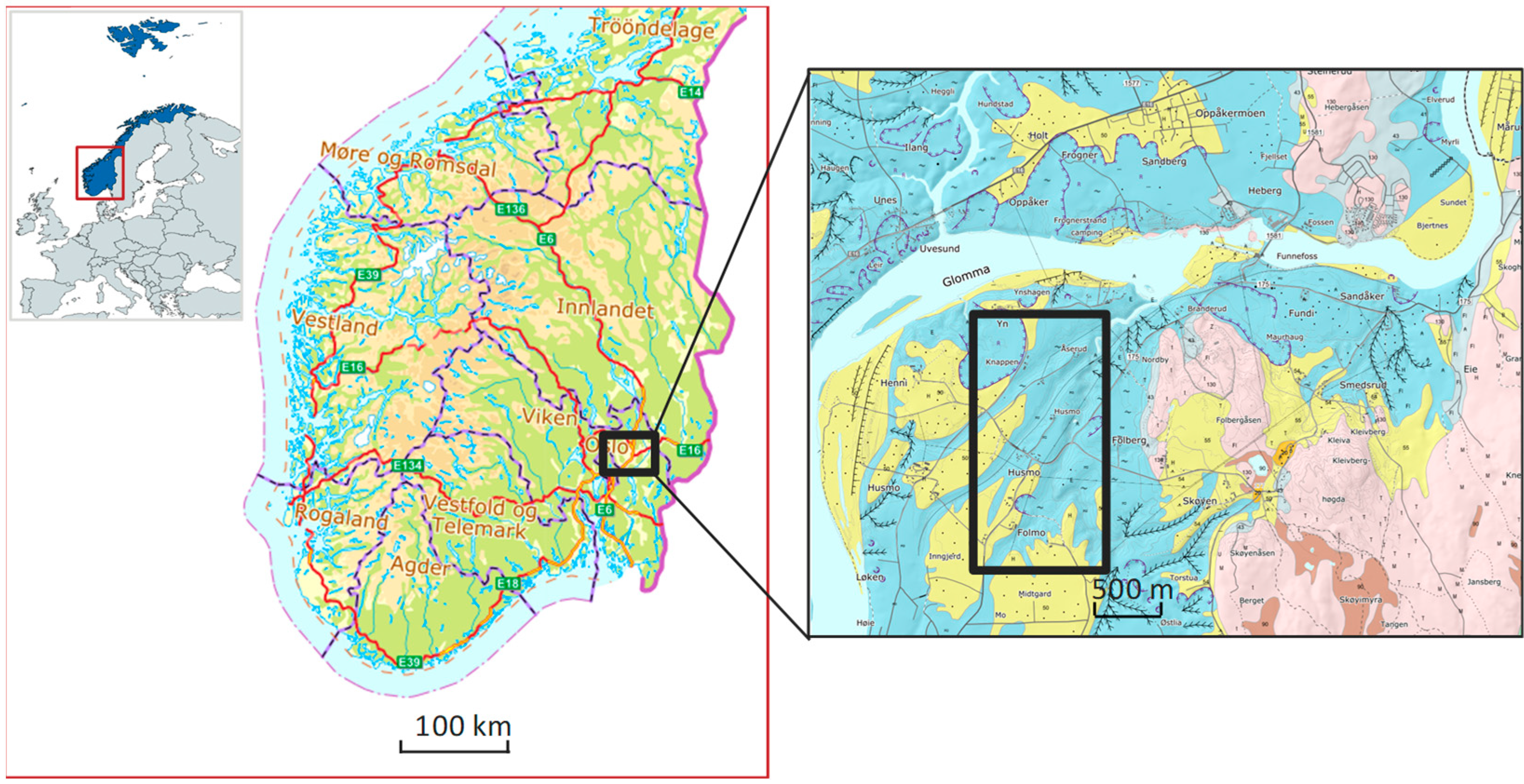
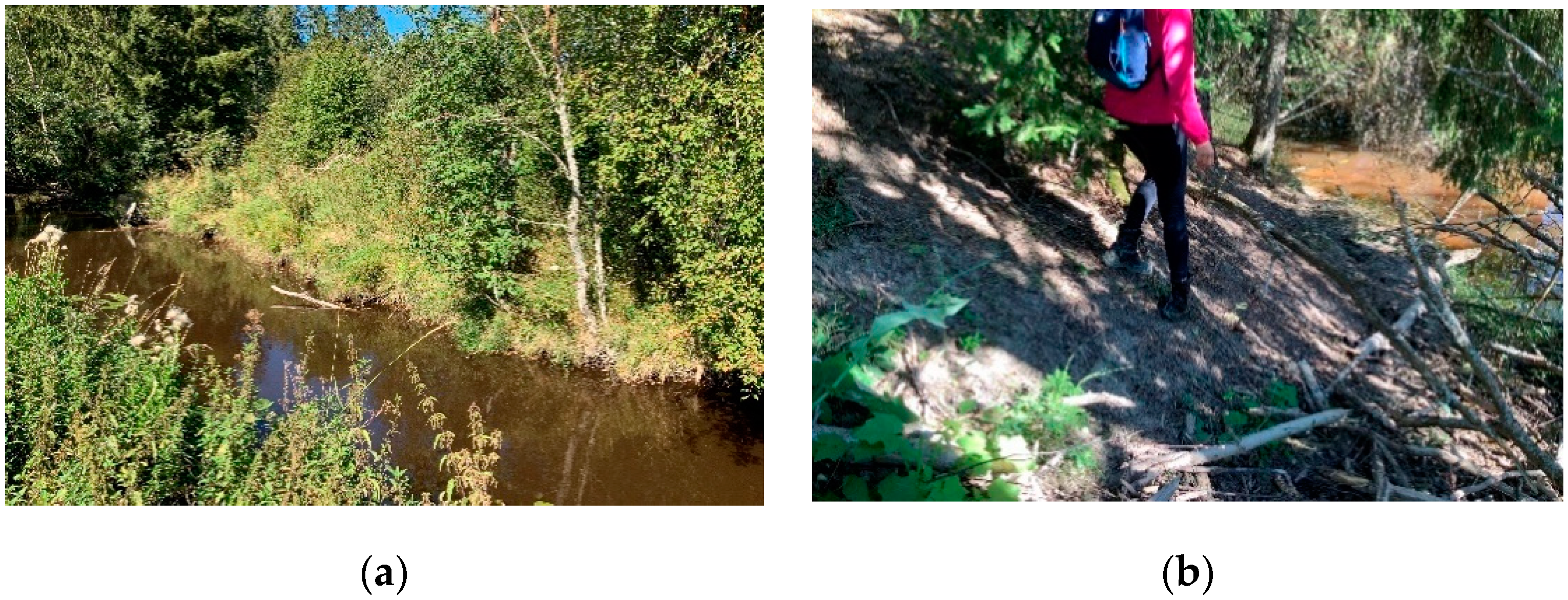
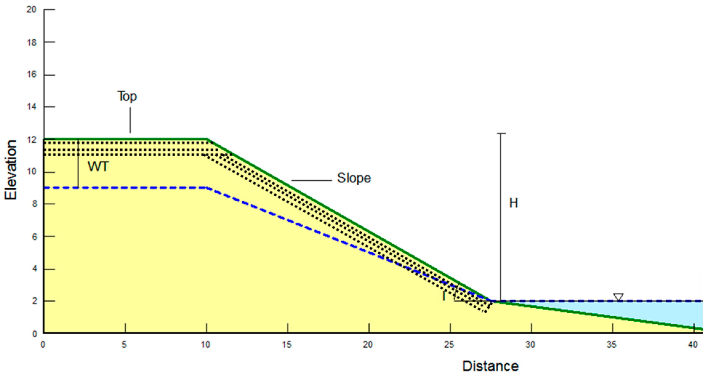
2.3. Benchmark Cases: Geometry, Initial Conditions, and Vegetation Combination

Ideal benchmark slopes with different inclination were analyzed. For simplicity, a homogeneous slope with a silty soil was considered in the analyses. It is worth mentioning that Norwegian ravines sometimes can be made of quick clay layers, which can collapse and behave as a flow-like material when disturbed, but the stability of this special soil goes beyond the scope of this study. Publicly available borehole information near the ravine shows a dry crust between 1 and 3 m thick overlying clayey material with varying degrees of silt. Some of the clay could possibly be quick clay. In this study, vegetation influences only the uppermost layers of soil, and failure surfaces that were maximum 3 m deep were selected for analysis. Although the site area may have clay deposits at depth, to simplify the model by only having one material type, a silty material was selected in Geostudio, which is more representative of the surficial materials that would be found in the ravine. The main soil properties chosen, the initial conditions of the water table, as well as the inclination of the slopes analyzed are listed in Table 2. Although the water level in the river affects slope stability, the level was considered constant for all analyses to minimize model complexity and reduce the number of simulations. Further study can be aimed at looking at the effect of vegetation on slope stability with rising water table in the river. For the soil hydraulic properties, the values for a silty soil available in the software were used with a saturated hydraulic conductivity of 2.4 × 10⁻⁶ m/s.
The vegetation combinations considered are listed in Table 3, according to the zones shown in Figure 4.

2.3.1. Mechanical Reinforcement

The additional mechanical strength given by the vegetation was included in the slope stability analyses by adding the value of root cohesion to the existing soil cohesion to obtain the total cohesion of the root–soil composite material. The additional cohesion due to roots was taken from recent studies that have used the RipRoot model, which was constructed to include progressive root breaking, on the same types of vegetation investigated in this report [19], except for the Norway spruce tree (T1), where the additional cohesion was calculated from the average root diameters and the root tensile strength available in literature [38]. Table 4 shows the average root depth and the root additional cohesion for the different types of species.

2.3.2. Hydrological Reinforcement

The hydrological reinforcement exerted by vegetation for bank stability is the contribution of two main processes: the interception of rainfall that would otherwise have infiltrated into the bank and the water uptake from the soil for transpiration. Both processes result in improved soil shear strength as the main benefit to slope stability by reducing the development of positive pore-water pressure due to infiltration and enhancing the soil suction increment through water extraction.
Another process, the change of infiltration rate during rainfall, is considered using the change of soil hydraulic conductivity in Figure 2. This approach has been controversial. Some authors have found that the presence of roots reduces water infiltration due to reduction of soil permeability, whereas others have demonstrated that the presence of roots creates soil macro-pores and preferential flow paths that increase the soil permeability. Typically, the change in soil permeability depends on the age of the roots. It is generally accepted that mature or decaying roots and their associated biological activities increase the infiltration capacity due to the increased soil porosity [42,43,44], whereas opposite behavior is observed for young healthy roots [22,45].
However, the greatest potential benefit to bank stability by use of vegetation was found to be the suction due to evapotranspiration, especially during the summer months [10]. Conversely, during rainfall events, the interception due to the vegetation is almost negligible, and in some cases, it rarely reached 5% of the total rainfall [46].
Since the aspect related to the change of hydraulic conductivity is still not well understood, in this study for the sake of simplicity, the hydraulic properties of the rooted soils were assumed to be equal to those of bare soil. In addition, the interception was considered negligible. To account for the hydrological influence of vegetation on slope stability, the Penman–Monteith equation for calculating potential evapotranspiration was used in the modulus SEEP/w, with the recommended procedure of the FAO—Food and Agriculture Organization [25]. The vegetation features for the Penman–Monteith evapotranspiration formula were in most cases taken from the literature or assumed based on the experience of the authors. Table 5 shows the value of the LAI for the different plant species considered. The modified Richard’s equation proposed by [26] was used to account for the transpiration of the roots, by using the sink term, which can be explained as the volumetric water content taken by the roots during the transpiration process. This term depends on the initial water content, the root density along depth, and the plant moisture limit [27,28,29].

2.4. Simulated Cases

2.4.1. Only Mechanical Reinforcement

A first series of simulations was conducted to quantify only the effects of mechanical reinforcement of roots on slope stability. For this set of calculations, only the module SLOPE/W of the software package GeoStudio was used; thus, the pore water pressure distribution was given only by positioning the level of the groundwater table in the slope (WT in Figure 3), which remained constant during the slope stability calculation. To quantify the effect of root reinforcement on shallow slope stability, shear planes at the depths of 1, 2, and 3 m from the slope surface were selected for each slope geometry. Four different critical shallow shear surfaces for each depth were considered, respectively one for each slope geometry (20°, 30°, 33°, and 40°). As shown in Table 2, to account for the fluctuation of groundwater level, three different initial water tables (WT) were considered for each of the slope combinations in Table 3. The FS calculated for the bare slope B was used as control to assess the increase of FS due to the combined vegetation.

2.4.2. Hydro-Mechanical Reinforcement: Evaporation and Rainfall

To assess how vegetation influences the slope stability in a typical streambank in southeastern Norway, the atmospheric conditions to which the slope is exposed required consideration.
The meteorological variables such as air temperature, relative humidity, and wind speed needed for the Penman–Monteith equation were taken from the records of the Norwegian Centre for Climate Services (NCCS) (seklima.met) for the meteorological station in Skedsmo—Hellerud, just outside Oslo in southeast Norway. Details of the meteorological data used are listed in Table 6.
Some considerations were made for the values of rainfall intensity to be used. First, two different seasons of the year where vegetation could play a relevant role were considered: (i) spring season, with May as the representative month, and (ii) fall season, with October as the representative month. In May, the vegetation thrives, so it has its maximum effect on the slope stability, while in October, the vegetation is still present but has lost part of its effectiveness in improving the slope stability, partly because of the climate conditions (higher relative humidity, lower temperature) and partly due to the onset of autumn where plants begin shedding foliage.
To simulate a common rainfall event that could occur respectively in the months of May and October, the average monthly rainfall was considered. For the antecedent days of drying, the last 4 years were considered, and the average days of consecutive drying between 2 rainfall events were calculated. In general, for this area, October is a rainy month compared to May. The rainfall events in October last longer than those registered in May, and the drying periods are shorter and can be on average just 1 day. Two different simulations were carried out respectively for May and October, starting from the same initial water table of 3 m, but with different antecedent days of drying as well as different rainfall intensities, respectively:
  • May (spring season): 2.5 days of antecedent drying followed by 2 days of 2 mm/d of rainfall intensity;
  • October (fall season): 1 day of antecedent drying, followed by 2 days of 3.2 mm/d of rainfall intensity.

3. Results

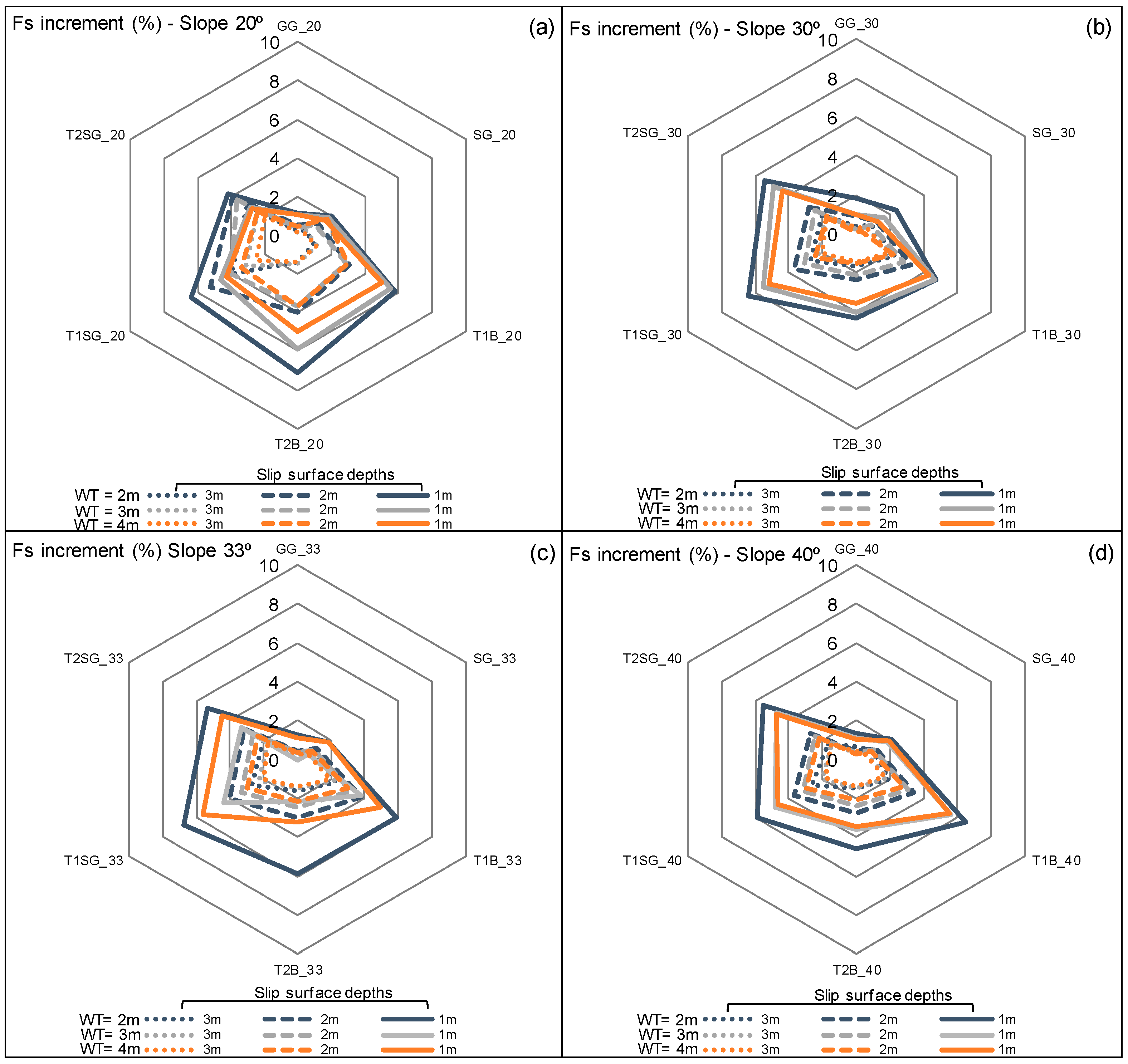
3.1. Mechanical Reinforcement of Combined Vegetation on Slope Stability

Figure 5 shows the FS increment (%) for the vegetation combinations considered and for each of the slope inclinations selected. For all of them, the maximum FS increment registered was less than 8%, with the lowest value for the deepest slip surface of less than 1%. An interesting finding is that as the water table distance to the surface decreases (i.e., the water table rises), the higher the effect of vegetation on the FS. Regardless of the slope inclination, the FS increment for the same vegetation combination is the highest for a WT = 2 m compared to the ones for WT of 3 m or 4 m. This means that as the water table rises, the overall stability is reduced, but the positive effect of vegetation increases.
With regard to failure surfaces, the vegetation effects for all types of slope inclination are observed mostly at the shallowest slip surface (1 m), and this is justified by the fact that the maximum rooting depth for all vegetation types was 1 m. In fact, for a rotational surface, only the initial part and the final part of the slip surface intercept the rooted zone.
With regard to the vegetation covering, a slope covered by only grass or by both shrubs and grass can only improve the FS by maximum about 2%, while a slope covered by trees can improve the FS by more than 6%.
The best combinations for all slopes are those including trees (T1B, T2B, T1SG, and T2SG), with a tendency to give higher FS increment in the combinations T1SG and T2SG, due to the entire vegetation coverage. This indicates that as expected, the highest mechanical reinforcement is given by the trees due to the highest additional root cohesion to the soil, but the best combination is the one including also shrubs and grasses along the slope, meaning the highest coverage of the slope by vegetation.
When comparing the series including trees, it is possible to observe that the higher FS increment is given by the combination with T1 (Norway spruce). By looking at the rooting depth and the additional root cohesion of the two different tree species (Table 4), it seems of higher importance to have a deeper root system with a lower additional cohesion (T1), instead of having a shallower root system with higher additional cohesion (T2).

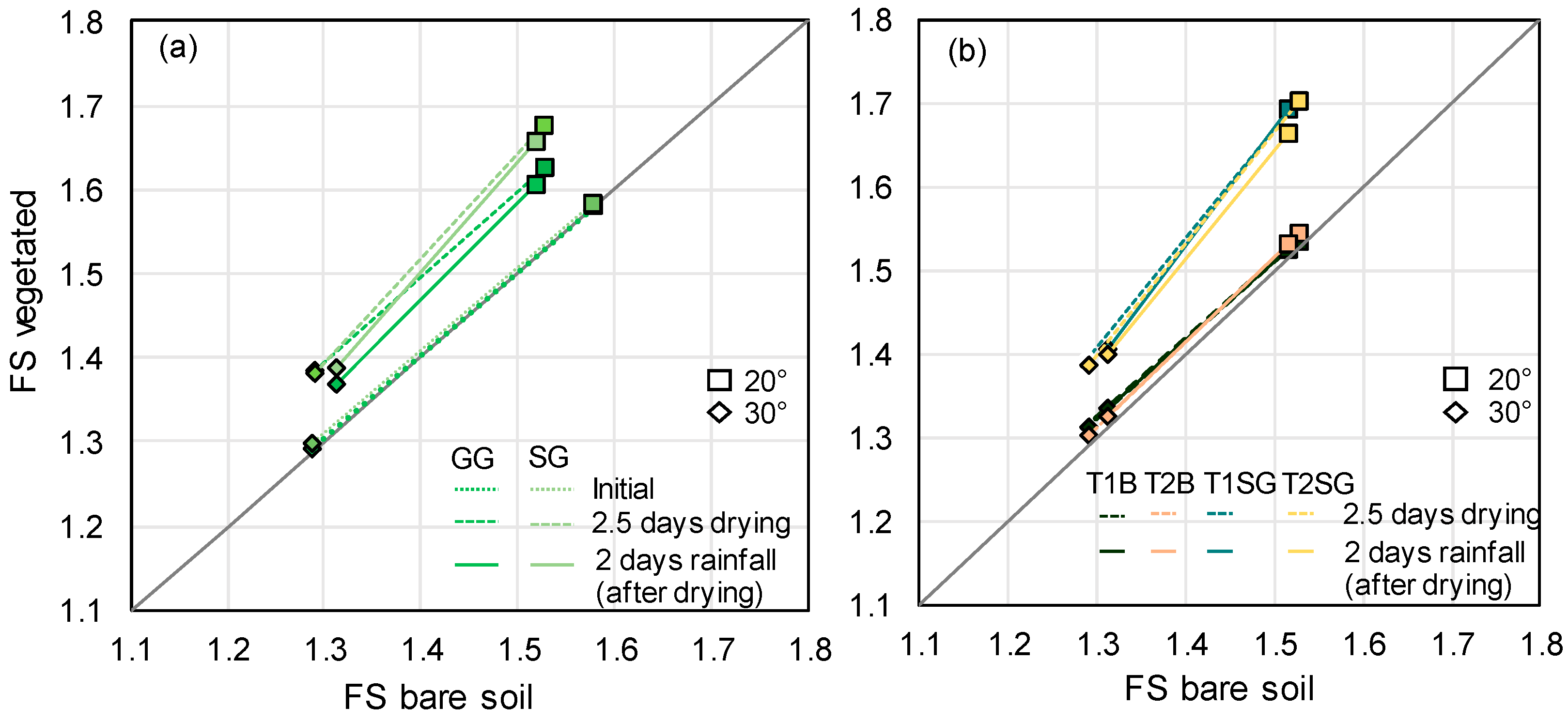
3.2. Hydro-Mechanical Reinforcement of Combined Vegetation

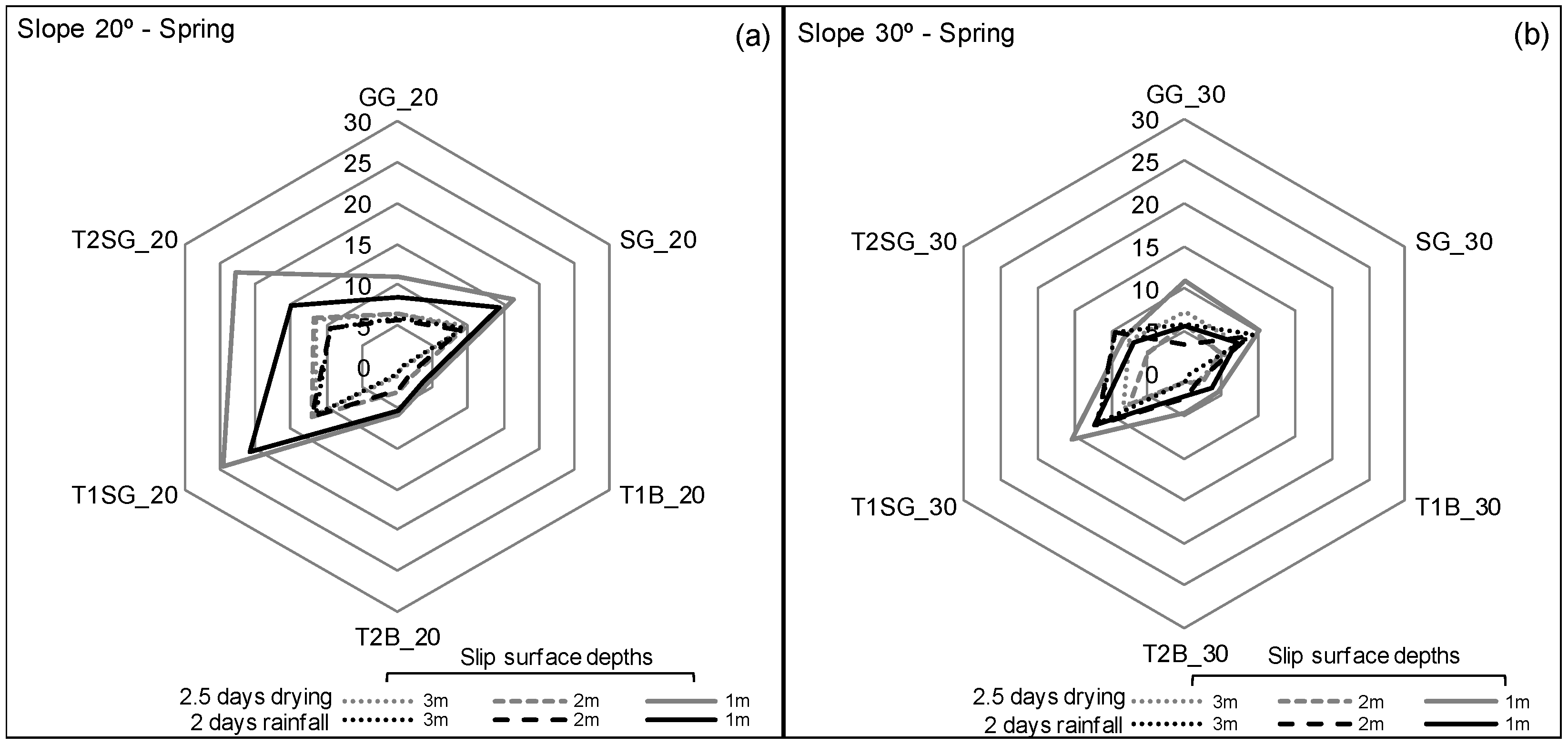
3.2.1. Spring Season—May

The coupled hydrological and mechanical reinforcement from the vegetation on slope stability needs to be studied in close relation with the season of the year. The methodology in Figure 2 for this case was adopted including also the hydrometeorological analysis as input for the hydrological modeling, which in turn represents the input to the slope stability modeling.
Figure 6 shows the increment of FS (%) obtained for the different vegetation combinations respectively after 2.5 days of drying (left graph), and at the end of 2 days of rainfall, for the three slip surface depths considered. The simulations were done only for the slope of 20° (Figure 6a) and 30° (Figure 6b) and for an initial water table of 3 m depth, which represent typical inclinations and water table position for ravines found in Norway.
For the slope of 20° inclination, the FS increment registered at the shallowest surface (1 m) increases from a maximum of about 6%, only considering the mechanical reinforcement (Figure 5a), up to a maximum of about 25%, when including the hydrological reinforcement due to drying (gray line in Figure 6a). On the other hand, for the most critical surface among the three analyzed (3 m depth), the FS increment changes from a maximum of about 4% to a maximum value ranging between 5% and 10%.
Likewise, for the slope of 30° inclination, the FS increment registered at the shallowest surface (1 m) increases from a maximum of about 5%, only considering the mechanical reinforcement (Figure 5b), up to a maximum of about 15%, when including the hydrological reinforcement due to drying (gray line in Figure 6b). For the most critical surface (3 m depth), the FS increment changes from a maximum of about 2% up to a maximum value of about 5%.
This indicates that even though the mechanical reinforcement has very little effect outside the rooted zone, there is continued improvement due to the hydrological activities of the roots, mostly by up taking of water and changing the pore pressure regime due to the evapotranspiration process.
When rainfall occurs, the FS is reduced due to water infiltration into the soil, increasing the pore water pressure. Having vegetation present in the slope influences the hydraulic properties of the soil permeated by roots, so during modeling, it could be considered to introduce a change of hydraulic conductivity of the vegetated soil, as suggested in Figure 3. However, for simplicity and due to lack of data (no lab tests were conducted), in this study, the hydraulic properties were assumed to be unchanged between the bare and vegetated soil. This is assumed to be conservative for the case where vegetation has shown to reduce the permeability of the soil and thus the water infiltration rate, or alternatively optimistic where the vegetation has shown to increase the soil permeability.
In this study, results from a simulated rainfall event of 2 days in the spring season show that the FS increment is slightly reduced compared to following the drying event, as expected, for both the slopes of 20° and 30° of inclination (Figure 6a,b black lines). However, when comparing these results to those obtained for the case “only mechanical reinforcement” (Figure 5a,c), the latter still have the lowest FS increment recorded. This is due to the difference in initial pore water regime because of the antecedent drying period, which unequivocally has modified the hydrological conditions due to the vegetation activity.
In general, from the shape of the radar graphs, it is possible to observe that the best combinations were those including shrubs and grass, specifically SG, T1SG, and T2SG.
For comparison purposes, Figure 6 shows the FS obtained for the spring season grouped in two main graphs: one related to low height vegetation—only grasses, or shrubs and grasses (Figure 7a)—and another one that considers either only high vegetation or mixed high vegetation and low height vegetation (Figure 7b). The FS vegetated vs. the FS bare trends are shown for the slope inclinations of 20° and 30°, and for the deepest slip surface (3 m), which can be considered as the lower bound of the expected FS increment due to vegetation. From these graphs, it is possible to observe, on the basis of the FS for a bare slope, what to expect for a vegetated combination in a typical spring situation:
  • After 2.5 days of drying;
  • After 2 days of rainfall (2 mm/d)—after the slope has been exposed to 2.5 days of drying.
As expected, the FS values calculated for a 20° slope are higher than the ones calculated for a deeper inclination of the slope (30°).
Most of the trend lines have a slope almost parallel to the bisector line and a certain intercept, except for the cases T1B and T2B, where the trend lines are almost overlapping the bisector line (Figure 7b). This means that for any FS registered in a bare slope, regardless of the slope inclination, there is an almost equal value of FS for the combination with only trees on the top and bare soil along the slopes (T1B and T2B); i.e., there is no improvement in FS by the addition of trees to the top of the slope. This is also shown in Figure 5, where the combinations including only trees have shown to always give the lowest FS increment. This could be attributed to the non-complete covering of the slope by vegetation, for the case including only trees at the top of the slope (Figure 4). The combinations T1B and T2B are the only two combinations that do not have vegetation coverage also along the slope (Table 3).
It can be stated that to be effective in reinforcing a river/stream embankment from a hydro-mechanical point of view, the vegetation should cover the entire slope (both the top part and the slope).

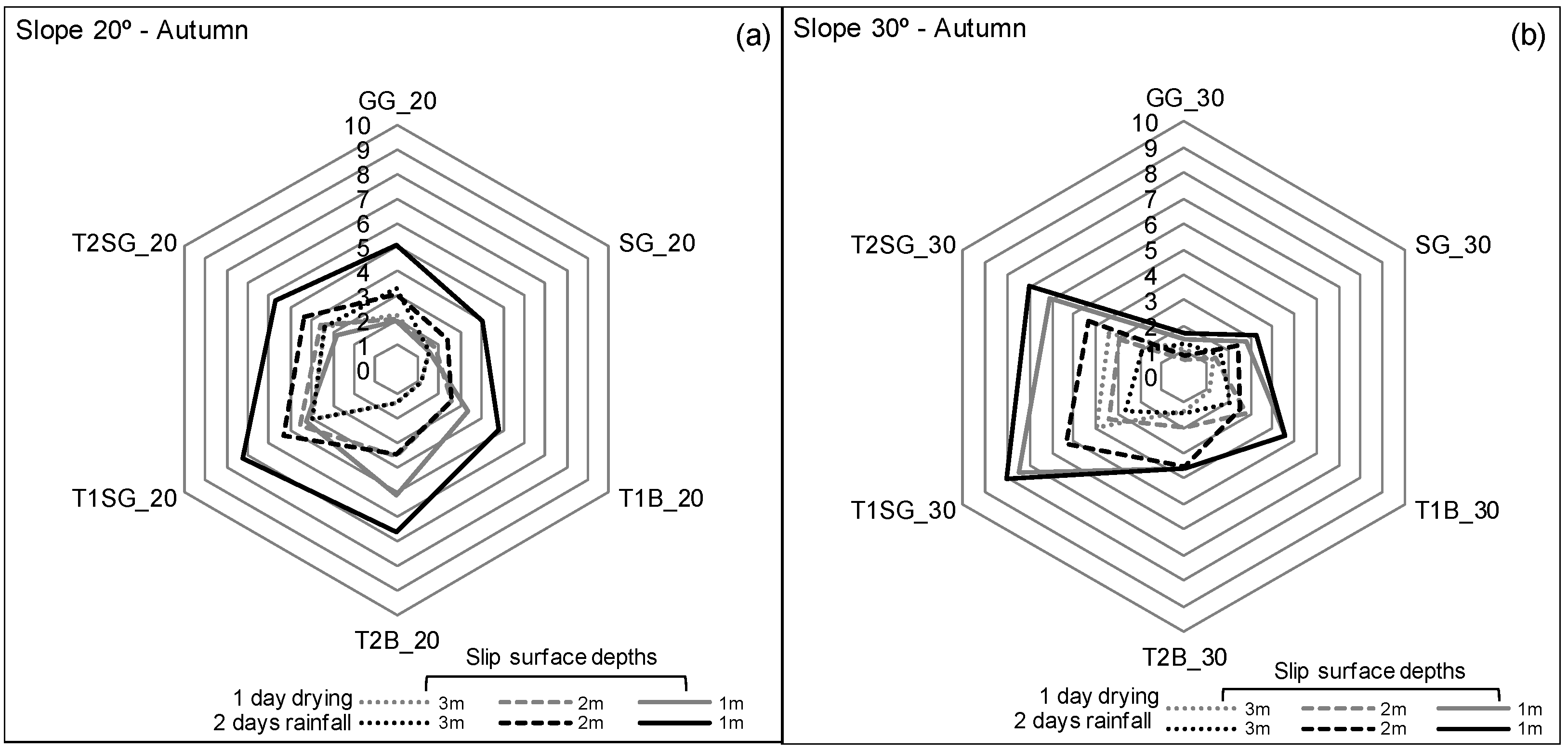
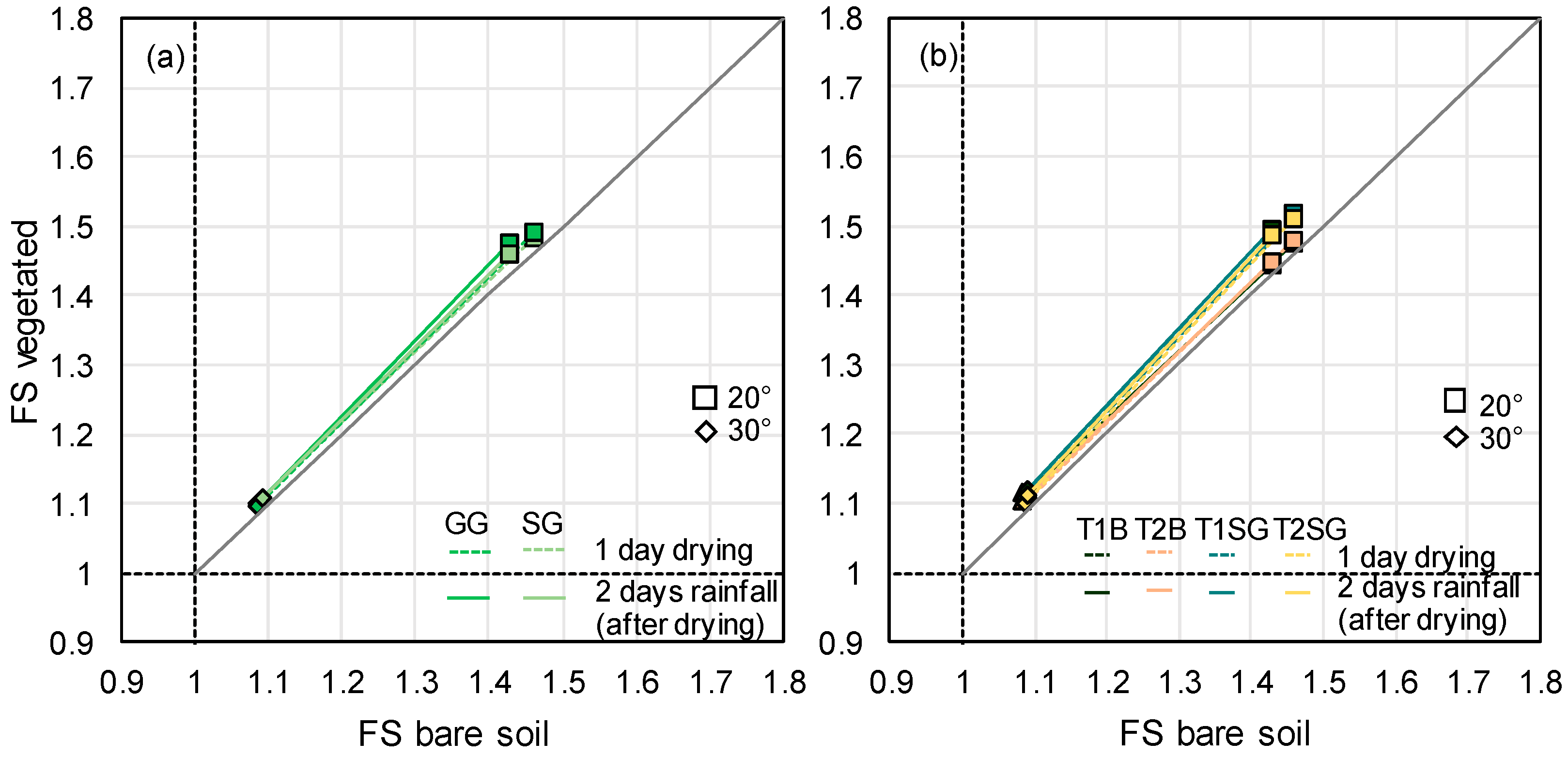
3.2.2. Fall Season—October

The same evaluations performed for the spring season were also carried out for the fall season, with the only exception that a soil cover fraction of 70% of the vegetated slopes was considered as a plausible reduction of the plant coverage during this season.
Figure 8 shows the FS increment evaluated for the same slope inclinations considering 1 day of drying, followed by 2 days of rainfall respectively for a 20° (Figure 8a) and 30° (Figure 8b) slope inclination.
The FS increment varied between a minimum of 1% for the deepest shear surface and a maximum of 8% for the shallowest shear surface in both slopes.
When compared to the case where only mechanical reinforcement is considered (Figure 5b), the difference in FS increment is not as remarkable as it was for the spring case, but it is relatively similar. This means that in the autumn season, the hydrological reinforcement is not as high as during the spring season. It is also interesting to notice that for all the slip surface depths, the FS increment due to vegetation was higher after the rainfall (black lines in Figure 8) compared to the case after drying (gray lines). This means that as the situation is worsened due to rainfall infiltration, the absolute FS values decrease, but the relative values of FS increment become higher (i.e., the FS was worsened more significantly in the bare soil scenario after rainfall than in the vegetated scenarios). In the spring season, the FS increment was higher after drying than after rainfall, whereas in the fall season, the FS increment was higher after rainfall. This shows that vegetated slopes have higher influence following rainfall in the wet season than in the dry season, despite an overall lower FS increment.
Figure 9 shows the FS vegetated vs. FS bare trends for both the low height vegetation and the mixed high and low height vegetation
From these graphs, it is possible to observe, based on the FS for a bare slope, what to expect for a vegetated combination in a typical autumn situation:
  • After 1 day of drying;
  • After 2 days of rainfall (3.2 mm/d)—after the slope has been exposed to 1 day of drying.
Here, the trend lines for all vegetation combinations have a very small intercept. In addition, contrary to the spring season, the contribution given by the trees only scenario does not differ much from the other vegetation combinations that cover the entire slope. Combinations including trees appear to contribute more to the slope stability compared to low height vegetation.
However, the hydro-mechanical reinforcement of vegetation in fall season seems to be not as important as in the spring season.

4. Discussion

The study described in this paper investigates the effect of different combinations of vegetation species on the stability reinforcement of streambanks. The main point for discussions from the analyses of benchmark cases are as follows:
  • By only considering the mechanical reinforcement, the increase of FS due to the presence of roots does not exceed 8%.
The mechanical effect of roots is exerted within the rooting zone (i.e., the area of soil permeated by roots), as the root-permeated material behaves as a composite material in which the stresses are distributed between the solid skeleton and the root network. In this case, since the maximum depth of roots was 1 m, the critical shear surface was below the rooting depth in most cases, and this explained why by only considering a mechanical reinforcement through additional root cohesion, the FS increment was negligible.
  • To be effective in reinforcing a river/stream embankment from a hydro-mechanical point of view, the vegetation should cover the entire slope (both the top part and the slope).
This is expected, since vegetation along streambanks finds maximum effectiveness when it completely covers soil. This is not only to improve slope stability but also to reduce other possible negative factors that might affect the slope overall stability such as erosion both along the slope and at the toe of the slope [20,52].
  • In the spring season, for a typical southeastern Norwegian catchment, the increase of FS due to vegetation reaches values up to 20% for the shallowest slip surface (1 m deep) and a maximum of 10% for the deepest shear surface (3 m deep), showing that hydrological reinforcement of the vegetation is more pronounced in the spring season compared to the fall season, where the FS increment due to the vegetation cover is maximum 8%. This is also expected, since plant activity varies seasonally depending on its physiological requirement [53]. Similar studies in different climate conditions [54,55] have confirmed that vegetation exerts its maximum effect in terms of hydrological reinforcement during the dry seasons, confirming that the plant–water uptake is the main hydrological mechanism contributing to slope stability.
  • Low-height vegetation has shown to be a good hydrological reinforcement in spring season, while the mixed combination including trees gives the highest mechanical reinforcement.
  • This study demonstrates that a combination of vegetation, trees–shrubs–grasses, gives the highest reinforcement, indicating this would be the best solution in terms of slope stability and expected biodiversity enhancement along riverbanks with soil and slope properties such as the one studied in this paper.
  • In the spring season, the FS increment after rainfall is less than after drying, whereas in the autumn season, the FS increment after rainfall is higher than after drying. Although the overall FS for autumn is lower, the vegetation is shown to have a more stabilizing effect following a rainfall than in the spring season; i.e., the FS for the bare slope was reduced more compared with the vegetated slopes in the spring than in the autumn.
The results above are only valid for the types of ravines with input parameters similar to those used in this study. The simulations in this study were conducted by using benchmark cases and data taken from the literature, only considering one type of soil and with all the limitations associated with this type of analyses (i.e., ideal slope geometry, root/shoot features from different environmental contexts, etc.).

5. Conclusions and Further Works

In this study, a methodological approach to assess the hydro-mechanical reinforcement of vegetation on slope stability was proposed and adopted. The methodology includes the required steps for the evaluation of slope stability by including the multiple effects that vegetation can provide to soil properties and soil–atmospheric interaction. All the factors that could be changed by the presence of vegetation were classified and referred to current available scientific literature, highlighting the knowledge gaps still remaining. Then, the approach was applied to benchmark cases of a Norwegian ravine, considering different slope inclinations and initial water tables. The analyses were carried out for two cases: (1) only considering the mechanical reinforcement of vegetation and (2) considering a coupled hydrological and mechanical reinforcement of vegetation. The results showed that the purely mechanical contribution of vegetation to slope stability could not be decoupled from the hydrological reinforcement, since in all cases, the critical shear surface occurred partly outside the rooted zone. Very few attempts so far have been done to evaluate the effects of vegetation on the stability of streambanks in Norway [10], and this is only a small contribution to this topic. Further studies are needed to assess whether vegetation can be a viable solution for improving slope stability of riverbanks and streambanks in Nordic regions. The novel open source tool Plant-Best [56], which detects also landslide prone zone in a GIS environment, could be used for a Norwegian stream context and provide a validation of the work carried out in this study.
Furthermore, additional simulations must include extreme rainfall intensities and climate change projections to evaluate the vegetation effects on stability of streambanks in a changing climate.
Possible future activities that would improve the use of vegetation as NBS along streambanks in Norway in a quantifiable manner are the following:
  • Investigations of real bank failures observed in Norwegian ravines (i.e., type of soil involved, vegetation, slopes, meteorological data, etc.);
  • Investigation on the root/shoot features (i.e., root depths, root additional cohesion, root structure, tree height, tree density, vegetation combination) in a real case study site of a Norwegian catchment, also looking at other vegetation species;
  • Application of the methodological approach in Figure 2, including the additional effects of roots on slope stability modeling (i.e., change in soil permeability, soil porosity);
  • Modeling of the effects of seasonal weather patterns and climate change on slope stability.

Author Contributions

Conceptualization, V.C., K.R., B.K., C.E., and Ø.H.; methodology, V.C.; analyses, V.C., K.R. and Anniken Helene Aalerud; writing—original draft preparation, V.C.; writing—review and editing, C.E. and K.R.; supervision, B.K. and Ø.H.; project administration, V.C. All authors have read and agreed to the published version of the manuscript.

Funding

This research received no external funding.

Institutional Review Board Statement

Not applicable.

Informed Consent Statement

Not applicable.

Data Availability Statement

Not applicable.

Conflicts of Interest

The authors declare no conflict of interest.

References

  1. Brondizio, E.S.; Settele, J.; Díaz, S.; Ngo, H.T. Global Assessment Report on Biodiversity and Ecosystem Services of the Intergovernmental Science-Policy Platform on Biodiversity and Ecosystem Services; IPBES Secretariat: Bonn, Germany, 2019. [Google Scholar]
  2. Hanssen-Bauer, I.; Førland, E.J.; Haddeland, I.; Hisdal, H.; Mayer, S.; Nesje, A.; Nilsen, J.E.Ø.; Sandven, S.; Sandø, A.B.; Sorteberg, A.; et al. Klima i Norge 2100 Kunnskapsgrunnlag for Klimatilpasning, Oppdatert i 2015; Norsk klimaservicesenter: Oslo, Norway, 2015. [Google Scholar]
  3. Hubble, T.C.T.; Docker, B.B.; Rutherfurd, I.D. The role of riparian trees in maintaining riverbank stability: A review of Australian experience and practice. Ecol. Eng. 2010, 36, 292–304. [Google Scholar] [CrossRef]
  4. Lundekvam, H.E.; Romstad, E.; Øygarden, L. Agricultural policies in Norway and effects on soil erosion. Environ. Sci. Policy 2003, 6, 57–67. [Google Scholar] [CrossRef]
  5. Simon, A.; Collison, A.J. Quantifying the mechanical and hydrologic effects of riparian vegetation on streambank stability. Earth Surf. Process. Landf. 2002, 27, 527–546. [Google Scholar] [CrossRef]
  6. Gonzalez-Ollauri, A.; Stokes, A.; Mickovski, S.B. A novel framework to study the effect of tree architectural traits on stemflow yield and its consequences for soil-water dynamics. J. Hydrol. 2020, 582, 124448. [Google Scholar] [CrossRef]
  7. Ng, C.W.W.; Leung, A.K.; Woon, K.X. Effects of soil density on grass-induced suction distributions in compacted soil subjected to rainfall. Can. Geotech. J. 2013, 51, 311–321. [Google Scholar] [CrossRef]
  8. Garg, A.; Coo, J.L.; Ng, C.W.W. Field study on influence of root characteristics on soil suction distribution in slopes vegetated with Cynodon dactylon and Schefflera heptaphylla. Earth Surf Process Landf. 2015, 40, 1631–1643. [Google Scholar] [CrossRef]
  9. Ng, C.W.W.; Garg, A.; Leung, A.K.; Hau, B.C.H. Relationships between leaf and root area indices and soil suction induced during drying–wetting cycles. Ecol. Eng. 2016, 91, 113–118. [Google Scholar] [CrossRef] [Green Version]
  10. Pollen-Bankhead, N.; Simon, A. Hydrologic and hydraulic effects of riparian root networks on streambank stability: Is mechanical root-reinforcement the whole story? Geomorphology 2010, 116, 353–362. [Google Scholar] [CrossRef]
  11. Gonzalez-Ollauri, A.; Mickovski, S.B. Plant-soil reinforcement response under different soil hydrological regimes. Geoderma 2017, 285, 141–150. [Google Scholar] [CrossRef] [Green Version]
  12. Dias, A.S.; Pirone, M.; Urciuoli, G. Review on the methods for evaluation of root reinforcement in shallow landslides. In Proceedings of the World Landslide Forum, Ljubljana, Slovenia, 30 May–2 June 2017; Springer: Cham, Switzerland, 2017; pp. 641–648. [Google Scholar]
  13. Foresta, V.; Capobianco, V.; Cascini, L. Influence of grass roots on shear strength of pyroclastic soils. Can. Geotech. J. 2020, 57, 1320–1334. [Google Scholar] [CrossRef] [Green Version]
  14. Cardile, G.; Pisano, M.; Moraci, N.; Ricciardi, A. Reliability analysis of root-reinforced slopes. In Proceedings of the XVII ECSMGE-2019, Reykjavik, Iceland, 1–6 September 2019. [Google Scholar]
  15. Pollen, N.; Simon, A. Estimating the mechanical effects of riparian vegetation on stream bank stability using a fiber bundle model. Water Resour. Res. 2005, 41. [Google Scholar] [CrossRef]
  16. Arnone, E.; Caracciolo, D.; Noto, L.V.; Preti, F.; Bras, R.L. Modeling the hydrological and mechanical effect of roots on shallow landslides. Water Resour. Res. 2016, 52, 8590–8612. [Google Scholar] [CrossRef]
  17. Kottek, M.; Grieser, J.; Beck, C.; Rudolf, B.; Rubel, F. World Map of the Köppen-Geiger Climate Classification Updated; Gebrüder Borntraeger: Berlin, Germany, 2006. [Google Scholar]
  18. Firvold, L.H. Trær Som Stabiliserende Element i Leirskråninger—Med Spesiell Relevans til Romerike; lnstitutt for skogfag Norges landbrukshøgskole: Oslo, Norway, 1991. (In Norwegian) [Google Scholar]
  19. Krzeminska, D.; Kerkhof, T.; Skaalsveen, K.; Stolte, J. Effect of riparian vegetation on stream bank stability in small agricultural catchments. Catena 2019, 172, 87–96. [Google Scholar] [CrossRef]
  20. Bordoloi, S.; Ng, C.W.W. The effects of vegetation traits and their stability functions in bio-engineered slopes: A perspective review. Eng. Geol. 2020, 257, 105742. [Google Scholar] [CrossRef]
  21. Ni, J.J.; Leung, A.K.; Ng, C.W.W.; Shao, W. Modelling hydro-mechanical reinforcements of plants to slope stability. Comput. Geotech. 2018, 95, 99–109. [Google Scholar] [CrossRef]
  22. Capobianco, V.; Cascini, L.; Cuomo, S.; Foresta, V. Wetting-Drying Response of an Unsaturated Pyroclastic Soil Vegetated with Long-Root Grass. Environ. Geotech. 2020, 1–18. [Google Scholar] [CrossRef]
  23. Preti, F.; Dani, A.; Laio, F. Root profile assessment by means of hydrological, pedological and above-ground vegetation information for bio-engineering purposes. Ecol. Eng. 2010, 36, 305–316. [Google Scholar] [CrossRef]
  24. Huang, M.; Barbour, S.L.; Carey, S.K. The impact of reclamation cover depth on the performance of reclaimed shale overburden at an oil sands mine in Northern Alberta, Canada. Hydrol. Process. 2015, 29, 2840–2854. [Google Scholar] [CrossRef]
  25. Allen, R.G.; Pereira, L.S.; Raes, D.; Smith, M. Crop Evapotranspiration—Guidelines for Computing Crop Water Requirements; FAO Irrigation and Drainage Paper 56; Food and Agriculture Organization of the United Nations: Rome, Italy, 1998. [Google Scholar]
  26. Mathurn, S.; Rao, S. Modeling water uptake by plant roots. J. Irrig. Drain. Eng. 1999, 125, 159–165. [Google Scholar] [CrossRef]
  27. Feddes, R.A.; Kowalik, P.; Malinka, K.K.; Zaradny, H. Simulation of field water uptake by plants using a soil water dependent root extraction function. J. Hydrol. 1976, 31, 13–26. [Google Scholar] [CrossRef]
  28. Feddes, R.A.; Hoff, H.; Bruen, M.; Dawson, T.; De Rosnay, P.; Dirmeyer, P.; Jackson, R.B.; Kabat, P.; Kleidon, A.; Lilly, A.; et al. Modeling root-water uptake in hydrological and climate models. Bull. Am. Meteorol. Soc. 2001, 82, 2797–2809. [Google Scholar] [CrossRef] [Green Version]
  29. Prasad, R. A linear root water uptake model. J. Hydrol. 1988, 99, 297–306. [Google Scholar] [CrossRef]
  30. Wynn, T.M.; Mostaghimi, S.; Burger, J.A.; Harpold, A.A.; Henderson, M.B.; Henry, L.A. Variation in root density along stream banks. J. Environ. Qual. 2004, 33, 2030–2039. [Google Scholar] [CrossRef] [PubMed]
  31. Kalliokoski, T. Root System Traits of Norway Spruce, Scots Pine, and Silver Birch in Mixed Boreal Forests: An Analysis of Root Architecture, Morphology, and Anatomy. Ph.D Thesis, Helsingin yliopisto, Helsinki, Finland, 2011. [Google Scholar]
  32. GEO-SLOPE International Ltd. Seepage Modeling with SEEP/W. 2012. Available online: http://downloads.geo-slope.com/geostudioresources/8/0/6/books/seep%20modeling.pdf?v=8.0.7.6129 (accessed on 29 March 2020).
  33. Bishop, A.W. The use of the slip circle in the stability analysis of slopes. Geotechnique 1955, 5, 7–17. [Google Scholar] [CrossRef]
  34. Chirico, G.B.; Borga, M.; Tarolli, P.; Rigon, R.; Preti, F. Role of vegetation on slope stability under transient unsaturated conditions. Procedia Environ. Sci. 2013, 19, 932–941. [Google Scholar] [CrossRef]
  35. Preti, F. Forest protection and protection forest: Tree root degradation over hydrological shallow landslides triggering. Ecol. Eng. 2013, 61, 633–645. [Google Scholar] [CrossRef]
  36. Simon, A.; Curini, A.; Darby, S.E.; Langendoen, E.J. Streambank mechanics and the role of bank and near-bank processes in incised channels. In Incised River Channels: Processes, Forms, Engineering, and Management; Darby, S.E., Simon, A., Eds.; John Wiley & Sons: London, UK, 1999; pp. 123–152. [Google Scholar]
  37. Pollen-Bankhead, N.; Simon, A. Enhanced application of root-reinforcement algorithms for bank-stability modeling. Earth Surf. Process. Landf. 2009, 34, 471–480. [Google Scholar] [CrossRef]
  38. Bischetti, G.B.; Chiaradia, E.A.; Simonato, T.; Speziali, B.; Vitali, B.; Vullo, P.; Zocco, A. Root strength and root area ratio of forest species in Lombardy (Northern Italy). In Eco-and Ground Bio-Engineering: The Use of Vegetation to Improve Slope Stability; Springer: Dordrecht, The Netherlands, 2007; pp. 31–41. [Google Scholar] [CrossRef]
  39. Schmid, I.; Kazda, M. Vertical distribution and radial growth of coarse roots in pure and mixed stands of Fagus sylvatica and Picea abies. Can. J. For. Res. 2001, 31, 539–548. [Google Scholar] [CrossRef]
  40. Hales, T.C.; Miniat, C.F. Soil moisture causes dynamic adjustments to root reinforcement that reduce slope stability. Earth Surf. Process. Landf. 2017, 42, 803–813. [Google Scholar] [CrossRef] [Green Version]
  41. Mauer, O.; Palátová, E. The role of root system in silver birch (Betula pendula Roth) dieback in the air-polluted area of Krušné hory Mts. J. Sci. 2003, 49, 191–199. [Google Scholar] [CrossRef] [Green Version]
  42. Leung, A.K.; Boldrin, D.; Liang, T.; Wu, Z.Y.; Kamchoom, V.; Bengough, A.G. Plant age effects on soil infiltration rate during early plant establishment. Géotechnique 2018, 68, 646–652. [Google Scholar] [CrossRef] [Green Version]
  43. Jotisankasa, A.; Sirirattanachat, T. Effects of grass roots on soil-water retention curve and permeability function. Can. Geotech. J. 2017, 54, 1612–1622. [Google Scholar] [CrossRef] [Green Version]
  44. Ghestem, M.; Sidle, R.C.; Stokes, A. The influence of plant root systems on subsurface flow: Implications for slope stability. Bioscience 2011, 61, 869–879. [Google Scholar] [CrossRef]
  45. Rahardjo, H.; Satyanaga, A.; Leong, E.C.; Santoso, V.A.; Ng, Y.S. Performance of an instrumented slope covered with shrubs and deeprooted grass. Soils Found. 2014, 54, 417–425. [Google Scholar] [CrossRef] [Green Version]
  46. Askarinejad, A. Failure Mechanisms in Unsaturated Silty Sand Slopes Triggered by Rainfall; vdf Hochschulverlag AG: ETH Zurich, Switzerland, 2015; Volume 248. [Google Scholar]
  47. Byrne, K.A.; Kiely, G.; Leahy, P. CO2 fluxes in adjacent new and permanent temperate grasslands. Agric. For. Meteorol. 2005, 135, 82–92. [Google Scholar] [CrossRef]
  48. Garg, A.; Leung, A.K.; Ng, C.W.W. Transpiration reduction and root distribution functions for a non-crop species Schefflera heptaphylla. Catena 2015, 135, 78–82. [Google Scholar] [CrossRef] [Green Version]
  49. Li, D.; Gu, X.; Pang, Y.; Chen, B.; Liu, L. Estimation of forest aboveground biomass and leaf area index based on digital aerial photograph data in Northeast China. Forests 2018, 9, 275. [Google Scholar] [CrossRef] [Green Version]
  50. Wang, T.; Tigerstedt, P.M.A.; Viherä-Aarnio, A. Photosynthesis and canopy characteristics in genetically defined families of silver birch (Betula pendula). Tree Physiol. 1995, 15, 665–671. [Google Scholar] [CrossRef]
  51. Cherubini, F.; Vezhapparambu, S.; Bogren, W.; Astrup, R.; Strømman, A.H. Spatial, seasonal, and topographical patterns of surface albedo in Norwegian forests and cropland. Int. J. Remote Sens. 2017, 38, 4565–4586. [Google Scholar] [CrossRef]
  52. Micheli, E.R.; Kirchner, J.W. Effects of wet meadow riparian vegetation on streambank erosion. 2. Measurements of vegetated bank strength and consequences for failure mechanics. Earth Surf. Process. Landf. 2002, 27, 687–697. [Google Scholar]
  53. Mancuso, S.; Viola, A. Brilliant Green: The Surprising History and Science of Plant Intelligence; Island Press: London, UK, 2015. [Google Scholar]
  54. Gonzalez-Ollauri, A.; Mickovski, S.B. Hydrological effect of vegetation against rainfall-induced landslides. J. Hydrol. 2017, 549, 374–387. [Google Scholar] [CrossRef] [Green Version]
  55. Comegna, L.; Damiano, E.; Greco, R.; Guida, A.; Olivares, L.; Picarelli, L. Effects of the vegetation on the hydrological behavior of a loose pyroclastic deposit. Procedia Environ. Sci. 2013, 19, 922–931. [Google Scholar] [CrossRef] [Green Version]
  56. Gonzalez-Ollauri, A.; Mickovski, S.B. Plant-Best: A novel plant selection tool for slope protection. Ecol. Eng. 2017, 106, 154–173. [Google Scholar] [CrossRef] [Green Version]
Figure 1. The area considered in the desk study. The catchment is located northeast of Oslo, and the study area is one of the tributary streams of the Glomma river. On the right side, the focus area with the surficial geology map; blue is marine sediments under the marine limit, and yellow is river and stream sediments consisting of river plains, terraces, and fans.
Sustainability 13 04046 g001
Figure 2. Example of streambanks in a Norwegian southeastern catchment: (a) highly vegetated with grass, shrubs, and trees and (b) barely vegetated.
Sustainability 13 04046 g002
Figure 3. Methodological approach for slope stability modeling including vegetation–soil parameters and processes influenced by the presence of vegetation (root density/architecture/depth and canopy area).
Sustainability 13 04046 g003
Figure 4. Benchmark bank showing the top and slope regions.
Sustainability 13 04046 g004
Figure 5. Factor of safety increment (%) calculated for the different cover combinations at (a) 20°, (b) 30°, (c) 33°, and (d) 40° of slope inclination. The ID of each vertex reflects the combinations proposed in Table 3, and the last two numbers correspond to the slope inclination (e.g., T1SG_20 is the combination including the tree Spruce (T1) at the top and shrubs and grass on the slope, for a 20° slope inclination). The radar graphs are made for three different slip surfaces respectively at 1, 2, and 3 m distance from the slope surface.
Sustainability 13 04046 g005
Figure 6. Factor of safety increment calculated for different vegetation combinations at (a) 20° and (b) 30° of slope inclination—spring season. The gray curves represent the factor of safety (FS) increment obtained after the drying, while the black curves are the result of 2 days of rainfall applied after the drying. The ID of each vertex reflects the combinations proposed in Table 3, and the last two numbers correspond to the slope inclination (e.g., T1SG_20 is the combination including the tree Spruce (T1) at the top and shrubs and grass on the slope, for a 20° slope inclination). The radar graphs are made for the same three different slip surfaces respectively at 1 m (continuous line), 2 m (dashed line), and 3 m (dotted line) of depth.
Sustainability 13 04046 g006
Figure 7. Factor of safety (FS) calculated for the different slope inclinations and vegetation combinations—spring season; (a) low height vegetation (only grass -GG, shrubs and grass—SG), (b) combinations including trees.
Sustainability 13 04046 g007
Figure 8. Factor of safety increment calculated for different vegetation combinations at (a) 20° and (b) 30° of slope inclination—autumn season. The gray lines represent the FS increment obtained after the drying, while the black lines are the result of 2 days of rainfall applied after the drying. The ID of each vertex reflects the combinations proposed in Table 3, and the last two numbers correspond to the slope inclination (e.g., T1SG_20 is the combination including the tree Spruce (T1) at the top and shrubs and grass on the slope, for a 20° slope inclination). The radar graphs are made for the same three different slip surfaces respectively at 1 m (continuous line), 2 m (dashed line), and 3 m (dotted line) of depth.
Sustainability 13 04046 g008
Figure 9. Factor of safety (FS) calculated for the different slope inclinations and vegetation combinations—fall season; (a) low height vegetation (only grass -GG, shrubs and grass—SG), (b) combinations including trees.
Sustainability 13 04046 g009
Table 1. Vegetation features and environmental conditions of the trees and shrubs studied.
TreesShrubs
Picea Abies
(Norway Spruce)
Betula Pubescens
(Downy Birch)
Salix Caprea
(Goat Willow)
Drainage and soil typeRoot depth is drainage dependentCan grow in soils with poor drainage Sandy/clay soil
Nutrients/minerals availabilityPrefer soils rich in nutrients -Calcareous soils
Soil depthDeep--
Humidity-Can grow in soils with high water contentDry/slightly moist
BiodiversityCan make the vegetative ground cover sparse with low biodiversitySeason dependent, but generally allows for rich biodiversity-
Coexistence with other speciesGrows deeper roots when mixed with other tree speciesGoodGood
Plant establishmentSlow at the beginning—poor for immediate stabilizationPioneer species, good for immediate stabilizationPioneer, especially good to repair landslide areas
Vegetative Propagation-Seeds and root shoots from the tree stumpShoots from tree stumps, branches and roots
RootsNormally flat with sinking roots. Deeper roots when growing with other tree speciesTap rootsDeep at first, then flat reaching out to the sides
Water consumption-High-
Treefall—Wind riskCan grow very tall—increased risk to wind damageNot specified—possibly no high treefall riskIt grows not taller than 10 m—no high treefall risk
Tree HeightHighHighCan be both tree and shrub
Table 2. Main soil properties of the soil studies and inclination of the benchmark slopes and water table conditions.
Slope and Soil ParametersValues
Slope height, H10 m
Inclination, I20°, 30°,33°, 40°
Unit weight, γ18.5 kN/m3
Cohesion, c′0 kPa
Friction angle, ϕ′33°
Initial water table, WT2 m, 3 m, 4 m
Table 3. Vegetation combinations and ID considered in the simulations.
Vegetation CombinationID
TopSlope
Bare soilBare soilB
GrassGrassGG
ShrubsGrassSG
Trees (Spruce)Bare soilT1B
Trees (Birch)Bare soilT2B
Trees (Spruce)Shrubs and grassT1SG
Trees (Birch)Shrubs and grassT2SG
Table 4. Values of average rooting depth (RD) and additional root cohesion (cr) for the vegetation species studied.
IDSpeciesRDReferencecrReference
m kPa
GMixed grasses0.6[30]0.35[19]
SSalix Caprea1.0[19]1.37[19]
T1Picea abies1.0[39]5.70[38]
T2Betula P.0.6[40,41] 7.18[19]
Table 5. Leaf Area Index (LAI) values used in the model for the vegetation species considered.
IDLAI (m2/m2)Reference
G1[47]
S2.5[48]
T14.4[49]
T23.0[50]
Table 6. Meteorological data used for the simulations in this study.
MonthAverage Temperature (°C)Average Relative HumidityAverage Wind Speed (m/s)Average Solar Radiation (J/Sec/m²)Average Albedo [51]
May100.726.155852.630.14
Oct4.750.904.361570.960.18
Publisher’s Note: MDPI stays neutral with regard to jurisdictional claims in published maps and institutional affiliations.

