Predicting Increase in Demand for Public Buses in University Students Daily Life Needs: Case Study Based on a City in Japan

Abstract

Accessibility and economic sustainability of public bus services (PBS) have been in a continuous decline in Japan’s countryside. Rural cities also suffer from population transformation toward industrial centers experiencing rapid economic growth. In the present study, we reviewed the current demand status of PBS in Kitami, a rural city in Japan that hosts a national university. The investigation was performed by examining students’ daily lives using a survey to collect data representing a portion of the population. The objective was to predict the change in demand rate for PBS concerning the necessities of everyday life from the perspective of university students as potential users of PBS. Intuitively, decision-makers at every level display a distinct prejudice toward alternatives that intend to change the long-lasting status quo, hence in the question sequence, a two-step verification probe was used to reveal a person’s actual perceived opinion. Accordingly, the respondents’ initial demand rate for PBS was around 60%; however, this score increased to 71% in the secondary confirmation. Afterward, using machine learning-based prediction methods, we could predict this demand at over 90% of F-measure, with the most reliable and stable prediction method reaching 80% by other daily life indicators’ weight. Finally, we supplied thorough evidence for our approach’s usability by collecting and processing the data’s right set regarding this study’s objective. This method’s highlighted outcomes would help to reduce the local governments’ and relevant initiatives’ adaptability time to demands and improve decision-making flexibility.

1. Introduction

Accessibility and economic sustainability of public bus services (PBS) have been in continuous decline in Japan’s countryside [1]. Moreover, rural cities suffer from population transition toward industrial centers due to rapid economic growth. Former studies concerning passenger transportation have generally discussed the definition of services, performance, management, private providers’ role, improved efficiency, pricing, and systematic travel user-demand supervision [2,3]. Modern studies regarding academic and industrial sectors focus on passenger satisfaction to encourage more public transportation by suggesting to provide advanced passenger transport systems based on individual’s preference of transportation [4,5].

In this context, it is essential to enhance the knowledge base in the passenger transportation field to provide a firm basis to empower policymakers with the ability to respond dynamically to ever-changing transportation needs. The majority of the data in the transportation field consists of official statistics created by the government or local authorities in Japan [6]. The data is usually collected by user surveys conducted in major cities or specific business sectors and often describes the reason for people’s movement, beginning and arrival points, and transportation means. Therefore, increasing the diversity of transportation statistics in Japan and discussing the challenges of each geographic region’s different needs and expectations to promote appropriate solutions have been the motivating factors to carry out this research.

Unlike large cities in Japan, the accessibility of PBS is limited in rural regions; consequently, transportation often depends on privately owned vehicles. While most rural Japanese residents prefer the comfort of owning a private car, worth noting is the importance of PBS for the elderly, students, non-permanent residents, and visitors.

Additionally, contemporary Japanese society faces many other issues; frequently highlighted points include a decrease in population, an aging society, and young people’s migration to metropolitan areas [7]. Beyond these, the increasing trend of ‘inward-looking orientation’ among young people urges researchers and managers to search for more psychological reasons behind the inward-looking orientation within the youth population [8]. While the government mentions social engagement as one of the essential factors contributing to the quality of student experience, most universities tend to focus more on the academic program rather than on cultural adjustment [9]. Nevertheless, those problems are eventually disrupting rural communities’ sustainability.

From a more global perspective, various regional studies have examined the influence of travel and tourism on the revitalization of rural regions suffering from various socio-economic deficiencies in developed and developing countries [10,11,12,13]. Particular studies have also concentrated on universities’ role in travel and tourism activities, especially the demand side of university students’ tourism consumption, to understand the university as an integrative part of society [14]. A study suggested that universities and host cities should acknowledge the potential contribution of university students to developing ecologically and socially sustainable communities [15]. Universities are also under increasing pressure to become more internationally oriented and provide their students a global experience related to the openness of their communities. From international students’ perspective, the desire to travel and the opportunity for fun or excitement are the primary motivators for undertaking an educational exchange, along with the host country’s climate, natural environment, hospitality, and tourist attractions [16]. Moreover, instead of isolating the campus areas, university students also want to be involved in their host cities’ social and cultural life [17].

In such a circumference, the scientific originality of this research evolves with identifying and presenting the straightforward points of daily life necessities that may expand the young population’s sustainability in the rural regions of Japan through findings from a case study. Considering that public transport services are one of the basic requirements of everyday life in a city, and observing that it does not serve effectively convinced us that it would be beneficial to conduct this study. We therefore strategically identified the entry point for this approach as inadequate PBS in a rural university town and its impact on the daily lives of university students. The proposed methodology offers a properly tested method to interpret the young individual opinions in this aspect. The discussed findings will help reduce adaptation time and improve decision-making flexibility for local governments and related enterprises in responding to students’ mobility demands. The objectives of this research were:

(1)

“To determine the impact of daily life needs that will significantly increase university students’ demand for PBS as potential users in a rural city.”

(2)

“To confirm the hypothesis that if an improvement occurs in PBS based on determined user needs, the demand on the user side will increase.”

(3)

“To offer a simple inferential statistics-based modeling that predicts how much the demand rate will increase on the user side if there is an improvement in PBS.”

Therefore, after examining the universities’ and students’ role in contributing to their host cities’ economy and recognizing the perception of this contribution to sustainable communities, we analyzed the “Student daily life after school hours” survey data conducted in 2019 at Kitami, Hokkaido.

Kitami (Figure 1) is the largest city in the Okhotsk subprefecture located in Japan’s northern part. The population of the city is around one hundred thousand residents and sparsely distributed among its boroughs. It hosts a national university, Kitami Institute of Technology, and a private college of nursing.

The Sea of Okhotsk is about 40–45 km north of the city. The sea’s polar nature causes an internationally well-known natural drift of ices that can be observed off the seacoast during the winter season. The city also has a famous association with winter sport, particularly curling.

Additionally, agriculture is one of the leading industries in the region, and Kitami is Japan’s largest producer of onions. The distance between Sapporo (the largest city of Hokkaido) and Kitami is around 300 km. Both bus and train services are operating daily; however, reservation in advance is required. Memanbetsu Airport serves the city located approximately 20 km from Kitami.

Intuitively, decision-makers at every level display a distinct prejudice toward alternatives that intend to change the long-lasting status quo [18]. Hence in the question sequence, a two-step verification probe was used to avoid this trap and reveal a person’s actual perceived opinion. The respondent’s initial demand rate for current PBS scored around 60% in favor; however, this score increased to 71% in the second confirmation. Next, four different machine learning-based prediction algorithms were tested with the user preference data collected in the survey applied as the feature set, which resulted in a reliable prediction of user preference change of over 90% for F-measure concerning real-life circumstances. Finally, we supplied thorough evidence for the usability of our approach in regional development decision-makers’ detailed data analyses. The study was also aimed to provide an entry-level micro-analysis, particularly for urban mobility studies when the secondary data is not yet achievable or limited.

The organization of the remaining sections is as follows. Section 2 overviews the literature. Section 3 and Section 4 present the proposed methodology and case study. Finally, Section 5 summarizes our research conclusions.

2. Literature Review

2.1. Situation Overview in Japan

A public transport system is expected to have two simultaneous objectives: to serve the public benefit and be profitable [19]. Still, these two goals do not go hand in hand according to each country’s particular circumstances. Public transport policy differs distinctly among the countries’ social structure and may focus on either the public benefit or the profitability. In Japan, profit-driven, privately owned, and publicly traded mass transit companies predominantly operate public transit systems [20].

Traditionally, Japanese regional passenger transportation systems evolved on railway subsidiaries until World War II [21]. However, after the war, during the rapid economic and industrial growth, unlike many other countries, the railway-based transport market’s condition shifted to private automobiles starting in the late ’60s. The new circumstance has triggered the abandonment of local railway lines by passengers, and disused lines were soon beginning to close due to unprofitability [22].

As a result of rapid economic growth, many households’ incomes became sufficient to afford more than one car in the late 1980s. The increasing trend for using private vehicles also caused a reduction in the passenger volume on public buses [23]. Many local bus companies began to experience financial difficulties, gradually resulting in the sudden abolition of PBS for local citizens even without a substitute [24]. In general, if passenger density is lower than five persons per inner-city bus line, the line is considered not profitable to maintain.

In Japan, as explained above, public transportation has been usually a service provided by private initiatives; simultaneously, especially in rural areas, people prefer private cars. In reality, there is not enough passenger demand for the profitability of public transport services provided by private companies. PBS can therefore never be an independent transportation alternative in rural Japan. Despite this fact, Japanese government policy has adopted the principle of self-sufficiency for public transportation [19].

Private companies in the countryside today offer many essential services required to maintain lifestyles in these regions, such as public transportation, logistics, and retail. However, these service providers are experiencing financial difficulties that cause them to withdraw from these markets because of declining demand and lack of the work power to carry out services, and weak long-term profitability expectations [25].

A new urban design and city planning concept called “compact city” has meanwhile been developed by government agencies to address the problems of aging and depopulated societies in rural areas according to people’s needs [26].

In parallel with the compact city concept, information and communication technologies (ICT) have emerged as active agents in stimulating people’s lives in rural communities [27,28,29,30]. Content analysis studies have shown that travel, tourism, and hospitality industries use ICT in various functional units and for different applications [31]. The functional unit for the ICT environmental impact assessment is generally defined as the change (quantification of improvement) triggered by a new ICT introduction [32]. Still, tourism informatics studies in Japan primarily focus on the informatics’ abilities to improve customer experiences regardless of promoting the tourist arrival to the tourism establishment [33].

On the other hand, the travel and tourism revenues’ contribution to the Japanese economy is small compared to the massive industrial sector’s income [34]. This performance depends on domestic travel and tourism spending that shapes the Japanese tourism industry’s unique economic characteristics. For example, domestic travel spending accounted for 91.8% of direct total travel and tourism expenditures (2.4% of total Japan GDP) in 2014 and 81% (7% of total Japan GDP) in 2019 [35,36]. The increased international spending share from 8.2% to 19% in the total tourism expenditures has relied on government agencies’ success in the last five years. Japan has moved up from ninth to fourth position on the travel and tourism competitiveness index among 140 countries. Inbound tourist arrivals have also increased from 20 million to 31 million all over Japan in the same period [37,38,39].

In the meantime, findings suggest that Japan’s inbound tourists’ increased rate is strongly dependent on the Asian market. The number and percentage of growth of sightseeing tourists are higher than those of other types. China has become the most significant source of inbound tourism for Japan [40]. Similarly, China is the top source of Japan’s international students, accounting for 43.2% of the total 279,597 international students in Japan as of 1 May 2020 [41]. Correspondingly, the number of Japanese who used their study abroad 80,566 in 2019 [42]. Unfortunately, The COVID-19 outbreak abruptly limited Chinese tourists, and it seems it will not recover soon [43].

If we want to summarize the issues we have surveyed so far: the historical evolution of public transportation means, the role of private companies in public transport, the impact of rapid economic growth on society, a new government policy to redesign rural areas, and the economic importance of tourism income for Japan. Travel and transportation, which we can conceptualize more general under tourism features and as a phenomenon created by human activities, need to improve and adapt to the changes depending on time, needs, and available technology. It is, therefore, necessary to recognize the value of public passenger transport within the tourism-focused solutions to increase local communities’ welfare.

2.2. Research Objectives

Analyzing social dynamics to assess travel and tourism-related initiatives that benefit local communities and rural environments requires a challenging approach to accumulate information and analyze its various aspects [44]. Due to each community’s unique characteristics, measuring the impact of tourism on communities with different impact parameters is a difficult task [45]. Therefore, it would be optimal to propose a singular framework for each social organization to understand the wide range of travel and tourism incentives. Many studies have examined the phenomenon of rural tourism from the perspective of the local tourism industry [46]. Several researchers have tried to identify the importance of social issues to rural communities along with the consequences of occurring events [47] and consumer behavior pattern changes in time [48]. Others have analyzed motivation factors that attract tourists toward the rural areas, characteristics of the rural tourists, destination management, and business effectiveness [49,50,51].

On the other hand, researchers have focused on the passenger transportation sector to strengthen communities in various ways. Some authors have indicated the importance of passenger transportation within the travel and tourism value chain. Passenger transportation is a component that plays a vital role in the growth of travel and tourism economies. Transportation services quality improvement based on people’s demands and behavior patterns makes tourism incomes more robust in many rural areas [52]. In contrast, the frequency and accessibility of transportation mean in rural areas are somewhat different from the metropolitan areas’ markets’ needs. The management of operating urban passenger transportation systems involves the participation of businesses from private and public sectors encompassing various economic, environmental, and socio-political issues. Studies frequently propose a multi-criteria decision support systems (DSS) that may aid the decision-making process by evaluating such problems [53]. To do so, selecting the industry and local economy-related indicators to analyze the parametric estimation of public transportation total demand performs better in an extensive system such as run in the metropolitan areas when the required data are vast enough to examine statistically [54].

The quality of public transport is also evaluated directly within user surveys by measuring various service features, such as punctuality, network coverage, and connectivity of lines, service operating frequencies, and overall user satisfaction [55]. The findings also indicate differences in how public transport is perceived by each individual differently. The significant evaluation factors in users’ satisfaction are a priority issue for public transport operators. The most identified relevant features of the transportation system regarding user satisfaction are trip duration, accessibility, fare, network connectivity, information, comfort, safety, and employees’ kindness [56]. Besides those, environmental impacts and sustainability have also been considered recently [57].

Many municipalities today in different parts of the world are remodeling their city’s traditional modes of transport to transforming into smart ones to enhancing sustainable mobility. One of the prime challenges in many urban areas is to overcome private cars’ general use [58]. In addition to pedestrian movement, various urban mobility studies offered multimodal connection solutions along with public bus travel. Bike-sharing systems are frequently studied as a reasonable solution among alternative traveling methods [59]. However, especially in sparsely distributed cities or highly urbanized areas, travel by bike cannot meet all mobility needs; motorized transport will still be required, depending on the areas’ demographic, geographic, and climate characteristics. Even so, a conducted study revealed that short-distance travel with the availability of bike-sharing stations near 500 m diameters of the home, the workplace, school, or the university has a significantly increased probability of using the bike-sharing system [60].

Another presented solution in the literature is to use the extended theory of planned behavior to determine whether it can explain users’ intention to use the bus-based park-and-ride facilities. The results revealed that attitude, subjective norm, and perceived behavioral control positively influence using park-and-ride facilities [61].

There is also research on university students’ mobility coming forward within the various academic disciplines. These studies’ notable assumptions can be summarized as universities’ role in contributing to their territory to more sustainable and environmentally friendly transport options and students’ social life [62]. Planning, infrastructure, transportation characteristics of a region, quality of education, and the effects of cultural features on students’ movements are also examining [63].

However, the lack of communication and integration between administrative institutions in these residential areas is also among the studies’ findings. A standard selected methodology of the studies is conducting a questionnaire that makes it an easy way to collect students’ information and experiences [64].

A study focusing on understanding the relationship between mobility and students’ social ties has shown that students’ mobility allows them to participate more actively in heterogeneous socio-cultural environments significantly different from their campus living environments [65]. Those environmental activities make them more likely to reject stereotyping and reflect critically on their social contexts. Thus, they are encouraged to deliberately consider their concerns, future actions, and personal identity [66].

From the informatics-based approaches, machine learning methods have impressive success in predicting human decisions in many social sectors such as economics, law, sales, healthcare, marketing, tourist destinations, and customer management [67,68,69]. The results suggest that while machine learning can be valuable, realizing this value requires integrating these tools into an economic framework; clarifying the link between predictions and decisions is needed. The precise accuracy of studied models principally relied on the size of training data. However, if the size of training data is relatively small, such as in many decision-making domains of interest to social scientists, purely data-driven methods have had both an impressive as well as an underwhelming success [70].

In addition to these developments, there are ethical debates on the decision dilemma on the end-user side to improve advanced autonomous vehicles that can provide a solution framework to passenger transportation problems in rural areas [71]. Finding how to build autonomous ethical machines that promise benefits to change the world by increasing traffic efficiency and reducing environmental pollution still seems to be one of today’s most challenging artificial intelligence (AI) problems [72].

Given a brief literature review, we observed that obtaining and processing data from different sources is vital to identify the problems and provide sustainability improvements for the transportation systems in rural regions from the passenger’s perspective. As mentioned in previous studies, identifying the factors that interact competently with passenger transportation needs to be addressed correctly to assess a transportation systems’ performance.

As a solution to such a situation in our study, we offer a predictive model that predicts fluctuations in user demand for public transport in a sample rural city in Japan and effectively identifies the roles of factors unique to this community. For this purpose, we use the direct user survey method to obtain data for qualitative analysis and apply machine learning algorithms, the forefront of predictive methods [73]. To integrate these two approaches into an economic framework, we focused on university students’ role in tourism activities, especially their demand side for potential contribution to developing ecologically and socially sustainable communities.

In addition, people’s travel decisions and priorities change with time and other conditions. That change generally falls into two categories: The majority are more likely to change their travel plans due to the evolving circumstances; however, the minority are less likely to do so [74]. We also analyzed the impact of these decision changes within our methodology.

3. Methodology

3.1. Theoretical Framework

The formal setting of this methodology is based on statistical decision theory (STD). STD is concerned with making optimal decisions in the presence of statistical knowledge (data), which sheds light on some of the uncertainties involved in the decision problem [75]. STD is an essential mathematical theory used in machine learning and social informatics research fields. The formal definition of STD for a 2 class problem is given by the determination of the joint distribution function:

$$p\left(X, C_k\right)$$

(1)

where:

• p is the probability,
• X is an input vector that consists series of values (a set of data),
• C is a class,
• k is a constant that takes values of 1, 2.

Assume y is a correspondent vector of the target variable (1 or 0), and let y = 1 correspond to class C₁, and y = 0 correspond to class C₂. The theory is concerning with how to make an optimal decision given the reasonable probabilities in a task of assigning an input vector (X) value to a suitable class (C₁, C₂); SDT has two main objectives in performing this task:

• Minimize given the wrong assignment;
• Reduce the expected loss.

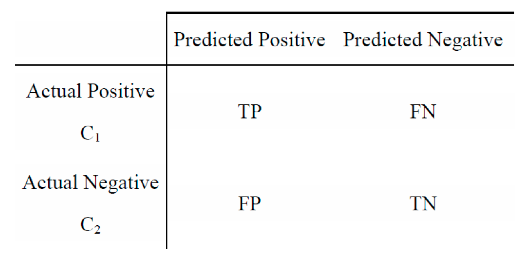
In the case of two-class problems, drawing a confusion matrix (Figure 2) would help visualize the theory. The performance of machine learning algorithms is also typically evaluated by a confusion matrix.

In the confusion matrix, TN is the number of negative examples correctly classified (True Negatives), FP is the number of negative examples incorrectly classified as positive (False Positives), FN is the number of positive examples incorrectly classified as negative (False Negatives), and TP is the number of positive examples correctly classified (True Positives).

To minimize the given wrong assignment approach, we divide the input space into decision regions (R_k), one region for each class (R_k is assigned to class C_k). While doing this operation, a mistake occurs when an input vector value belonging to R₁ is assigned to C₂ or a vector value belonging to R₂ is assigned to C₁. The equation given below used to calculate this mistake:

$$p\left(misclassification\right)={{\displaystyle \int }}_{R_1}^{}p\left(X, C_2\right).dx +{{\displaystyle \int }}_{R_2}^{}p\left(X,C_1 \right).dx$$

(2)

where:

• X is an input vector that consists series of values (a set of data),
• C₁ and C₂ are the two classes,
• R_k is decision regions,
• k is a constant that takes the value of 1 or 2.

To minimize misclassification, X must be assigned to the classes that have provided a smaller integral value.

To reducing the expected loss, assuming that for a new value of X, we assign it to class C_j whereas the real correct class is C_k. This means we have incurred a loss L_kj, which is the k, j element of the confusion matrix. The following equation gives the average loss function:

$$E \left[L\right]={\displaystyle \sum }_k{\displaystyle \sum }_j{{\displaystyle \int }}_{R_j}^{}{L}_{kj} p\left(X, C_k\right).dx$$

(3)

where:

• L_kj is an occurred loss value,
• X is an input vector that consists series of values (a set of data),
• C_k is the actual correct class,
• R_j is decision regions,
• j, and k is the constant of regions that take the value of 1 or 2.

The best solution is one that minimizes the average loss function. For a given input vector X, the uncertainty in the correct class is expressed through the joint probability distribution p(X, C_k).

The interpretation of the method under a short description of the STD presented as follows:

Predictive analysis, especially in machine learning classification, is tried to estimate the future possibility of an event in advance from the historical set of data related to that event. Simply the researcher needs the collection of data features to conduct the analysis. The reason for additional questions in any survey is to collect more information related to the subject issue.

It is common to perform a survey study to measure people’s opinions on a specific topic, and all surveys have a set of questions for different analysis purposes. This case study’s prime concern is to ask a correct set of questions related to the mobility preferences of university students of a rural town in a proper way while respecting their sensitivities. Therefore the structure of the questions did not contain any political or misleading contents.

The initial attempt with direct questioning is intended to test the responder’s reaction to demanding more PBS in daily life and resulted in an outcome below what is typically expected. This situation displays the influence of a status quo that we mentioned earlier. The status quo that the sustainability and availability of PBS in Japan’s rural regions have been in a continuous declining state for a long time. This method is an attempt to discover the consequences of this condition to current-day mobility demands.

The secondary questioning regarding the same problem is intended to discover a concrete development in the responder’s mind. However, it is still not enough to measure other daily life indicators’ impact. Therefore, to collect more information about the PBS demand, three sets of questions, a demographical background, travel behavior, and overall life satisfaction prepared and asked the participant.

Many factors can affect anyone’s daily life mobility needs. In this case, those factors’ weight implications to the overall mobility requirement are intended to reveal. In this way, this method could explain the reasonability of any increase or decrease in predicting a specific issue.

Although there are numerous other types of classifiers in machine learning, the character of data type and the size of data are of the utmost importance to choose one effective classifier for the desired purposes. For this case, before proceeding any further, the collected data analyzed and processed statistically to better understanding.

Therefore, by the formal definition of the STD, this methodology is divided into three stages to analyze the current PBS situation in Japan’s rural city of Kitami. First, we surveyed university students’ demand rate regarding the current PBS. After completing the survey section, we proceeded with the statistics and hypothesis test to understand the data’s characteristics. Finally, we used the data as input to develop a machine learning prediction model based on STD to discover the potential of the user’s best demand rate for PBS.

3.2. Data

The data was collected through a 2019 questionnaire titled “Student daily life after school hours” conducted at Kitami Institute of Technology, where approximately 1800 undergraduate students are enrolled [76]. The information bulletin regarding the survey was spread all around the campus, and the data collection period took a month. Responders accessed the web link of an online form by reading the QR code on the notification form with the QR code reading feature of a free application for instant communication on their smartphones. The survey questions collected information about students’ demographics, transport preferences, and overall satisfaction with their academic life. The survey was responded to by 250 students, in other words, 14% of the student population.

Usually, surveys with low response rates and nonresponse bias raise a notable concern. In survey sampling, bias refers to the tendency of a sample statistic to systematically over-or under-estimate a population parameter. In theory, the optimum way to identify bias in the estimates from a sample of respondents would be to compare the estimates to actual population values; however, population values are not always available [77].

Furthermore, a survey’s response rate reflects the collected data quality and reliability as an essential indicator. Since there is no agreed-upon minimum acceptable response rate, it largely depends on creating, distributing, and managing the surveys [78].

A conducted study in Japan found evidence of response rate bias for univariate distributions of demographic characteristics, behaviors, and attitudes. Still, during examining relationships between variables in a multivariate analysis, controlling for various background variables, findings do not suggest bias from low response rates for most dependent variables [79]. Moreover, the survey environment, how questions are asked, and the respondent’s state define problems in measurements. For instance, when we analyze data from another survey study focusing on the health-promoting lifestyle profile of Japanese university students, we see that the response rate decreases as the student year increases [80]. Nevertheless, in our case, absolute reliability can only be provided by applying the same questionnaire to new students enrolling each year in university and comparing the results obtained. However, at present, the distribution of sex and origin of responders generated by this survey data also matches the current student population characteristics.

There are also statistical formulas available for determining the size of the sample [81]. The two critical factors for these formulas are the margin of error (in the social research, a 5% margin of error is usually acceptable) and the level of confidence that the survey findings’ results are accurate (the typical confidence levels used are 95 %) [82].

The size of the collected responses and total student population calculates the margin of error as ±5.76% with a 95% confidence level. A 95 percent confidence level means that 95 out of 100 samples will have the actual population value within the specified margin of error of ±5.76 percent.

The obtained response rate from the student survey still encouraged us to exhibit the differences and similarities in the student community of the university town of Kitami within a given limit.

The urban outline of Kitami city is distributed sparsely, with winter periods mainly being cold and snowy compared to the rest of Japan [83]. The university campus area is 2.5 km from the city center. Transportation in Kitami city is highly automobile-dependent (152.4 automobiles per 100 people) [84], which is much higher than the average of the whole Hokkaido prefecture (68.67 automobiles per 100 people) [85]. The offered frequency of PBS is relatively limited due to a lack of passengers’ interest, e.g., some bus lines run only 3 or 4 times per day. The main bus line, running across the city, runs four times per hour and ends around 21:00 on weekdays and 20:00 on weekends [86].

University students in Kitami city come from various parts of Japan, with only 35% from Hokkaido prefecture, and the ratio of female students is 14 % [87]. In other words, students from different prefectures represent an active population of domestic tourists for locals and business owners, at least until they graduate from the university. The broad impact of a society with a declining birthrate, such as Japan, although not noticeable around big cities, significantly influences the local economy in rural towns such as Kitami. Therefore, it is crucial to engage young people living in this city to support the local economy from various perspectives. The idea includes both purely economic aspects such as buying from local stores and economic and environmental aspects, such as choosing PBS in favor of private cars.

We have decided to use a two-step verification process in the survey design under the conditions mentioned above. Because the long-neglected status of PBS in rural Japan has reinforced the belief that there will be no change in the situation, psychologically, people have come to accept this as the status quo.

The first question we asked (first inquiry—FI) was whether a student would like to use PBS more in the current situation with a binary response (yes/no).

The following several questions we asked for linked the daily life activities that need mobility, including joining a part-time job, dinner options, nearby restaurant demand, and supermarket shopping. Next, we asked questions regarding the respondents’ public transport behavior, such as frequency of using PBS, days and times they prefer to go out, the transportation type they choose during these activities. These questions aimed to demonstrate to the responders the essential requirement of PBS in daily life.

The second question we asked (second inquiry—SI) was whether a student would like to use PBS in an alternate situation with a binary response. An alternate PBS that can provide the mobility need of any person during everyday life for various reasons such as going shopping, dining in a restaurant, traveling for sightseeing purposes, or even conveniently commuting to part-time job workplaces.

The difference in responders’ decision distribution between the two groups (Yes/No) did not reveal any visible diversity in the first inquiry (FI); however, the second inquiry (SI) resulted in a meaningful difference. This finding showed that using the two-stage verification probe was the right decision to analyze this specific community.

Furthermore, the variable identified with the second inquiry (SI) became the entire survey study’s target value for the machine learning-based predictions. Finally, regarding the various questions asked, the respondent’s overall satisfaction with academic lives has also been reviewed.

By the end of data collection, we populated 18 different types of categorical variables from the respondents. The conversion of these 18 categorical variables to the continuous type resulted in 47 types of continuous labels.

Once the dataset was formed and prepared for the analysis, chi-square statistical tests were applied to determine the best subset collection while dataset attributes were of the categorical value form. The chi-square test is a nonparametric statistical test that measures the association between two categorical variables [88]. It is not applicable to analyze parametric or continuous data types [89].

Additionally, the p-value calculation was applied while dataset attributes were of the continuous value form. Statistical significance is the probability that the observed difference between two groups is due to chance. If the p-value is more significant than the statistical significance level (α), any practical difference is assumed to be explained by sampling variability. However, reporting only the significant p-value for analysis is not adequate to fully understand the effect sizes [90,91].

Due to differences in the perception of statistical inference to prevent misinterpretation of evidence from the given data [92], we set two different criteria to evaluate the participants’ behavior better and simplify the models’ predictive weight. These criteria were chi-square and p-value.

3.3. Hypothesis Test

As described above, we compared participants’ responses (positive or negative) to two different stimuli by conducting a two-step verification probe in the survey. We measured these two stimuli with two separate survey questions: the first inquiry (FI) and the second inquiry (SI). A sample result is applied to a 2 × 2 contingency table (

Table 1. Sample of a 2 × 2 contingency table.

	Trial 2 Positive	Trial 2 Negative	Row Total
Trial 1 Positive	A	B	A + B
Trial 1 Negative	C	D	C + D
Column Total	A + C	B + D	N

), which tabulates the outcomes of two trials on a sample of N subjects.

There were four cells in the table named A, B, C, and D. Cells A and D hold the concordant results (the frequency of individuals who answered positively or negatively to both stimuli). Cells B and C contain the discordant results (the frequency of individuals who responded positively to one stimulus but negatively to the other) [93].

The critical issue here was whether the totals in these two discordant cells were sufficiently different to suggest that they trigger different reactions. In terms of the null hypothesis testing paradigm, this could be explained by a p-value, which is the probability of seeing the observed difference in these two discordant values. The statistical test designed to provide this probability is McNemar’s test [94]. Both B and C values were used in the given formula below to calculate the test [95].

$$X^2=\frac{{\left(B-C\right)}^2}{B+C}\approx \frac{{\left(\left|B-C\right|-0.5\right)}^2}{B+C}$$

(4)

where:

• X² is a chi-squared distribution with 1 degree of freedom,
• B is the frequency of individuals who responded positively to the first stimulus but negatively to the second,
• C is the frequency of individuals who responded negatively to the first stimulus but positively to the second.

McNemar’s test compares two dichotomous variables’ marginal homogeneity as part of the chi-square statistic. It is preferable for analyzing paired binomial data to conclude if there is a meaningful change in the data between two stimuli. Additionally, for understanding the influential association between two dichotomous variables, Cramér’s V (other naming is Cramér’s phi and denoted as φc) value can also be calculated. Cramér’s V correlation varies between 0 and 1 [96].

A hypothesis test gives a fair settlement between two mutually exclusive statements. The definition of our hypothesis testing is denoted as follows:

• H0: µ₁ = µ₂;
• H_A: µ₂ > µ₁;
• H₀—The null hypothesis states that there is no difference concerning PBS requests between the regular days (µ₁ = mean of FI) and weekend days (µ₂ = mean of SI) during the 20:00–24:00 h by university students in the Kitami city;
• H_A—The alternative hypothesis states that there is a difference.

The statistical significance level (α) for this study was also chosen before the data collection and set to 5% (0.05) [97].

3.4. Predictive Modeling

The predictive modeling part explains the applicability of an inferential model for data mining algorithm to predict new or future observations. In particular, the goal is to predict the output value (y) for recent statements given their input value sets (X) [98]. In predictive modeling, we used a group of classifiers trained with the dataset to predict whether a randomly selected student would prefer to use PBS more or not.

Classification is a part of predictive modeling, and it is an integral part of the data science processes. A typical supervised statistical learning problem is defined when the relationship between a response variable and an associated set of predictors (inputs) is of interest while the response variable is categorical. One challenge in classification problems is to use a dataset to construct an accurate classifier that produces a class prediction for any new observation with an unknown response [99].

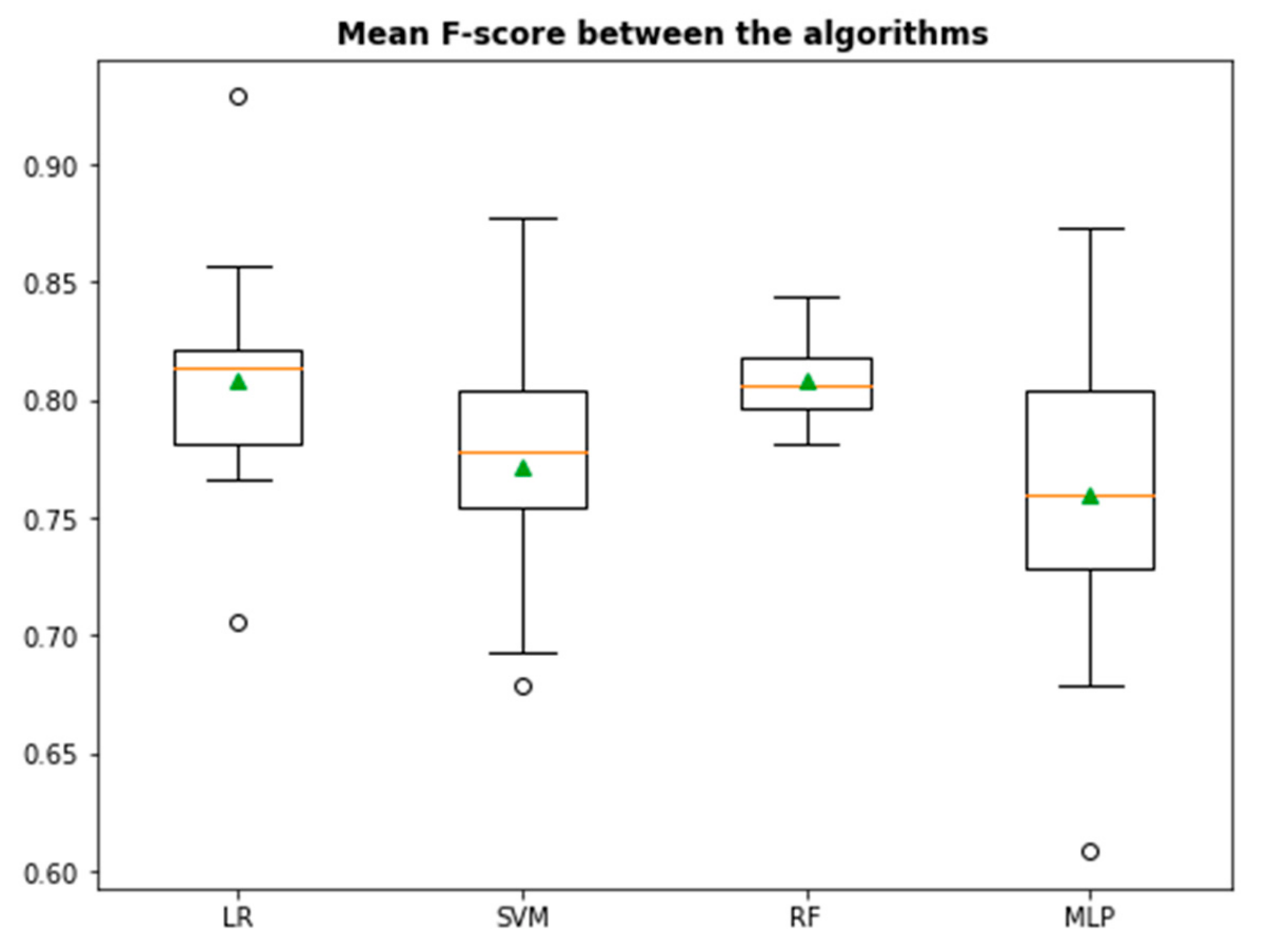
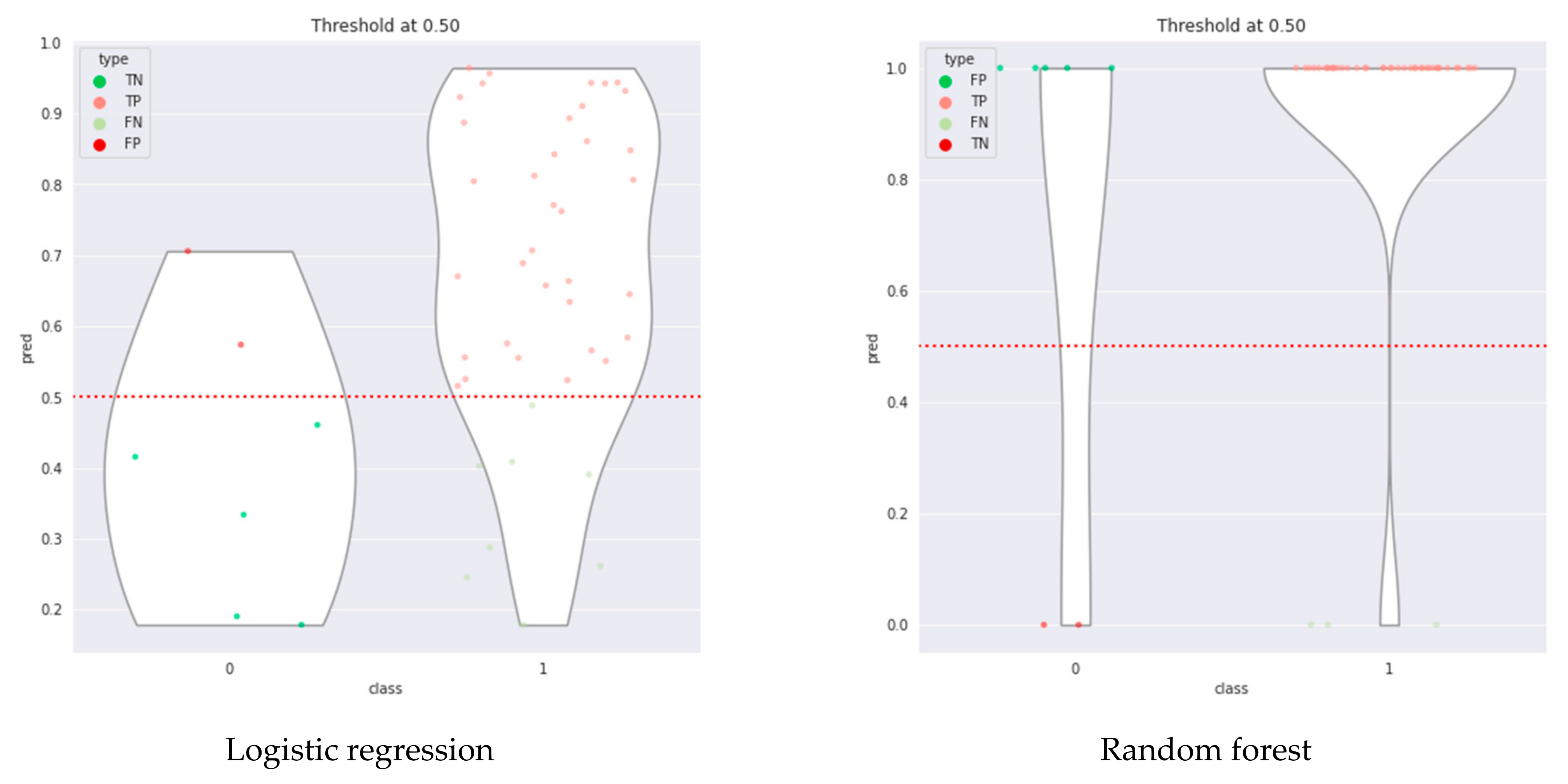
The classifier algorithms used for comparison in our research included a logistic regression (LR), a support vector machine (SVM), a random forest (RF), and a multi-layer perceptron classifier (MLP).

Logistic regression is considered a standard approach for binary classification in the context of a low-dimensional dataset. This condition usually occurs in scientific fields such as medicine, psychology, and social sciences, where the focus is not only on a prediction but also on explainability [100]. LR classifier aims to test the relationship between a categorical dependent variable and continuous independent variables by plotting the dependent variables’ probability scores. LR models develop from the statistic that best explains the relationships with yes or no answers (no answer indicates missing data) [101].

SVMs do separate two classes in the data space by building a decision boundary [102]. The SVM classifier creates a maximum-margin hyperplane that lies in transformed input space and splits the class samples while maximizing the distance to the nearest dividing samples [103].

RFs are a machine learning technique that aggregates many decision trees in the ensemble (this is often called “ensemble learning”), resulting in a reduction in the variance compared to single decision trees [104]. The objective behind an RF classifier is to take a set of high-variance, low-bias decision trees and transform them into a low variance and low-bias model. By aggregating individual decision trees’ various outputs, RF reduces the conflict that can cause errors in decision trees. RF also allows a reliable assessment of the importance (weight) of each variable.

Unlike previous classification algorithms, an MLP relies on an underlying neural network to perform classification. Artificial neural networks try to learn tasks (to solve problems), applying the similarities to the brain’s behavior. Specifically, similarly to how the brain is composed of a large set of specialized cells called neurons that memorize brain activity patterns, neural networks memorize patterns between features to fit as closely as possible to the desired output. MLP is often achieving high performance. However, similarly to how it is difficult to explain the behavior of separate neurons in the brain, neural network-based models are also considered ill-suited for explanatory modeling, especially when the training data size is small [105,106].

The performance of machine learning algorithms usually is evaluated by predictive accuracy. However, this is not appropriate when the data is imbalanced, and the costs of different errors vary markedly. Often real-world datasets are predominately composed of “normal” examples with only a tiny percentage of “abnormal” or “relevant” examples [107].

The dataset was split into the train (80%) and the test set (20%). We used test sets, which the model did not see, during the performance metrics calculation to avoid over-optimistic predictive accuracy. After interpreting the performance metrics, the method that produces the most compatible outcome with the real-life situation was compared.

The performance metrics for evaluating each algorithm in this study were the F-measure (Fβ), accuracy, area under the curve (AUC), Cohen’s kappa, and cross-validation (CV).

F-Measure is a commonly used performance measure and is more informative about the effectiveness of a classifier on its predictive ability than simple accuracy. The β in Fβ sets different weightings for Precision and Recall (β = 1 or 2 or 3). We therefore computed the F1 score, where β was chosen to be equal to 1. Accuracy is not suitable considering a user preference bias toward the minority (positive) class examples because of the least represented impact. However, more actual examples are reduced when compared to that of the majority class. Two other popular measures used, especially in imbalanced class domains, are the receiver operating characteristics (ROC) curve and the corresponding area under the ROC curve (AUC).

Moreover, ROC curves do not provide a single-value performance score, which motivates the use of AUC. The AUC allows the evaluation of the best model on average. Still, it is not biased toward the minority class [108].

The reliability of data collection is an essential component influencing the overall real-life utility of the proposed machine learning model. Cohen’s kappa statistic is frequently used to test interrater reliability, which shows how reliable the data is. Cohen’s kappa was developed to account for the possibility that raters guess on at least some variables due to uncertainty. A kappa is a form of the correlation coefficient. Correlation coefficients cannot be directly interpreted, but a squared correlation coefficient, called the coefficient of determination (COD), is directly interpretable. The COD is explained as the amount of variation in the dependent variable that can be explained by the independent variable [109]. Like most correlation statistics, the kappa can range from −1 to +1.

Cross-validation (CV) is a popular strategy for algorithm selection. The main idea behind CV is to split data, once or several times, for estimating the risk of each algorithm. Part of the data (the training sample) is used for training each algorithm, and the remaining part (the test sample) is used for estimating the efficacy of the algorithm. In the process of CV, the algorithm with the highest efficacy is then selected. CV is a widespread strategy because of its simplicity and universality [110].

4. Case Study and Results

4.1. Data Analysis

This section discusses the data presented in three parts as the tables. Part A represents students’ demographic background, Part B discusses students’ travel behavior, and Part C analyzes students’ overall satisfaction. Additional explanations regarding the abbreviation used in the tables are provided in Appendix A.

The way to interpret Chi² column in the tables is that categorical features with the highest values for the chi-squared statistics indicate higher relevance and importance in predicting students’ PBS demand. On the other hand, after converting data to continuous type, the p-value is the evidence against the null hypothesis. The smaller the p-value is, the more statistically significant the evidence.

4.1.1. Part A—Students’ Demographic Background

In this part, we analyzed the survey part where the respondents were asked to provide their demographic background. The results are presented in

Table 2. Descriptive differences of students’ demographic background.

No	Attributes	No	Label Name	Relative (%)	Chi2	p-Value
1	Sex				0.18
	Female	1	SexF	14.8		0.27
	Male	2	SexM	85.2		0.27
2	Origin				0.11
	Japan, other than Hokkaido	3	“OJ”	58.8		0.98
	Hokkaido	4	“OH”	33.2		0.42
	International	5	“OI”	8		0.15
3	Accommodation				0.65
	Apartment	6	“Lapart”	67.2		0.39
	Boarding house	7	“Lblodge”	17.2		0.35
	University dormitory	8	“Ldorm”	8.8		0.78
	Parent’s home	9	“Lhome”	6.8		0.60
4	Preferences of Dinner				0.58
	Cooking	10	“Dcook”	54.4		0.63
	University cafeteria	11	“Dcafe”	20		0.13
	Meal served by a boarding house	12	“Dbmeal”	18.4		0.38
	Lunch box	13	“Dbento”	5.2		0.26
	Restaurant	14	“Drstrnt”	2		0.13
5	Participation in a part-time job	15	“PTime”		2.99	0.01
	Yes			52
	No			48

:

Among the 250 respondents who participated in the survey, 85.2% were males, and 14.8% were females. Regarding the origin, 33.2% of the students were from the Hokkaido region, 58.8% from other parts of Japan, and 8% were foreigners. Regarding the students’ distribution of accommodation, 67.2% resided in an apartment house (block of flats), 17.2% resided in boarding houses with a meal, 8.8% resided in a university dormitory, and 6.8% were staying with their own family. The preferences of dinner, while 54.4% of the students said they cook for themselves, 20% had their dinner at the university cafeteria, 18.4% at the boarding house (while some boarding house near the campus also offers two meals a day even for a non-tenant), 5.2% were buying their meals/lunch boxes at convenience stores, and only 2% used the restaurants nearby. The ratio of students taking part-time jobs was 52%.

The prime finding in this part is that participating in a part-time job by the 52% of respondents has created the highest values for the chi-squared statistics and provided the lowest p-value. In other words, in Kitami city, university students provide a significant economic value not only by being a student but also by participating in the local business job market.

4.1.2. Part B—Students’ Travel Behavior

In this part, the respondents were asked to provide their travel behavior. The results are represented in

Table 3. Descriptive differences of students’ travel behavior.

No	Attributes	No	Label Name	Relative (%)	Chi2	p-Value
6	Frequency of public buses usage				4.30
	Daily	16	“PTFD”	8		0.15
	Weekly	17	“PTFW”	30		0.00
	Monthly	18	“PTFM”	30.4		0.80
	Less than a Month	19	“PTFL”	31.6		2.41
7	Possession of an automobile	20	“Car”		0.3	0.55
	Yes			14.4
	No			85.6
8	Demand to use buses more often	21	“FI”		17.95	0.00
	Yes			59.6
	No			40.4
9	Preferred evenings to go out mostly		(multi-selection)
	Friday	22	“Frdy”	32.4	4.47	0.01
	Saturday	23	“Strdy”	84	0.12	0.38
	Sunday	24	“Sndy”	69.6	0.94	0.08
10	Preferred periods to go out mostly		(multi-selection)
	18:00–20:00	25	“HL”	76.4	0.00	0.94
	20:00–22:00	26	“HM”	36.8	4.13	0.01
	22:00–24:00	27	“HH”	26	7.41	0.00
11	Preferred transport types during that period				1.09
	Walk	28	“PTTwalk”	45.2		0.26
	Bicycle	29	“PTTbike”	21.2		0.62
	Bus	30	“PTTbus”	15.6		0.20
	Personal automobile	31	“PTTcar”	12.8		0.13
	Taxi	32	“PTTtaxi”	5.2		0.08
12	Demand for buses in that period	33	“SI”	(target value)
	Yes			70.8
	No			29.2

:

The frequencies of using public buses to travel to other areas than the university campus resulted in 62% monthly or less than a month. The student’s automobile ownership was rated at 14.4%. Among the participants, 59.6% requested more PBS opportunities with a 6% margin of error (95% confidence interval). Friday, Saturday, and Sunday collected, respectively, 32.4%, 84%, and 69.6% of the students’ interest in most favorite days to go out. The favorite time interval was between 18:00 and 20:00 and accumulated the interest of 76.4% of the students. The time between 20:00 and 22:00 was selected by 36.8% of the students, and the time between 22:00 and 24:00 was selected by 26% of the students. During these periods, the students’ transportation choices were as follows: 45.2% preferred to walk, 21.2% preferred bicycle, 15.6% preferred public bus, 12.8% preferred their own car, and 5.2% preferred taxi as a transportation option. In this circumstance, a second confirmation of the demand for PBS resulted in a 70.8% agreement of responders with a 5.6% margin of error (95% confidence interval).

The prime findings in this part are the high percentage of walk preferences. The reason for the high rate of walk preferences was that the bus line was not available. In some bus lines, passengers still have to walk halfway to the destination, so many prefer to walk instead of paying for bus fees. With the given student car ownership being 14%, it is evident that a personal car-dependent public transport model does not cover most students in this local city. Especially weekly bus users, who want to use buses more regularly, or those who want to go out on Friday night after 20:00, and who need to use a taxi in this situation created the highest chi-square stats and p-value correlation.

4.1.3. Part C—Students’ Overall Satisfaction

In this part, the respondents were asked to provide their overall satisfaction with their academic life and future expectations. The results are presented in

Table 4. Descriptive differences of students’ overall satisfaction.

No	Attributes	No	Label Name	Relative (%)	Chi2	p-Value
13	University’s contribution to the city				1.32
	Economically	34	“Conteco”	34.8		0.10
	Educationally	35	“Contedu”	26		0.76
	Academically	36	“Contaca”	19.6		0.65
	Industrially	37	“Contind”	16		0.03
	Culturally	38	“Contcul”	3.6		0.08
14	Evaluation of the university				0.53
	High	39	“ValueH”	19		0.54
	Medium	40	“ValueM”	34		0.26
	Low	41	“ValueL”	47		0.55
15	Winter seasons negative effect on the daily life				5.63
	High	42	“WinterH”	64		0.01
	Medium	43	“WinterM”	22		0.15
	Low	44	“WinterL”	14		0.08
16	Demand a fast-food restaurant nearby campus	45	“Mc”		1.39	0.00
	Yes			83.2
	No			16.8
17	Demand a nearby supermarket	46	“SpM”		0.77	0.00
	Yes			90.4
	No			9.6
18	Dwelling in the same city after graduation	47	“Grad”		0.04	0.84
	Yes			20
	No			80

.

Regarding the university’s contribution to the city from the students’ point of view, 34.8% of the participants expressed the importance of economic contribution, 26% highlighted the educational contribution, 19.6% chose the academic contribution, 16% industrial, and only 3.6% cultural. Students’ university rating into three scale bins resulted in 47% for low, 34% for medium, and 19% for high. The negative effect of winter seasons on students’ daily lives resulted in 64% of replies for high, 22% for medium, and only 14% for low. The idea that “Having at least a chain restaurant (for example, McDonald’s) near the campus area would make life more comfortable” resulted in support of 83.2%. Similarly, the idea that “Having a supermarket near the campus” resulted in 90.4% of the students’ interest in favor. Finally, with regards to the question of “Would you stay in Kitami city after graduation if there were any career opportunities for you?” 80% of participants selected a negative response, while 20% answered positively to this question. The positively answered students group divided by 40% from Hokkaido origin, 46% from another part of Japan, and 14% were international students.

The facts emerging in this section can be summarized as follows: the university’s contribution to the city does not represent any common consensus among the participants. Participants generally rate the university at an average level. Participants who found the negative impact of the winter season highly on daily life achieved a high value in the chi-square test while at the same time providing the lowest p-value. Likewise, the need for a chain restaurant and a supermarket nearby perceived support from the overwhelming majority of participants. Both variants were statistically verified by producing a low p-value. Another important finding is that roughly 4 in 5 participants do not want to settle in Kitami city after graduation. On the other hand, the remaining 20%, if extrapolated to the whole student population, result in about two hundred people per year, which represents a vital and robust workforce that, if given the opportunity, could invigorate the decreasing population of Kitami.

4.2. McNemar’s Test

The contingency table created from our dataset is represented in

Table 5. 2 × 2 contingency table.

FI/SI	Second Inquiry (SI)—Yes	Second Inquiry (SI)—No	Row Total
First Inquiry (FI)—Yes	129	20 (B)	149
First Inquiry (FI)—No	48 (C)	53	101
Column Total	177	73	250

. Cell (B) represents the number of students who were willing to use public bus services at the initial survey but changed their minds in unfavorable of bus services during the second survey. Cell (C) represents the number of students whose case is the opposite.

The calculated result of the test is presented in

Table 6. The result of McNemar’s Test.

Set of Parameters	Value
McNemar’s Chi-square (1.0)	11.5294
p-value	0.0007
Cramér’s V	0.2148

[111].

The statistical significance level (α) for this study was also chosen before the data collection and set to 5% (0.05). The decision was statistically significant; we are 95% (0.95) confident that it would be implausible to have occurred, given the null hypothesis is valid. Hence, the null hypothesis can be rejected in favor of the alternative hypothesis. Cramér’s V correlation with a value of 0.2148 indicates an influential association between the variables.

Additionally, the students’ decision change populated by groups regarding the transportation option during their preferred period in the existence of PBS is given in

Table 7. The student’s decision change regarding the transportation preferences by groups.

Cell Group	Bike	Bus	Car	Taxi	Walk	Row Total
A	30	24	9	9	57	129
B	5	3	1	0	11	20
C	9	7	10	3	19	48
D	9	5	12	1	26	53
Column total	53	39	32	13	113	250

.

In Figure 3. The member of group B and group C were represented in the radar charts. Decision changes mainly occurred among the respondents who prefer to walk, and this response also covers the majority of the student population.

The findings suggest that it could be helpful in the city to increase the PBS frequencies, at least for the students’ periods as most desirable (e.g., Friday and Saturday evenings after 20:00 h).

4.3. Classification

Below, we report on the results from four machine learning classifiers (logistic regression, support vector machines, random forests, and artificial neural networks) to predict the binary demand variable based on the features described in Section 4.1. We report performance measures on a 20% random sample of test data in all experiments. With the remaining 80% of the data, we use 10-fold cross-validation to tune the model parameters. These parameters were the regularization strength and solver function for logistic regression, the number of iterations in support vector machines, the tree’s depth in random forests, and hidden layer size in neural networks.

Before moving on to the broader review, we took a pragmatic experiment with the subset selected in the student’s dataset. The feature selection technique is an essential process in machine learning, where the set of all possible features is reduced to those required to contribute most to the prediction output [112]. We used SelectKBest as a popular feature selection method [113]. SelectKbest is a feature selection algorithm used to improve prediction accuracy or increase performance on high-dimensional datasets [114]. As the definition suggests, this method is ideal for high-volume data sets, and SelectKBest removes all but the K highest scoring features [115]. The best predictors obtained by SelectKBest are given the

Table 8. Selected top 10 features of SelectKBest techniques.

	1	2	3	4	5	6	7	8	9	10
Label	FI	PTFL	PTFW	HH	Frdy	HM	Contind	Contcul	PTime	PTTtaxi
Chi2 Score	17.940270	11.884577	9.133065	4.131003	4.470251	4.131003	3.901401	3.023923	2.987147	2.908807

. Additional explanations regarding the abbreviation used in the table given in Appendix A.

However, the effect of the significant number of features determined by SelectKBest on the classification model’s accuracy was not as high as expected, with a 0.74 value of accuracy. Nevertheless, these are factors that come at the forefront of situations in which students feel the need for PBS, in their opinion.

Therefore, as we explained above, due to the relatively small volume of students’ data density, we preferred to use all dataset features and considered their effects on the estimation depending on each label’s separate correlation over the target variable.

The shape of the data has changed by creating dummy variables to cast categorical variables to continuous applicability in the classification processes. The dataset’s shape consists of 250 records and 46 features for prediction. Next, the data were normalized, and models were fitted.

The evaluation metrics for normalized data prediction are shown in

Table 9. Prediction metrics for classifiers with the normalized data.

Classifier	F-Measure	Accuracy	AUC	Cohen’s Kappa	Cross-Validation F1
Logistic Regression	0.88	80%	0.81	0.39	0.82
Linear SVM	0.80	70%	0.71	0.25	0.76
Random Forest	0.91	84%	0.61	0.25	0.81
MLP	0.67	56%	0.68	0.17	0.76

. The performance was comparable across models (AUC between 0.81 and 0.68). The differences at the Cohen’s kappa metrics with modest gains in the case of logistic regression were decisive. A higher accuracy value with the training set might indicate overfitting. For this reason, the test set accuracy is more relevant for evaluating the performance on unseen data since it is not biased. As we mentioned before, the MLP classifier performs the worst due to the relatively small data size.

On the other hand, the random forest algorithm provided the highest prediction results on F-measure. Furthermore, the log-loss (cross-entropy loss) marks a logistic regression classifier’s performance and gets the best of its value near 0. In this model, it was 0.48.

As seen from the table, the logistic regression and random forest algorithms are preferable for practicality and reliability. Those algorithms are often used with data mining growth in the information systems domain [116,117]. The powerful strategies among the metrics here were Cohen’s kappa results. In addition, cross-validation may lead to higher average performance than applying any single classification strategy, and it also cuts the risk of poor performance in practice [118].

In Figure 4, a graph for mean F-scores between the algorithms was given to perform a 5 × 2 cv paired t-test procedure to compare the performance of the two models [119]. According to Figure 4, logistic regression and random forest classifiers perform better than the other algorithms. We assume a significance threshold of α = 0.05 for rejecting the null hypothesis that both algorithms perform equally well on the dataset and the result of conducted the 5 × 2 cv t-test given below:

• The p-value is = 0.528
• The t-statistics is = −0.678

Since p > α, we cannot reject the null hypothesis and conclude that the two algorithms’ performance is not significantly different.

For visualization purposes, a set of graphs for class distribution of logistic regression and random forest classifiers was given below in Figure 5.

Finally, we have able to define around 80% of the reliable variation in selecting night hours and optimized PBS with all survey dataset features. In addition, classification is a practically applicable method. Policymakers can use this method to estimate the demand each year and change the PBS accordingly.

5. Conclusions

5.1. Discussion of Research Finding and Limitations

The available research study on public buses in rural areas or small cities in Japan is limited but expanding. The characteristics of rural areas or small towns have encouraged private cars, which has caused problems for the continuity of public bus operation due to financial feasibility. There are two main reasons people were indifferent and reluctant to use the bus. The first one is the limited number of buses, and the second one is the operational time [120]. Another major problem is the accessibility of the bus stops. A significant statistic revealed by a survey aimed to measure people’s bus use intention in Japan’s rural city. Nearly half of the respondents live within five minutes of a bus stop, and approximately 80% of them are within 10 min of a bus stop [121]. In addition, the common point of the studies is that if the demand is supplied appropriately, the tendency of people to use buses instead of personal cars increases.

In the presented study, we endeavor to highlight why and how rural city university students’ transport quality needs to be improved based on demand.

However, if we desire this method to be positioned in a more generalized frame, it must respond to some conditions:

First, the sample size of a population is essential to prevent any scientific suspicion of the significance of the statistic’s accuracy behind the research. The sample size of 250 students from a population of 1800 is notable but less than satisfying the exact expected confidence level (a fair 5% margin of error for a population of 1800 persons requires 317 responses with a population proportion value of 50%). The obstacle for this task is the low response rate in Japan. Social and economic status can affect the answer rate; for instance, voter turnout, a measure of citizens’ participation in the political process, was 53% during recent elections, lower than the Organization for Economic Co-operation and Development (OECD) average of 68% [122].

Second, the method provides a simple foresight into next year’s PBS demand projection from a year earlier student opinion poll. That means the method’s performance requires ensuring a data flow by obtaining new survey data from newly enrolled students each year. In this way, we can analyze the low response rate on reliability, non-random response model, and possible selection bias.

Third, PBS demand analysis was the main topic in this case study scenario. The method requires at least one more test with a different case scenario and a different topic.

On the other hand, the survey question design and order may need to be improved depending on each year’s new conditions that may help the city’s transportation bureaus manage their decisions more interactively to meet passenger demand with their services.

As researchers indicated in their detailed analysis in literature, improving university students’ mobility makes it easier for them to participate in more social activities after school hours, enhancing their socializing ability, which is a bit problem in Japan.

The findings for the three objectives of this research presented in Section 4.1, Section 4.2 and Section 4.3 can be summarized as follows:

• Initially, the current demand rate, measured at 60% with the two-step verification probe, was strictly compatible with the Japanese countryside’s real-life situation. The demand for PBS is relatively low. However, the secondary probing increased the demand rate to 71%;
• The initial and secondary probing findings were subjected to a hypothesis test to provide a fair settlement between two mutually exclusive statements. The final decision was confirmed statistically and significantly supported the hypothesis that there is a need to improve on the PBS to fulfill students’ mobility demand based on the collected student data sample;
• After implementing several machine learning-based prediction methods to measure whether the increase in demand would occur, the best and most reliable prediction of the demand settled at 80%. Additionally, with a simple series of questions (Appendix B), we have explained a variation of 20 percent that can increase demand for PBS.

Providing sustainable and reliable information is a fundamental requirement of decision-making. Researchers collect and process data systematically, unbiased, and solution-oriented to help policy-level decision-makers make practical decisions [123]. Our research could help decision-makers generate more practical and realistic policies regarding optimizing the public bus service frequencies.

The following steps in our research will involve:

• Discussions with university administrators;
• Improving our predictive models with enhancing daily life indicator variations;
• Possibly expanding our method applicability to a research field other than public bus transportation.

5.2. The Current Policies and Implications

In a general term, there is always a requirement for statistics produced by various methods, including survey statistics, to properly understand a regions’ actual transport and traffic limitations. For instance, the PBS usage continuously decreases around 36% over the past 20 years in Japan except for its three major metropolitan areas Tokyo, Osaka, and Nagoya [124]. Based on this statistical information, a general assessment of the current and suggested solution-oriented policies for promoting PBS versus private vehicle can be summarized as follows:

• On-demand transportation services, such as autonomous shuttles, can operate more economically under an uncertain demand level;
• Micro-mobility solutions, such as e-bikes for students and tourists and e-wheelchairs for the elderly, can meet public transportation requirements.

A demand-based and situation-specific solution may be convenient for rural municipalities with different geographical, cultural, and population characteristics. As in this study, hosting a university is a good thing for a city’s economy, but not every rural city may have this privilege.

Instead of using personal vehicles, promoting using more current public transport instruments while they are still operating is also an effective way in the circumference of the existing situation eventually. Simultaneously, when the passenger demand increases toward the public transport, the services’ frequency and quality increase.

The studies are ongoing to realize the future applicability of mobility as a service in Japan. It has featured the necessity of providing data covering the whole country by standardizing transport operators’ data into a standard format and making it open data [125].

Improved autonomous vehicles providing a promising solution to passenger transportation problems in rural areas might drastically change the transportation arena. However, there are situations where autonomous vehicles will not meet transport expectations. For instance, autonomous vehicles have difficulties operating in poor weather, such as fog and snow, and reflective road surfaces from rain and ice create other challenges for sensors and driving operations [126].

In an ongoing study, Higashihiroshima City is conducting an experimental project in collaboration with private initiatives that aim to solve traffic problems around Hiroshima University, providing a loop bus service and collect data for the future automated driving society [127]. As in this case, a fixed-route loop bus through areas that lacked regular access to existing public transit can be a sample of best practices.

Finally, this research presented that public transportation is essential for a community to carry out daily life activities based on mobility. If it is chosen more often by the students and other citizens (such as travelers, domestic tourists, and the elderly, who account for a large part of the city population), it will become more comfortable. Reversibly, in equilibrium, the quantity of a good supplied by producers equals the amount demanded by consumers [128]. The revitalization of local industries, needed especially in the post-COVID-19 pandemic reality, also depends on the enrichment of different transportation options.

References

1. Luczak, D.; Avary, M. Transforming Rural Mobility in Japan and the World. White Paper. World Economic Forum: Cologny, Switzerland. Available online: https://www.weforum.org/whitepapers/transforming-rural-mobility-in-japan-and-the-world (accessed on 16 January 2020).
2. Schofer, J.L. Routes to the future of urban public transit. Urban Aff. Q. 1983, 19, 149–166. [Google Scholar] [CrossRef]
3. Walters, A.A. Costs and Scale of Bus Services; World Bank Staff Working Paper No. 325; The World Bank: Washington, DC, USA, 1979. [Google Scholar]
4. Sakai, K. Public transport promotion and mobility-as-a-service. IEICE Trans. Fundam. Electron. Commun. Comput. Sci. 2020, E103.A, 226–230. [Google Scholar] [CrossRef]
5. Hoerler, R.; Stünzi, A.; Patt, A.; Del Duce, A. What are the factors and needs promoting mobility-as-a-service? Findings from the Swiss Household Energy Demand Survey (SHEDS). Eur. Transp. Res. Rev. 2020, 12, 1–16. [Google Scholar] [CrossRef]
6. Kawasaki, S. The challenges of transportation/traffic statistics in Japan and directions for the future. IATSS Res. 2015, 39, 1–8. [Google Scholar] [CrossRef] [Green Version]
7. Kato, H. Declining population and the revitalization of local regions in Japan. Meiji J. Political Sci. Econ. 2014, 3, 25–35. [Google Scholar]
8. Nghiêm-Phú, B. Japanese university students’ life satisfaction and their intentions to travel/study abroad. EJCJS 2015, 15, 10. [Google Scholar]
9. Takamatsu, R.; Min, M.C.; Wang, L.; Xu, W.; Taniguchi, N.; Takai, J. Moralization of Japanese cultural norms among student sojourners in Japan. Int. J. Intercult. Relat. 2021, 80, 242–249. [Google Scholar] [CrossRef]
10. Briedenhann, J.; Wickens, E. Tourism routes as a tool for the economic development of rural areas—Vibrant hope or impossible dream? Tour. Manag. 2004, 25, 71–79. [Google Scholar] [CrossRef]
11. Wilson, S.; Fesenmaier, D.R.; Fesenmaier, J.; Van Es, J.C. Factors for success in rural tourism development. J. Travel Res. 2001, 40, 132–138. [Google Scholar] [CrossRef]
12. Lane, B.; Long, P. Rural tourism development. In Trends in Outdoor Recreation, Leisure and Tourism; Gartner, W.C., Lime, D.W., Eds.; CABI Publishing: Wallingford, UK, 2000; pp. 299–308. [Google Scholar]
13. Chen, B.; Qiu, Z.; Usio, N.; Nakamura, K. Tourism’s impacts on rural livelihood in the sustainability of an aging community in Japan. Sustainability 2018, 10, 2896. [Google Scholar] [CrossRef] [Green Version]
14. Pereira Brando Albino, S. Tourism in University Cities. The Role of Universities in Place Branding. Ph.D. Thesis, University of Exeter, Exeter, UK, 2015. [Google Scholar]
15. Brennan, J.; Cochrane, A. Universities: In, of, and beyond their cities. Oxf. Rev. Educ. 2019, 45, 188–203. [Google Scholar] [CrossRef] [Green Version]
16. Llewellyn-Smith, C.; McCabe, V.S. What is the attraction for exchange students: The host destination or host university? Empirical evidence from a study of an Australian university. Int. J. Tour. Res. 2008, 10, 593–607. [Google Scholar] [CrossRef]
17. Eder, J.; Smith, W.W.; Pitts, R.E. Exploring factors influencing student study abroad destination choice. J. Teach. Travel Tour. 2010, 10, 232–250. [Google Scholar] [CrossRef]
18. John, S.; Hammond, R.; Keeney, L.; Raiffa, H. The hidden traps in decision making. Harv. Bus. Rev. 1998, 74, 47–58. [Google Scholar]
19. Kenichi, S. Feature: Railway management and the role of government, lessons from japanese experiences of roles of public and private sectors in urban transport. Jpn. Railw. Transp. Rev. 2001, 29, 12–18. [Google Scholar]
20. Calimente, J. Rail integrated communities in Tokyo. J. Transp. Land Use 2012, 5, 19–32. [Google Scholar] [CrossRef] [Green Version]
21. Eiichi, A.; Matsuhide, I.; Shinichi, K.; Yasuo, W. A History of Japanese Railways, 1872–1999; East Japan Railway Culture Foundation: Tokyo, Japan, 2000; Available online: https://www.ejrcf.or.jp/jrtr/history/index_history.html (accessed on 30 March 2000).
22. Yukihide, O. Feature: Restructuring railways, the backdrop to privatization in Japan—Successful “Surgical Operation” on Japanese railways. Jpn. Railw. Transp. Rev. 1994, 2, 2–9. [Google Scholar]
23. Ryohei, K. Feature: Big project financing, transportation investment and Japan’s experience. Jpn. Railw. Transp. Rev. 1997, 11, 4–12. [Google Scholar]
24. Mitsuhide, I. Feature: Rural railways, maintaining public transport in Japan’s countryside—Burden sharing and subsidies. Jpn. Railw. Transp. Rev. 1996, 9, 2–8. [Google Scholar]
25. Takumi, F. Improving sustainability in rural communities through structural transitions, including ICT initiatives. JRI Res. J. 2017, I, 44–66. [Google Scholar]
26. Ministry of Land, Infrastructure, Transport and Tourism. Promotion of Urban Renovation and Compact Cities; Ministry of Land, Infrastructure, Transport and Tourism: Tokyo, Japan, 2008. [Google Scholar]
27. Tsuyoshi, A. ICT-driven Regional Revitalization—Seichi junrei by the numbers. New Breeze 2017, 29, 9–13. [Google Scholar]
28. Anand, B. The Role of ICT in Tourism Industry. J. Appl. Econ. Bus. 2013, 1, 67–79. [Google Scholar]
29. Dandison, C. Ukpabi and Heikki Karjaluoto. Consumers’ acceptance of information and communications technology in tourism: A review. Telemat. Inform. 2017, 34, 618–644. [Google Scholar] [CrossRef] [Green Version]
30. Farkhondehzadeh, A.; Robat Karim, M.; Roshanfekr, M.; Azizi, J.; Legha Hatami, F. E-Tourism: The role of ICT in tourism industry. Eur. Online J. Nat. Soc. Sci. 2013, 3, 566–573. Available online: https://european-science.com/eojnss/article/view/451 (accessed on 1 February 2021).
31. Law, R.; Buhalis, D.; Cobanoglu, C. Progress on information and communication technologies in hospitality and tourism. Int. J. Contemp. Hosp. Manag. 2014, 26, 727–750. [Google Scholar] [CrossRef]
32. Chie, N. Guideline for Information and Communication Technology (ICT) Eco-Efficiency Evaluation; The Japan Forum on Eco-efficiency: Tokyo, Japan, 2006. [Google Scholar]
33. Akira, I. A Turning Point for Tourism Informatics. New Breeze 2017, 29, 1–4. [Google Scholar]
34. World Tourism Organization. International Tourism Highlights, 2019th ed.; UNWTO: Madrid, Spain, 2019. [Google Scholar] [CrossRef]
35. The World Travel & Tourism Council. Travel & Tourism Economic Impact Report, Japan; WTTC: London, UK, 2015. [Google Scholar]
36. The World Travel & Tourism Council. Travel & Tourism Economic Impact Report, Japan; WTTC: London, UK, 2020. [Google Scholar]
37. World Economic Forum. Travel and Tourism Competitiveness Report 2015; World Economic Forum: Cologny, Switzerland, 2015; ISBN 13:978-92-95044-48-7. [Google Scholar]
38. World Economic Forum. Travel and Tourism Competitiveness Report 2017; World Economic Forum: Cologny, Switzerland, 2017; ISBN 13:978-1-944835-08-8. [Google Scholar]
39. World Economic Forum. Travel and Tourism Competitiveness Report 2015; World Economic Forum: Cologny, Switzerland, 2019; ISBN 13:978-2-940631-01-8. [Google Scholar]
40. Tang, R. Does trade facilitation promote the efficiency of inbound tourism?—The empirical test based on Japan. Int. J. Tour. Res. 2021, 23, 39–55. [Google Scholar] [CrossRef]
41. Japan Student Services Organization (JASSO). Result of an Annual Survey of International Students in Japan 2020. 2021. Available online: https://www.studyinjapan.go.jp/en/_mt/2021/04/date2020z_e.pdf (accessed on 19 March 2021).
42. Japan Association of Overseas Studies (JAOS). JAOS 2019 Statistical Report on Japanese Studying Abroad. 2019. Available online: https://www.jaos.or.jp/wp-content/uploads/2020/03/JAOS-Survey-2019_-JapaneseStudent191219.pdf (accessed on 19 December 2019).
43. Homi, K.; Meagan, D. China’s Influence on the Global Middle Class; Global Governance and Norms. Available online: https://www.brookings.edu/research/chinas-influence-on-the-global-middle-class (accessed on 19 October 2020).
44. Caroline, A. Methodology for Pro-Poor Tourism Case Studies; PPT Working Paper 10; ODI: London, UK, 2002. [Google Scholar]
45. Simpson, M.C. An integrated approach to assess the impacts of tourism on community development and sustainable liveli-hoods. Community Dev. J. 2009, 44, 186–208. [Google Scholar] [CrossRef] [Green Version]
46. Gabor, M. A content analysis of rural tourism research. J. Tour. Herit. Serv. Mark. 2015, 1, 25–29. [Google Scholar]
47. Reid, S. Identifying social consequences of rural events. Event Manag. 2007, 11, 89–98. [Google Scholar] [CrossRef] [Green Version]
48. Reid, D.M. Consumer change in Japan: A longitudinal study. Thunderbird Int. Bus. Rev. 2006, 49, 77–101. [Google Scholar] [CrossRef]
49. Almeida, A.M.M.; Correia, A.; Pimpão, A. Segmentation by benefits sought: The case of rural tourism in Madeira. Curr. Issues Tour. 2013, 17, 813–831. [Google Scholar] [CrossRef]
50. Dimitrovski, D.D.; Todorović, A.T.; Valjarević, A.D. Rural tourism and regional development: Case study of development of rural tourism in the region of Gruţa, Serbia. Procedia Environ. Sci. 2012, 14, 288–297. [Google Scholar] [CrossRef] [Green Version]
51. Fotiadis, A.K.; Vassiliadis, C.A.; Piper, L.A. Measuring dimensions of business effectiveness in Greek rural tourism areas. J. Hosp. Mark. Manag. 2014, 23, 21–48. [Google Scholar] [CrossRef]
52. Puchongkawarin, C.; Ransikarbum, K. An integrative decision support system for improving tourism logistics and public transportation in Thailand. Tour. Plan. Dev. 2020, 1–16. [Google Scholar] [CrossRef]
53. Pérez, J.C.; Carrillo, M.H.; Montoya-Torres, J.R. Multi-criteria approaches for urban passenger transport systems: A literature review. Ann. Oper. Res. 2015, 226, 69–87. [Google Scholar] [CrossRef]
54. Pamplona, D.; Oliveira, A. Economic indicators for the public transportation aggregate demand estimation in São Paulo. J. Urban Environ. Eng. 2016, 10, 169–176. Available online: http://0-www-jstor-org.brum.beds.ac.uk/stable/26203455 (accessed on 2 March 2021). [CrossRef]
55. Del Castillo, J.; Benitez, F.G. A Methodology for modeling and identifying users satisfaction issues in public transport systems based on users surveys. Procedia Soc. Behav. Sci. 2012, 54, 1104–1114. [Google Scholar] [CrossRef] [Green Version]
56. Fellesson, M.; Friman, M. Perceived satisfaction with public transport service in nine European cities. J. Transp. Res. Forum 2011, 47, 1–12. [Google Scholar] [CrossRef] [Green Version]
57. Del Castillo, J.M.; Benitez, F.G. Determining a public transport satisfaction index from user surveys. Transp. A Transp. Sci. 2013, 9, 713–741. [Google Scholar] [CrossRef]
58. Politis, I.; Fyrogenis, I.; Papadopoulos, E.; Nikolaidou, A.; Verani, E. Shifting to shared wheels: Factors affecting dockless bike-sharing choice for short and long trips. Sustainability 2020, 12, 8205. [Google Scholar] [CrossRef]
59. Nikiforiadis, A.; Ayfantopoulou, G.; Stamelou, A. Assessing the impact of COVID-19 on bike-sharing usage: The case of Thessaloniki, Greece. Sustainability 2020, 12, 8215. [Google Scholar] [CrossRef]
60. Macioszek, E.; Świerk, P.; Kurek, A. The bike-sharing system as an element of enhancing sustainable mobility—A case study based on a City in Poland. Sustainability 2020, 12, 3285. [Google Scholar] [CrossRef] [Green Version]
61. Ibrahim, A.N.H.; Borhan, M.N.; Rahmat, R.A.O. Understanding users’ intention to use park-and-ride facilities in Malaysia: The role of trust as a novel construct in the theory of planned behaviour. Sustainability 2020, 12, 2484. [Google Scholar] [CrossRef] [Green Version]
62. Cruz-Rodríguez, J.; Luque-Sendra, A.; Heras, A.D.L.; Zamora-Polo, F. Analysis of interurban mobility in university students: Motivation and ecological impact. Int. J. Environ. Res. Public Health 2020, 17, 9348. [Google Scholar] [CrossRef]
63. Azzali, S.; Sabour, E.A. A framework for improving sustainable mobility in higher education campuses: The case study of Qatar University. Case Stud. Transp. Policy 2018, 6, 603–612. [Google Scholar] [CrossRef]
64. Zambon, I. Exploring student mobility: University flows and the territorial structure in Viterbo. Urban Sci. 2019, 3, 47. [Google Scholar] [CrossRef] [Green Version]
65. Golob, T.; Makarovič, M. Student mobility and transnational social ties as factors of reflexivity. Soc. Sci. 2018, 7, 46. [Google Scholar] [CrossRef] [Green Version]
66. Archer, M.S. Structure, Agency and the Internal Conversation; Cambridge University Press: Cambridge, UK, 2003. [Google Scholar]
67. Kleinberg, J.; Lakkaraju, H.; Leskovec, J.; Ludwig, J.; Mullainathan, S. Human decisions and machine predictions. Q. J. Econ. 2017, 133, 237–293. [Google Scholar] [CrossRef]
68. Sohrabi, B.; Vanani, I.R.; Nasiri, N.; Rudd, A.G. A predictive model of tourist destinations based on tourists’ comments and interests using text analytics. Tour. Manag. Perspect. 2020, 35, 100710. [Google Scholar] [CrossRef]
69. Sohrabi, B.; Vanani, I.R.; Nikaein, N.; Kakavand, S. A predictive analytics of physicians prescription and pharmacies sales correlation using data mining. Int. J. Pharm. Health Mark. 2019, 13, 346–363. [Google Scholar] [CrossRef]
70. Plonsky, O.; Apel, R.; Ert, E.; Tennenholtz, M.; Bourgin, D.; Peterson, J.C.; Reichman, D.; Griffiths, T.L.; Russell, S.J.; Carter, E.C.; et al. Predicting human decisions with behavioral theories and machine learning. arXiv 2019, arXiv:1904.06866. Available online: https://arxiv.org/abs/1904.06866 (accessed on 15 April 2019).
71. Bonnefon, J.-F.; Shariff, A.; Rahwan, I. The social dilemma of autonomous vehicles. Science 2016, 352, 1573–1576. [Google Scholar] [CrossRef] [PubMed] [Green Version]
72. Gold, N.; Colman, A.M.; Pulford, B.D. Cultural differences in responses to real-life and hypothetical trolley problems. Judgm. Decis. Mak. 2014, 9, 65–76. [Google Scholar]
73. Rosenfeld, A.; Zuckerman, I.; Azaria, A.; Kraus, S. Combining psychological models with machine learning to better predict people’s decisions. Synthese 2012, 189, 81–93. [Google Scholar] [CrossRef] [Green Version]
74. Kozak, M.; Crotts, J.C.; Law, R. The impact of the perception of risk on international travellers. Int. J. Tour. Res. 2007, 9, 233–242. [Google Scholar] [CrossRef]
75. Berger, J.O. Statistical Decision Theory. In Game Theory; Metzler, J.B., Milgate, M., Newman, P., Eds.; Palgrave Macmillan: London, UK, 1989; pp. 217–224. [Google Scholar]
76. Basic information of Kitami Institute of Technology. Available online: http://statresearch.jp/school/university/university_0120.html (accessed on 1 February 2021).
77. Bose, J. Nonresponse Bias Analyses at the National Center for Education Statistics, Proceedings of Statistics Canada Symposium 2001, Issue Number: 2001001. Available online: https://www150.statcan.gc.ca/n1/en/catalogue/11-522-X20010016269 (accessed on 12 September 2002).
78. Keller, A.; National Social Norms Institute at Michigan State University (NSNC). What is an Acceptable Survey Response Rate? Available online: http://socialnorms.org/what-is-an-acceptable-survey-response-rate/ (accessed on 12 November 2014).
79. Rindfuss, R.R.; Choe, M.K.; Tsuya, N.O.; Bumpass, L.L.; Tamaki, E. Do low survey response rates bias results? Evidence from Japan. Demogr. Res. 2015, 32, 797–828. [Google Scholar] [CrossRef] [Green Version]
80. Wei, C.-N.; Harada, K.; Ueda, K.; Fukumoto, K.; Minamoto, K.; Ueda, A. Assessment of health-promoting lifestyle profile in Japanese university students. Environ. Health Prev. Med. 2011, 17, 222–227. [Google Scholar] [CrossRef] [Green Version]
81. Barlett, J.E.; Kotrlik, J.W.; Higgins, C.C. Organizational research: Determining appropriate sample size in survey research. Inf. Technol. Learn. Perform. J. 2001, 19, 43–50. [Google Scholar]
82. Taherdoost, H. Sampling methods in research methodology; How to choose a sampling technique for research. SSRN Electron. J. 2016. [Google Scholar] [CrossRef]
83. Japan National Tourism Organization, Japan Weather Forecast, Kitami (Hokkaido). Available online: https://www.jnto.go.jp/weather/eng/area_detail.php?area_id=1720 (accessed on 15 February 2021).
84. Automobile Inspection and Registration Information Association. Available online: https://www.airia.or.jp/publish/statistics/number.html (accessed on 15 February 2021).
85. Automobiles Registered, Hokkaido. Available online: https://stats-japan.com/t/tdfk/hokkaido (accessed on 15 February 2021).
86. KitaBus-Bus Time-Charts. Available online: https://www.h-kitamibus.co.jp/ (accessed on 15 February 2021).
87. Kitami Institute of Technology 2019. Available online: https://www.kitami-it.ac.jp/about/students/ (accessed on 15 March 2021).
88. Ugoni, A.; Walker, B.F. The Chi square test: An introduction. COMSIG Rev. 1995, 4, 61–64. [Google Scholar]
89. Singhal, R.; Rana, R. Chi-square test and its application in hypothesis testing. J. Pr. Cardiovasc. Sci. 2015, 1, 69. [Google Scholar] [CrossRef]
90. Sullivan, G.M.; Feinn, R. Using effect size—Or why the P value is not enough. J. Grad. Med Educ. 2012, 4, 279–282. [Google Scholar] [CrossRef] [Green Version]
91. Ioannidis, J.P.A. The Proposal to Lower P Value Thresholds to .005. JAMA 2018, 319, 1429–1430. [Google Scholar] [CrossRef]
92. Liu, S.; Liu, R.; Xie, M.-G. p-value as the strength of evidence measured by confidence distribution. arXiv 2020, arXiv:2001.11945. Available online: https://arxiv.org/abs/2001.11945 (accessed on 31 January 2020).
93. Smith, M.Q.R.P.; Ruxton, G.D. Effective use of the McNemar test. Behav. Ecol. Sociobiol. 2020, 74, 1–9. [Google Scholar] [CrossRef]
94. Lu, Y.; Wang, M.; Zhang, G. A new revised version of McNemar’s test for paired binary data. Commun. Stat. Theory Methods 2016, 46, 10010–10024. [Google Scholar] [CrossRef]
95. McNemar, Q. Note on the sampling error of the difference between correlated proportions or percentages. Psychometrika 1947, 12, 153–157. [Google Scholar] [CrossRef]
96. Cramér, H. Mathematical Methods of Statistics (PMS-9); Princeton University Press: Princeton, NJ, USA, 1946. [Google Scholar]
97. Di Leo, G.; Sardanelli, F. Statistical significance: P value, 0.05 threshold, and applications to radiomics—reasons for a con-servative approach. Eur. Radiol. Exp. 2020, 4, 1–8. [Google Scholar] [CrossRef] [Green Version]
98. Shmueli, G. To Explain or to Predict? Stat. Sci. 2010, 25, 289–310. [Google Scholar] [CrossRef]
99. Beaulac, C.; Rosenthal, J.S. Predicting university students’ academic success and major using random forests. Res. High. Educ. 2019, 60, 1048–1064. [Google Scholar] [CrossRef] [Green Version]
100. Couronné, R.; Probst, P.; Boulesteix, A.-L. Random forest versus logistic regression: A large-scale benchmark experiment. BMC Bioinform. 2018, 19, 270. [Google Scholar] [CrossRef]
101. Connelly, L. Logistic Regression. MEDSURG Nurs. 2020, 29, 353–354. [Google Scholar]
102. Piri, S.; Delen, D.; Liu, T. A synthetic informative minority over-sampling (SIMO) algorithm leveraging support vector ma-chine to enhance learning from imbalanced datasets. Decis. Support Syst. 2018, 106, 15–29. [Google Scholar] [CrossRef]
103. Shmilovici, A. Support vector machines. In Data Mining and Knowledge Discovery Handbook; Springer: Boston, MA, USA, 2006; pp. 257–276. [Google Scholar]
104. Breiman, L. Random Forests. Mach. Learn. 2001, 45, 5–32. [Google Scholar] [CrossRef] [Green Version]
105. Cao, Y.; Hu, Z.-D.; Liu, X.-F.; Deng, A.-M.; Hu, C.-J. An MLP classifier for prediction of HBV-induced liver cirrhosis using routinely available clinical parameters. Dis. Markers 2013, 35, 653–660. [Google Scholar] [CrossRef] [Green Version]
106. Diederik, P.K.; Ba, J. Adam: A Method for Stochastic Optimization. arXiv 2017, arXiv:1412.6980. Available online: https://arxiv.org/abs/1412.6980 (accessed on 30 January 2017).
107. Chawla, N.V.; Bowyer, K.W.; Hall, L.O.; Kegelmeyer, W.P. SMOTE: Synthetic minority over-sampling technique. J. Artif. Intell. Res. 2002, 16, 321–357. [Google Scholar] [CrossRef]
108. Branco, P.; Torgo, L.; Ribeiro, R. A Survey of Predictive Modelling under Imbalanced Distributions. arXiv 2015, arXiv:1505.01658. Available online: https://arxiv.org/abs/1505.01658 (accessed on 13 May 2015).
109. McHugh, M.L. Interrater reliability: The kappa statistic. Biochem. Med. 2012, 22, 276–282. [Google Scholar] [CrossRef]
110. Arlot, S.; Celisse, A. A survey of cross-validation procedures for model selection. Statist. Surv. 2010, 4, 40–79. [Google Scholar] [CrossRef]
111. NIST: Information Technology Laboratory, Statistical Engineering Division. Available online: https://www.itl.nist.gov/div898/software/dataplot/refman1/auxillar/mcnemar.htm (accessed on 11 March 2015).
112. Jain, D.; Singh, V. Feature selection and classification systems for chronic disease prediction: A review. Egypt. Inform. J. 2018, 19, 179–189. [Google Scholar] [CrossRef]
113. Alaskar, L.; Crane, M.; Alduailij, M. Employee turnover prediction using machine learning. In Advances in Data Science, Cyber Security and IT Applications; Communications in Computer and Information Science; Alfaries, A., Mengash, H., Yasar, A., Shakshuki, E., Eds.; Springer: Cham, Switzerland, 2019; Volume 1097, pp. 301–316. [Google Scholar]
114. Blesson, G. A Study of the Effect of Random Projection and other Dimensionality Reduction Techniques on Different Classifi-cation Methods. J. Interdiscip. Stud. Res. Baselius Coll. 2017, XVIII, 69–75. [Google Scholar]
115. Palmer, A.D.; Bannerman, A.; Grover, L.; Styles, I.B. Faster tissue interface analysis from Raman microscopy images using compressed factorization. In Proceedings of the European Conferences on Biomedical Optics, Munich, Germany, 12–16 May 2013; p. 87980H. [Google Scholar]
116. Aulck, L.; Velagapudi, N.; Blumenstock, J.; West, J. Predicting Student Dropout in Higher Education. arXiv 2017, arXiv:1606.06364. Available online: https://arxiv.org/abs/1606.06364 (accessed on 7 March 2017).
117. Alzen, J.L.; Langdon, L.S.; Otero, V.K. A logistic regression investigation of the relationship between the Learning Assistant model and failure rates in introductory STEM courses. Int. J. STEM Educ. 2018, 5, 1–12. [Google Scholar] [CrossRef] [PubMed]
118. Schaffer, C. Selecting a classification method by cross-validation. Mach. Learn. 1993, 13, 135–143. [Google Scholar] [CrossRef]
119. Dietterich, T.G. Approximate statistical tests for comparing supervised classification learning algorithms. Neural Comput. 1998, 10, 1895–1923. [Google Scholar] [CrossRef] [PubMed] [Green Version]
120. Santoso, D.S.; Yajima, M.; Sakamoto, K.; Kubota, H. Opportunities and strategies for increasing bus ridership in rural Japan: A case study of Hidaka City. Transp. Policy 2012, 24, 320–329. [Google Scholar] [CrossRef]
121. Tran, Y.; Yamamoto, T.; Sato, H.; Miwa, T.; Morikawa, T. Attitude toward physical activity as a determinant of bus use in-tention: A case study in Asuke, Japan. IATSS Res. 2020, 44, 293–299. [Google Scholar] [CrossRef]
122. OECD Organisation for Economic Co-Operation and Development. OECD Better Life Index—Japan. Available online: http://www.oecdbetterlifeindex.org/countries/japan/ (accessed on 20 April 2021).
123. Goeldner, C.R.; Brent Ritchie, J.R. TOURISM Principles, Practices, Philosophies; John Wiley & Sons: Honoke, NJ, USA, 2009. [Google Scholar]
124. Kawazaki, M.; Luczak, D. A Roadmap for Repairing Rural Mobility in Japan and Beyond; Global Agenda; World Economic Forum: Cologny, Switzerland, 2020; Available online: https://www.weforum.org/agenda/2020/01/japans-much-admired-public-transit-system-is-leaving-its-rural-areas-behind/ (accessed on 21 January 2020).
125. Ministry of Land, Infrastructure, Transport and Tourism. Proposal by the Rount-table Conference of Considering Future Vision of Rejuvenation and Revitalization of Local Public Transport, 2017; Ministry of Land, Infrastructure, Transport and Tourism: Tokyo, Japan, 2017. [Google Scholar]
126. Fagnant, D.J.; Kockelman, K. Preparing a nation for autonomous vehicles: Opportunities, barriers and policy recommenda-tions. Transp. Res. Part A Policy Pract. 2015, 77, 167–181. [Google Scholar] [CrossRef]
127. Hiroshima University. Hiroshima University Loop Bus. Available online: https://www.hiroshima-u.ac.jp/system/files/139225/About_Hiroshima_University_Loop_Bus.pdf (accessed on 1 October 2019).
128. Britannica, T.; Editors of Encyclopaedia. Supply and Demand. Encyclopedia Britannica. Available online: https://www.britannica.com/topic/supply-and-demand (accessed on 17 December 2019).
Figure 1. Location of Kitami City within Japan (Google Maps).
Sustainability 13 05137 g001
Figure 2. Confusion matrix.
Sustainability 13 05137 g002
Figure 3. The student decision change in the presence of the PBS.
Sustainability 13 05137 g003
Figure 4. Mean F1-score between the algorithms.
Sustainability 13 05137 g004
Figure 5. Class distribution plots of logistic regression and random forest classifiers (TN: True-Negative, TP: True-Positive, FN: False-Negative, FP: False-Positive).
Sustainability 13 05137 g005