1. Introduction
Throughout the last century, water consumption has grown at a constant rate of about 1% per year. This accelerated consumption is due to the increase in world population, economic development, and the modification of consumption patterns [
1]. In addition, the high population density in cities has made water supply a highly vulnerable system. By the year 2050, it is estimated that 685 million people will face a 10% decrease in freshwater availability due to climate change. Additionally, agricultural production patterns will be transformed depending on the availability of water resources. To improve water stress conditions in various regions, the UN established the Sustainable Development Goals (SDGs) within the 2030 agenda. SDG 6 is dedicated to water and sanitation, while SDG 7 is dedicated the use of nonpolluting energy. In short, energy will become the focus of efforts to mitigate climate change. Strategies that combine the reduction of water consumption and high energy efficiency will therefore become particularly important [
1].
Urban supply systems are one of the infrastructures most vulnerable to climate change. Hence, they should be designed considering energy efficiency, responding to the variability of demands and optimizing investment and operating costs. Specifically, pumping stations (PSs) are one of the most important infrastructures for urban supply. A very high percentage of the life cycle cost (LCC) of pumps is directly related to energy consumption [
2]. Therefore, the design process of PSs must be rethought with a new perspective, which allows for incorporating parameters of energy efficiency and cost reduction, compliance with demand, and satisfying environmental requirements. If the design must guarantee all of these, it is necessary to incorporate news methodologies that allow a multicriteria analysis.
Some researchers have contributed to PS design using advanced mathematical algorithms to optimize energy consumption. These methods include linear programming [
3], nonlinear programming [
4], parallel programming with dynamic stochastic methods [
5], evolutionary algorithms [
6], and the combination of mathematical algorithms (hybrid algorithms) [
7]. Pump scheduling works are associated with controlling the frequency of starting and stopping pumps to minimize the consumed energy [
8]. In addition, pump scheduling problems could use multiobjective optimization, including energy costs, treatment cost, and the maintenance of the PS associated with the number of pump switches, as Wu and Gao developed in their work [
9].
Most major efforts in water network design are related to energy saving, especially the consumption of energy by PSs. In fact, Chang Y. et al. [
10] developed a methodology to save energy costs for water networks by redistributing water demand consumption. In this way, the water supplied is reduced when the unit price of energy is high, and it is transferred at storage systems, while the amount of water supplied is increased when the unit price of energy is low. In summary, the energy cost of water networks could be reduced by more than 5%. In a similar way, Lipiwattanakarn S. et al. [
11] created a theoretical estimation of assessing the energy efficiency of water distribution systems based on energy balance, and it could be applied in an energy audit of water networks. The three components of energy that were assessed were: outgoing energy through water loss, friction energy loss, and energy associated with water loss. This analysis concluded that energy losses associated with water losses are principally related to two parameters: head losses and water loss ratio. In addition, Giudicianni el al. [
12] developed a methodology to improve the management and monitoring of water distribution systems based on regrouping the original network into dynamic-district-metered areas. The idea of this proposed framework is determining energy recovery devices and reducing water leakage in a water network.
There are other important aspects in PSs of water networks, such as investment and maintenance costs, the control system operation, and environmental factors. There are studies that have approached the design of PSs. For example, Candilejo et al. [
13] optimized the construction and energy costs in a pressurized water network with variable flow demands based on an equivalent flow rate and equivalent volume. Briceño-León et al. [
14] created a new methodology for a control system in PSs to determine the optimal number of pumps and decrease energy consumption. Nault et al. [
15] assed the total cycle cost of PSs and CO
2 emissions, analysing several scenarios of operation to determine the most suitable type of operation in a PS.
However, there are no studies on the complete design of a PS that simultaneously consider technical, economic, and environmental aspects. Previous works studied most of these aspects in the design of PSs but in a separate way and not considering all these aspects in a global way. Therefore, the idea of this work is to create a methodology to design a PS by analysing these three aspects together in order to select the most suitable alternative.
Since the design of the PS will be based on the use of different criteria, it is necessary to consider multicriteria decision methods. The multicriteria analysis starts with the evaluation of all possible alternatives that satisfy the design constraints. Subsequently, there are different methodologies to prioritize some alternatives over others. One of the most widely used multicriteria analysis method is the analytic hierarchy process (AHP) method, which is frequently used for complex decision problems [
16].
AHP is a method developed by Saaty [
17], which allows for the resolution of complex problems involving multiple criteria. The AHP process requires the decision-maker to define subjective assessments of each criteria and to specify the preference of each alternative for each criterion. The AHP method allows one to obtain the ranking of priorities and indicates the overall preference of every alternative.
According to Saaty [
18], the preference in the relative comparison of two criteria or alternatives is indicated by a numerical scale between 1 and 9 based on the intensity of importance of one criterion/alternative over another. The main values of this scale are: 1 when both criteria/alternatives are equally important, 3 when there is moderate importance in favour of one over the other, 5 when the importance is strong, 7 when the importance is very strong, and 9 when this importance is extreme.
The evaluations use a paired comparison matrix, with which the criteria are finally prioritized through their eigenvectors. Once the eigenvectors of the criteria have been obtained, all alternatives are compared with respect to each criterion. This results in the eigenvector of alternatives for each criterion. The evaluation will depend on the type of criterion. If it is a quantitative criterion, the alternatives will be evaluated according to their values through a process of the normalization of the values. However, when it is a qualitative criterion, the alternative will be analysed with a measurement scale (a rank between “extremely good” and “extremely bad”), and throughout, the comparison matrix between scales can obtain an eigenvector. The scale of valuation of qualitative criteria is known as “Rating” [
8,
19].
Another element of the AHP is the “consistency ratio” CR, which corresponds to a tool that allows for controlling the consistency of paired comparisons. Being a subjective value judgment, consistency is not absolute in the comparison procedure. Saaty [
18] defined that the CR should not be higher than 0.1 regardless of the nature of the problem. Consistency does not imply a “good” final selection; it only guarantees that there are no conflicts in the comparisons [
20].
The AHP method is applied in different fields. For example, in recent a study, Kurbatova [
21] applied the AHP method to select waste to energy technology for Moscow, where they found that landfill biogas is the preferred option by experts. Medland [
22] used the AHP method to provide an index to identify suitable wetland reconstruction sites; this index was based on seven criteria, and this index to regional wetland restoration provides a prioritization tool for enhancing microscale ecological connectivity, services, and resilience. Finally, Du [
23] evaluated the sustainable water resources system in the Metropolitan Area of Beijing using set paired analysis and the AHP method.
The aim of this work is to develop a methodology for the design of PSs by means of a multicriteria analysis and the use of the AHP method. For this purpose, the different solution alternatives are obtained from a database. This database contains the technical information for every pump model required for the sizing of the PS. The selection of an alternative implies a unique solution for the complete design of the PS (number of pumps, dimensions of the elements, size of the PS) as well as its regulation strategy (number of pumps in operation and their rotational speed for each flow supplied by the PS).
The criteria used in the multicriteria selection are technical (size of the PS, complexity of the regulation mode, and flexibility of operation), economic (investment, operation, and maintenance costs), and environmental (minimum energy efficiency (MEI) of the pumps, CO2 emissions, and regulation efficiency of the PS). In order to generalize the methodology, the assessment of the criteria has been carried out on the basis of surveys among experts from different sectors related to PS design. Subsequently, the analysis of each alternative according to each of the criteria is carried out systematically in accordance with the proposed methodology. Finally, the method is applied to a specific case to show both its applicability and the detailed assessment and prioritization of the alternatives offered by the method.
2. Materials and Methods
Traditionally, the design of direct injection PSs for water supply systems has been based on the installation of a number of centrifugal pumps in parallel. Traditionally, the number of pumps was set according to certain engineering judgment criteria, taking into account aspects such as demand variability or the variation of performance around the maximum efficiency point (BEP). Once the number of pumps has been defined, the model selection is made for the maximum flow conditions directly from a pump selection chart available in any commercial catalogue. Subsequently, once the model and number of pumps have been selected, an attempt is made to adapt their operation to the real operating requirements over time. For this purpose, a control system based on fixed speed pumps (FSP) and variable speed pumps (VSP) is used to minimize operating costs.
Some of the limitations of this traditional methodology are: (i) its success is based on the designer’s experience and judgment; (ii) that the selection of the pump model and the optimization of its operation are carried out in different phases, which means that the PS can be oversized, and its regulation is not very efficient; and (iii) that the investment and maintenance costs associated with the final design have not been considered during the design process. Design alternatives based on the LCC of the installation are often used. However, these methodologies still do not consider the optimization of the PS operation in the selection process. As a result, traditional designs do not guarantee that the final solution will fully satisfy the defined technical, economic, and environmental requirements. In short, it cannot be considered that the solution obtained is optimal.
Therefore, the methodology that is developed below aims to diversify the traditional design process of PSs, in which the methodological design development is proposed through a multicriteria perspective based on technical, environmental, and economic criteria that respond to the current dynamics of infrastructure projection. The multicriteria approach of this methodology is provided by the AHP method. For this purpose, a group of experts in the design of PSs has been consulted. The evaluation of the criteria of these experts is what allows the methodology to evaluate the different alternatives.
The initial part of the methodology is the necessary assumptions to carry out the design process. These are the prerequisites or initial values that need to be fixed before the PS design can be undertaken. The five elements necessary before applying the PS design method are:
Setpoint curve: the definition of the hydraulic requirements. It represents the minimum head necessary leaving of the PS to guarantee the demands with the minimum pressure conditions required [
24].
Demand Pattern: the representation of the consumption pattern, obtained as the relationship between the instantaneous flow rate and the average flow rate.
Electricity rates: corresponds to electricity rates that change hourly and seasonally depending on the type of power contracting that the supply system has.
Pump database: with enough models to cover the potential flow range and head of the PS. This database can be for one or more manufacturers. The main data that it must contain are the characteristic curves (head and performance) of each model.
Pumping station basic design: the methodology used is based on the fact that the final solution has a basic design, so that from the maximum flow supplied and the number of pumps, a complete PS design can be built. Iglesias Rey et al. [
25] proposed the basic design of a parameterized PS. In this case, the basic design has been generalized, including a reserve pump to guarantee the reliability of the PS. The scheme of this parametric design is given in
Figure 1. In this figure, the parameters N
1, N
2, and N
3 are the characteristic lengths of the PS, which are considered proportional to the nominal diameter (ND) of the pipe:
In Equation (1), Ni is the length of the section, DNi is the nominal diameter of the section, and ni is a characteristic parameter to be defined in each case. The nominal diameters of each section are calculated from the maximum flow (Qmax) and the maximum design velocity (Vmax). With these diameters and the parameters N1, N2, and N3, all the dimensions of the PS are defined.
After defining the hypotheses of the proposed methodology (
Figure 2), each model of the database is analysed following these steps:
First, it is evaluated if the model of pump is viable and if the model would guarantee the pressure required to supply the maximum flow demanded (HFmax).
For each model, the number of pumps needed to guarantee the pressure required to supply the maximum flow demanded is evaluated (HFmax).
The different modes of regulation are evaluated for each model, which allows for obtaining the different alternatives with n or m number of pumps and j mode of regulation.
With a database of alternatives generated, each of the criterion are evaluated, obtaining a value for each criterion for each alternative. The methodology to evaluate each criterion is explained later.
The alternatives are compared, and using the Pareto frontier, we can obtain a group of alternatives that have the criteria nearest to expected values.
The group of alternatives obtained after computing the Pareto frontier are evaluated through the AHP method to identify the optimal alternative.
2.1. Evaluation of the Criteria
One of the requirements of the AHP method is that the criteria used must be independent. In addition, a good practice in the application of the method is the definition of groups of criteria, mainly when the number of criteria starts to become important.
In the case of the proposed methodology for the design of a PS, three groups of criteria have been defined: technical, environmental, and economic. Each of these groups of criteria is in turn defined by three criteria.
Table 1 shows the criteria and groups of criteria defined in the methodology. Their detail can be seen in the following sections.
There are two clearly defined types of criteria: quantitative and qualitative. The former have a discrete or continuous numerical rating that can be calculated more or less automatically for each alternative. The latter define the quality of the criterion in a graded manner, but without a numerical rating. In the criteria proposal used in the proposed method (
Figure 1), the only criteria that are qualitative are the complexity of the control system and the minimum efficiency index (MEI) of the pumps.
2.1.1. Technical Factors
The technical factors group criteria that evaluate the technical details of operating the pumping station. The calculation of these criteria is due to the pumping requirements of the supply system. The criteria grouped in these factors are: flexibility, PS size, and complexity of the control system.
The flexibility criterion is intended to give priority to PS designs that can be adapted to large ranges of flow variation. Therefore, the greater the number of pumps, the more the model is considered to offer greater flexibility to the supply system. In this regard, it should be noted that a backup pump is included to offer a guarantee in the prevention of failures and breakdowns in the PS. However, this backup pump is not taken into account in the calculation of the system flexibility.
PS size is intended to assess the physical dimensions required for construction. Numerically, it is evaluated on the basis of the area occupied by the design of each alternative. To do this, it is necessary to define the dimensions of each of the elements according to the PS basic design in
Figure 1, the number of pumps, and the maximum flow to be supplied by the PS.
The control of the PS is necessary in order to be able to adapt its operating conditions to the pressure and flow requirements of the system to be supplied. The control system defined for the operation of the PS seeks to generate a pressure and flow value at the outlet of the PS in accordance with the values defined by the setpoint curve. These values are those that guarantee that the pressure restrictions are satisfied at all points in the network. The control system complexity criterion aims to prioritize simpler operating solutions for the PS. Greater simplicity of the installation means greater ease of operational control and, in general, a lower probability of failure of the elements.
The basic design of the PS involves the parallel coupling of pumps that can be either FSP or VSP. In general, 7 different PS control modes are considered:
1.0. FSP without control. All pumps run simultaneously without any start/stop procedure.
2.1 Control using FSPs and pressure signals. Pump start and stop signals are generated by properly programmed pressure switches.
2.2 Control using FSPs and flow signals. A flow meter transmits the signal to a programmable logic controller (PLC). This PLC generates the pump start/stop orders according to the previously defined operating ranges.
3.1 Control using VSPs and pressure signals. A pressure transducer sends its signal to the PLC which generates the commands to vary the rotational speeds of the pumps. The PLC determines the minimum number of pumps in operation and keeps the output pressure of the PS constant. This is equal to the minimum pressure required in the setpoint curve for the maximum flow rate supplied.
3.2 Control using VSPs and flow signals. A flow meter sends its signal to the PLC which generates the commands to vary the rotational speeds of the pumps. The number of pumps and their rotation speed is adjusted so that the output pressure is the same as indicated by the setpoint curve for the flow rate supplied at each moment.
4.1 Control using FSPs, VSPs, and pressure signals. It is a control system similar to 3.1. The difference is that in the 3.1 mode, all the pumps that are running rotate at the same speed. In the 4.1 mode, only one pump operates as a VSP and the rest as FSPs. The outlet pressure of the PS remains constant as in mode 3.1.
4.2 Control using FSPs, VSPs, and flow signals. This system is analogous to 3.2. In 3.2, the pumps in operation were all rotating at the same speed. In mode 4.2, as in 4.1, only one pump operates as a VSP and the rest as FSPs. The outlet pressure of the PS follows the setpoint curve in the same way as in mode 3.2.
In short, there are 7 different control modes, depending on whether FSPs or VSPs are used, and depending on whether the signal to control the PS is pressure or flow measurement. The type of measurement determines how the PS operates. In the case of VSPs, pressure measurement involves maintaining a constant outlet pressure. In the case of flow measurement, the outlet pressure follows the values of the setpoint curve for the same flow rate. From the point of view of the complexity of the control system, the use of VSPs is more complex than the use of FSPs, and control by flow measurement is more complex than control by pressure measurement. This comparative analysis allows us to define which control strategy is simpler when comparing two solutions.
2.1.2. Environmental Factors
The environmental factors aim to establish the relationship between each alternative and their effects on the environment. In this way, it is important to highlight the importance of SDGs 6 and 7 in the design of PSs. In the search for an efficient use of water resources and improved energy efficiency, aspects such as greenhouse gas emissions, the efficiency of the elements used in the design, or the performance of the control systems are of vital importance for the environment. For this reason, the three criteria used to evaluate the environmental factors of each alternative are: the minimum efficiency index, annual CO2 emissions, and control system performance.
The MEI is an index that reflects the efficiency of each pump model commercially distributed in the European Union. This energy efficiency index is defined as the ratio between the minimum efficiency on a dimensionless scale and the hydraulic efficiency of the pump considering three characteristic points of the pump curve: the BEP, a point at partial load where the flow rate is 75% of the BEP, and an overload point where the flow rate is 110% of the BEP. The MEI calculation methodology is defined in the EU Regulation 547/2012 of the European Commission [
26].
The MEI has been considered a qualitative variable, although it has a mathematical approach, since EU Regulation 547/2012 previously defined its scales. According to this scale, a value of MEI below 0.4 is not accepted, while an MEI of 0.7 is excellent.
CO2 emissions are calculated according to the emission factor for electrical energy consumed. The energy markers indicate the emission factors depending on the GdO accreditation (Guarantee of Origin and Labelling of Electricity). This accreditation indicates that part of the electrical energy sold by the company is obtained from renewable sources and high efficiency in cogeneration. For this study, the emission factor of Endesa (a local electricity supply company) was used, which corresponds to 0.37 KgCO2 /kWh.
The control system performance represents the excess of energy supplied from the PS with respect to the minimum energy required indicated by the setpoint curve. For each flow rate supplied, this efficiency (
ηcs,Q) is given by the expression
where
Hnecessary is the pressure head required at the PS output according to the setpoint curve and
Hprovided is the actual supplied head pressure at the PS output. This control performance is variable with flow rate. Therefore, to obtain the overall performance of the control system (efficiency (
ηcs), the flow-weighted average is obtained.
2.1.3. Economic Factors
The economic factors are a very important aspect in the design of any hydraulic structure and particularly in the case of PSs. A classic way to perform this analysis is to define the LCC of the PS. For this, it is necessary to value all the investment and operating costs over the lifetime of the installation. However, this can lead to certain dysfunctions in the selection of the final solutions. In the case of solutions with large investments and long payback periods, it is possible that solutions that are very economical from a life-cycle cost point of view may require very high initial investments. Therefore, in defining the economic factors, it has been preferred to use different economic costs on different time bases. This prevents direct summation of the costs, but at the same time facilitates the analysis when making decisions.
The economic criteria considered in the methodology are as follows:
Investment costs. These include the costs of supplying and installing pipes, fittings, pumps, frequency inverters, and control elements. For each pump model, there is a pumping station design solution according to the basic design in
Figure 1. In this way, the investment cost associated with each pump model can be obtained.
Operating costs. These costs represent the PS’s annual expenditure on electricity. Each alternative involves a PS design and control system. From these values and taking into account the energy prices in the different periods of the year, it is possible to determine the economic cost of operating the PS for one year.
Maintenance costs. These are evaluated annually based on the PS design solution. In order to achieve an evaluation, maintenance operations have been defined for all PS elements. There are elements that require monthly maintenance (such as pump stuffing boxes), others that require maintenance every 6 months (such as pressure gauges, lubrication of mechanical elements, measurement of electrical parameters, adjustment of PS screws, or revision of pipes and accessories), and others that require maintenance every year (such as revision of frequency inverters, verification of electric motor windings, or replacement of deformed or broken gaskets on pumps or valves). For this reason, each operation has an associated cost and frequency that allows for determining the annual maintenance cost.
2.2. Application of the AHP Method to Alternatives
The AHP method is a process for selecting feasible alternatives. Therefore, the model proposed for the BS design establishes as a prior premise the feasibility analysis of the different models in the pumping equipment database. The feasible alternatives are those that meet all the previously established criteria.
The first validation of each model is to verify that the head of the setpoint curve for the maximum flow demanded Hc(Qmax) is greater than the head at zero flow (H0) of the pump characteristic curve. If this condition is not met, the model is not viable.
The second validation is associated with the number of pumps to be installed. Its value is determined from the pump model and the maximum flow demanded. A limitation on the maximum number of pumps Nb.max has been defined, considering that an excessive number leads to impractical solutions from a practical point of view. This value has been set at Nb,max = 10, although the modification of this parameter does not affect the applicability of the methodology.
Once the model has been defined as viable, each criterion is mathematically valued following the methodology previously explained. This process generates a first group of alternatives that goes through a debugging process, reducing the number of viable alternatives by means of one of the fundamentals of multicriteria decision analysis: the Pareto frontier. The dominance principle implies that there is not a single optimal alternative, but a set of alternative solutions, where these solutions are more broadly optimal than others, in a search space when the objectives are considered simultaneously [
27]. The result of this last process is the set of alternatives, none of them dominating, on which the AHP method will be applied.
The hierarchical construction of the AHP method is based on a group that is evaluated by means of a series of criteria. The structure of factors and criteria evaluated in the method for each dominant viable solution is show in
Figure 3.
The evaluation of the weight of alternatives and criteria was carried out by consulting the opinion of eight experts in the academic area. The results obtained from the paired comparisons with the Saaty scale made it possible to construct the evaluation matrices. These matrices end up defining for each expert the vector of weights of each criterion in the final solution.
Consistency is generally defined as the coherence between the particles of a set. In decision making, it can be interpreted as the consistency between consecutive decisions or related decisions. For AHP, consistency is a statistical measure of how close a decision maker is to making logically related or randomly chosen decisions.
In the proposed method, the consistency index of each expert has been calculated. Saaty (2008) details the calculation of this consistency index and indicates that when the consistency index is greater than 0.1, the evaluation of the expert should be discarded or repeated. In this case, it is proposed that the relative importance of each expert has an inverse proportion to the consistency index. Therefore, the weighted geometric mean of each expert’s judgment on each criterion has been calculated with the inverse of the consistency index. The result is a paired matrix that leads to the weighting vector of the factors and criteria (
Table 2). This eigenvector obtained will be the one that finally establishes the ranking of the alternatives; therefore, it must attempt to consider the requirements of all experts.
One of the main contributions of the work is the methodology to evaluate the alternatives with respect to each criterion. The quantitative variables have been standardized and idealized from the values calculated for each criterion. An ideal vector of alternatives is thus obtained for each quantitative criterion. On the other hand, the qualitative variables were valued using valuations obtained from a paired matrix that allows for an ideal valuation vector to be obtained by applying the AHP methodology. The two qualitative criteria are C2 (control system complexity) and C4 (pump energy efficiency index, MEI). The proposed paired comparison matrices are shown in
Table 3 and
Table 4. Both tables allow obtaining the rating of each solution.
The final step in the application of the AHP method is to perform the final evaluation of each alternative. The weighted calculation of the valuations obtained for each alternative (either by normalization or by the use of ratings) with the weights of the factors and criteria is carried out. This final weighting is what makes it possible to obtain a ranking of the different alternatives.
3. Results
The methodology described in the previous sections has been applied to the case study of a PS. The five elements necessary to be able to apply the described methodology, as described in previous sections, are:
The setpoint curve (required flow head ratio at the outlet of the PS), after analysing the system operating conditions, is given in
Figure 4. The points on this curve conform to the expression
The average flow rate is 22.05 l/s, and its variation over time is given by the demand pattern in
Figure 5.
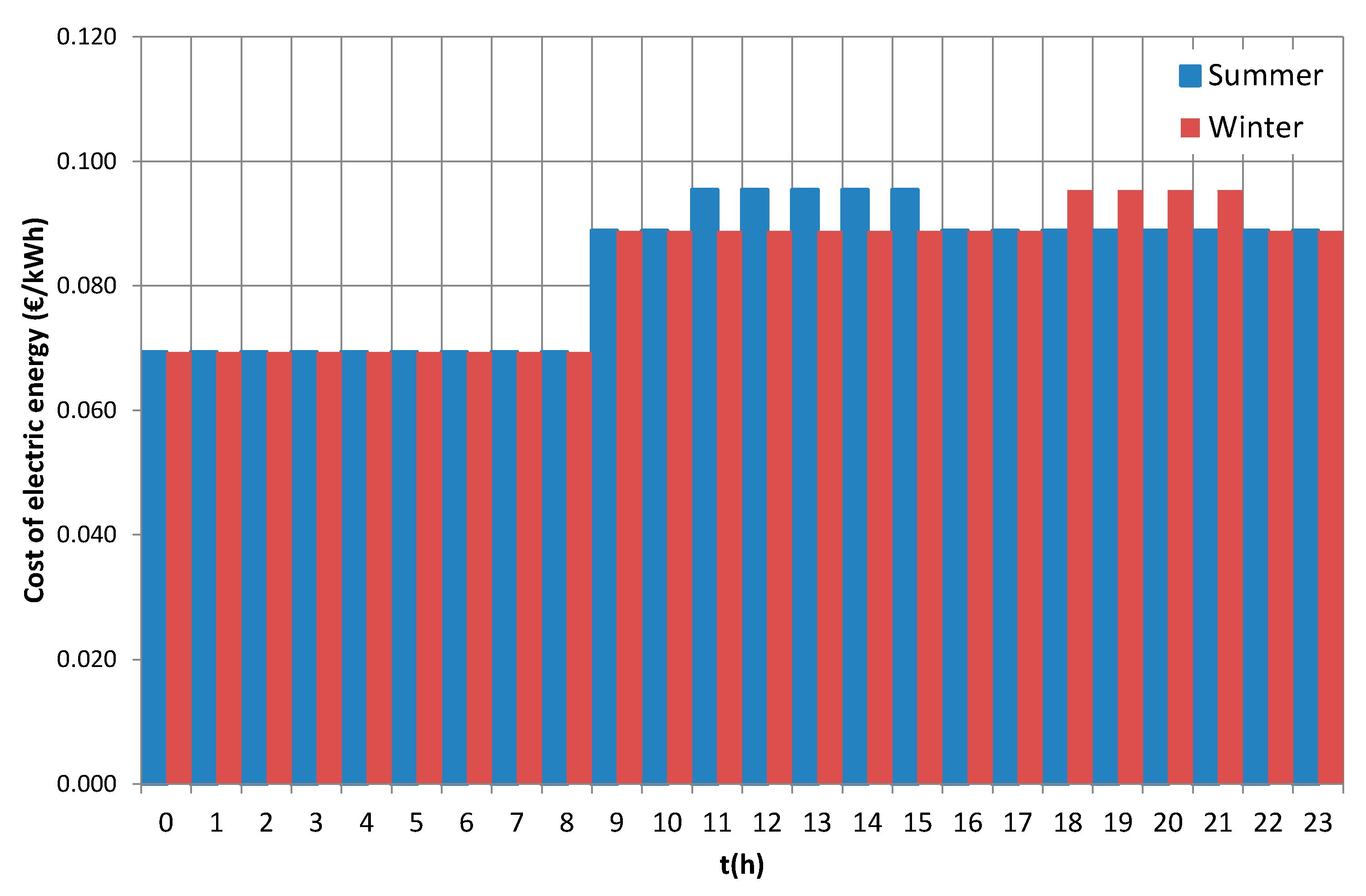
The electricity tariffs were obtained from the local electricity supply company (Endesa). As can be seen in
Figure 6, the tariffs vary in the summer and winter periods. It is assumed that there are 212 days corresponding to the summer period tariff and 153 to the winter period.
For the final design of the PS dimensions, the parameters of the PS basic design are: N1 = 20, N2 = 40, and N3 = 20. The design velocity of the PS pipes is Vmax = 2 m/s.
A database with 67 commercial centrifugal pump models is used. The details of this database are given in
Appendix A.
Each model was evaluated for this water supply system by varying the control modes and the number of FSP and VSP, whereby different combinations were obtained as alternatives. This process was developed through a calculation application, obtaining the following results:
The number of viable solutions was 65. These solutions correspond to pump models having the initial head H0 equal to or higher than the head corresponding to the maximum flow rate demanded H (Qmax). In this case study, the maximum flow is 44.1 l/s, and the maximum head required for this flow is 90.2 m. The viable solutions correspond to five models of pumps evaluated with different regulation modes, varying the number of FSPs and VSPs.
The process of analysing solutions to define the Pareto frontier reduces the number of alternatives to 43. These are the alternatives to which the AHP method is finally applied.
The application of the AHP method is based on the use of the global priority vectors of the factors and criteria defined in
Table 2. These priority vectors are used together with the ideal eigenvectors of the alternatives for each of the 43 dominant options.
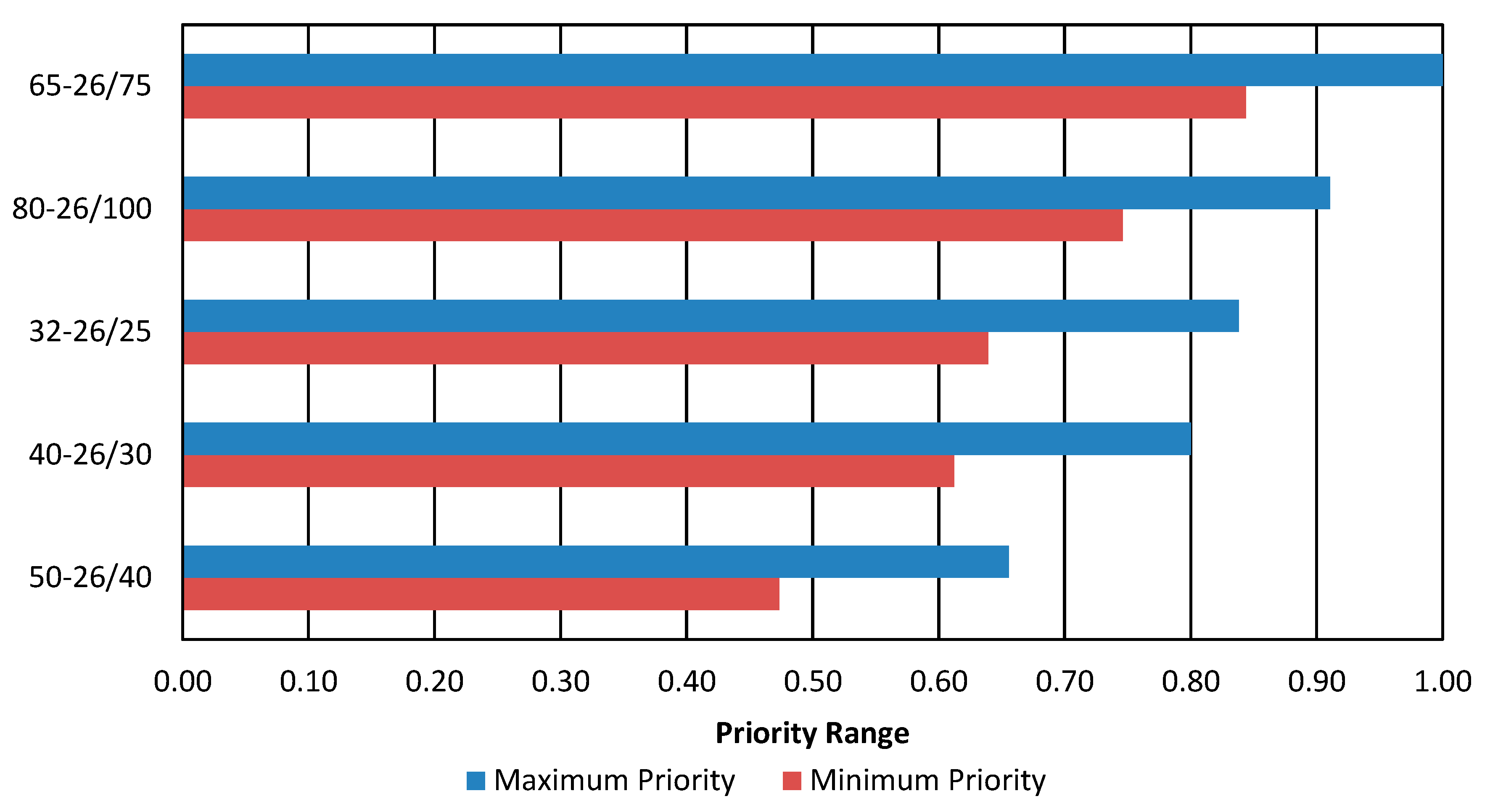
Figure 7 shows a summary of the results obtained from the application of the AHP method. It should be remembered that the 43 alternatives studied correspond to only five different pump models, but with different control schemes and different numbers of FSPs and VSPs. This is why
Figure 7 shows, for each model analysed, the range of prioritization of the best and the worst solutions.
In
Table 5, the values of the first solutions are presented, with top priority, which are hierarchical for each pump model. The criteria that are not reflected in
Table 5 are the same for all these alternatives. The full details of the values for each of the 43 alternatives are shown in the table of
Appendix B. In this table, the alternatives of each pump model that show a better prioritization after the application of the AHP method are highlighted in italics.
4. Discussion
The analysis of the values obtained for the 43 alternatives analysed and the final prioritization of the five models shown in
Table 5 provides some interesting insights. The first is that the best solutions with any pump model are obtained with the control model 4.2. In other words, the most appropriate control method for the PS for all models is based on achieving a head at the PS outlet equal to that of the setpoint curve for the flow rate supplied. This assumes all solutions have the same value in criterion C2 (PS control complexity) and criterion C6 (control system performance). In the case of criterion C2, the highest system complexity is obtained. On the other hand, the highest prioritization is obtained in criterion C6 since the control system performance is 100%. In short, according to the criteria defined by the experts, the additional investment cost of a 4.2 control system and its greater complexity are compensated by the advantages obtained in the better usage of the energy consumed.
Among the technical factors, flexibility is the criterion with the highest weight according to the assessment of the experts. Therefore, the greater the number of pumps, the higher the positive evaluation of this criterion. The alternative with the highest prioritization is the one with the highest number of pumps. This may influence the size of the PS, but criterion C1 has been defined with relatively low importance by the experts and consequently the size of the PS has almost no relevance in the final result.
Regarding the environmental factors, the experts’ assessment gives the MEI index a low relative weight. Despite this, the two pump models with the highest prioritizations have an MEI of 0.7, which guarantees the energy efficiency of the pump. On the contrary, the three alternatives with the lowest prioritizations have an MEI below 0.4, which is the minimum value established by the standard. This is because pump efficiency can have consequences on economic factors such as operating cost. A different aspect is the regulatory considerations. In the case of strictly applying a minimum MEI value of 0.4, only the first two models would be suitable and the three models with an MEI below 0.4 should be discarded and not considered as viable alternatives.
In the economic factors, the alternative with the best prioritization is not the cheapest in terms of investment costs. However, this alternative has the lowest operating costs. This criterion (C8, operation costs) was rated very highly (over 50%) by the experts among the economic factors. On the other hand, maintenance costs are slightly higher in the best rated solution compared to the other solutions. This is partly due to the higher number of elements (pumps, frequency inverters) than the other solutions. Criterion C9 related to PS maintenance was not highly rated by the experts. Thus, it seems that the increase in the number of pumps influences the investment and maintenance costs. However, the advantages derived from a better operation seem to economically compensate the higher investment and maintenance.
One of the features of the proposed method is the ability to generate different alternatives with the same pump model, but with different PS control schemes. These variations show the existence of different solutions for the same pump model. The best solutions appear for different control modes of the 65–26/75 model.
Figure 7 shows the priority ranking of each model evaluated in the AHP as viable alternatives. These ranges correspond to the priority of each model with different control modes and with different number of FSPs and VSPs.
Figure 7 shows for each model the solutions with the best and worst prioritization. Analysing in detail the results of
Figure 7 and the table of results in
Appendix B, it can be seen that the best rated alternatives are from the 65–26/75 model. Thus, several regulation modes with the 65–26/75 model have a higher prioritization than the best solution of the 80–26/100 model, which is the next in the hierarchical scale.
Once the AHP process has been developed, a sensitivity analysis is carried out varying the regulation equipment to be used. When making this change, the alternatives continue to be in the same hierarchical position, and the priority ranges of each of the models remain established in the same values, for which the distribution of the alternatives with respect to the optimum remains the same.
The objective of this work is not only to propose a new methodology. There are no bibliographic references with which to compare the proposed method, since a series of aspects are considered in a multicriteria decision that are not used in other types of designs. In this case, the comparison of the results are made with the result of applying the classic PS design methodology. Therefore, the same case study is solved below, but using a classical selection criterion.
In the traditional method, the number of pumps is selected arbitrarily. Sometimes it is based on the analysis of the variation of the demand pattern; in other cases, it is based on the experience of the designer. In any case, based on this number of pumps and the maximum flow rate of the PS, the flow rate to be supplied by the model to be selected is determined.
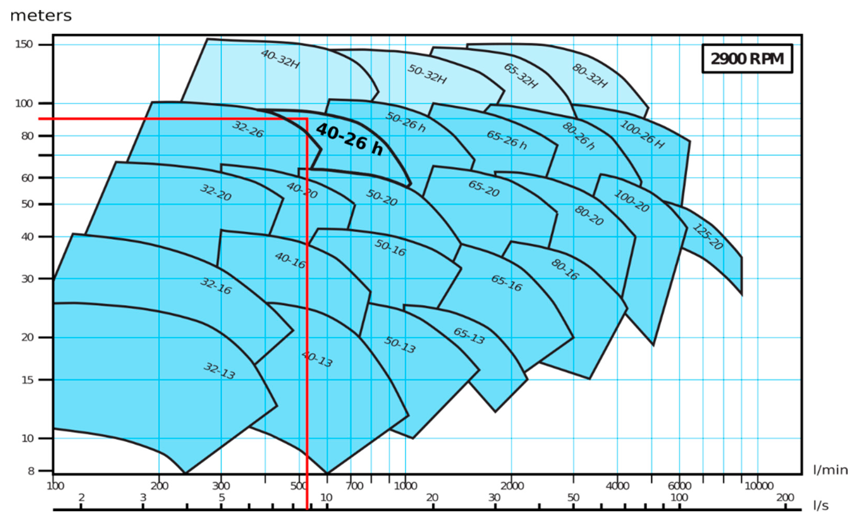
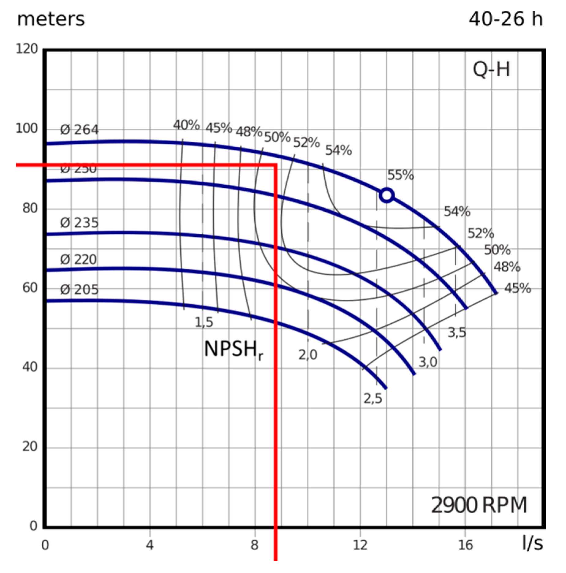
Consider for the case study analysed that a number of pumps equal to five is allowed. Taking into account that the maximum flow rate of the supply system is 44.1 l/s, the flow rate to be supplied by each pump will be 8.82 l/s. The head to be delivered by the pumps will be equal to that defined by the setpoint curve of the PS for the maximum flow. In this case this value is 90.2 m. These values of head and flow are used to select the required pump model in a catalogue as shown in
Figure 8.
According to
Figure 8, the group of pumps that is adjusted to the conditions of the supply system is 40–26 h.
Figure 9 shows the curves for these pumps and the location of the required pump point. Once the pump model is available, all possible regulation modes are evaluated. In this case the regulation modes are 1, 2.2, 3.1, 3.2, 4.1, and 4.2. The regulation mode 2.1 was not evaluated because it did not guarantee the overlap between switching the pumps on and off.
Table 6 shows the cost results of each of the alternatives with the different modes of regulation.
An analysis of the same type can be performed considering a different number of pumps in the PS.
Table 7 shows the result of applying the same methodology for a variable number of pumps between two and six. The result is different models of the database defined in
Appendix A.
To analyse these solutions, an annualized cost analysis has been performed: investment, operation, and maintenance. The annual operation and maintenance costs are available from the previous analysis (
Appendix B). The annual investment cost is obtained by annualizing the total investment costs of the PS.
The results of the operating economic analysis for the five models considered are given in
Table 8. In this table, for each model, the best control strategy (mode 4.2 in all cases) and the best combination of VSPs and FSPs have been selected. The table also shows the total investment, annual operation, and maintenance costs. Finally, it includes the total annualized cost after adding the annual amortization of the investment costs to the operation and maintenance costs.
As can be seen, the model that leads to the best results is 50–26/40. The results in the table are obtained for an amortization period of 10 years and an interest rate of 3%. A sensitivity analysis has been carried out on the amortization period (variations between 2 and 20 years) and the interest rate (between 0.5% and 8%), and in all cases the model that generates the lowest costs is the same.
Finally,
Table 9 compares the results obtained with the proposed methodology and the application of a traditional methodology. In the first case, the alternative with the highest prioritization has been selected. In the second case, the model that generates the lowest total annual cost is selected.
The analysis of
Table 9 concludes that the solution by the traditional method presents lower investment and maintenance costs but higher operating costs. Considering only the costs, the solution would be clear. However, the classical method does not take into account aspects such as the capacity of the PS to adapt to other flows (flexibility) or environmental aspects.
The lower operational costs of the solution by the proposed method (65–26/75) do not seem to economically compensate the excess investment required with respect to the classical solution (50–26/40). However, the model selected by the traditional method does not meet the constraints of the pump efficiency index (MEI): that is, it does not meet the minimum environmental requirements.
In the case of the methodology proposed in this work, according to the opinion of the experts surveyed, the use of a greater number of pumps (greater flexibility) or the use of higher efficiency pumps (better MEI index) can compensate for solutions that are apparently more costly from the economic point of view. In short, the final decision on the design of the PS should not only consider the economic evaluation of the solution but a multicriteria decision in which the AHP method can be of great help.
5. Conclusions
Traditional PS designs focus solely on economics. This design is based on the prior determination of its number of pumps. This decision is normally based on economic analysis, demand pattern analysis, or experience. However, determining the number of pumps in a PS has a direct consequence on its design, since many aspects are related to this number.
For this reason, a methodology that aims to improve the design process of a PS has been proposed. To do this, a basic design of the PS has been made, as indicated in
Figure 1. This basic design allows all the dimensions of the PS to be determined once the pump model is known. The method is based on using a database such as the one listed in
Appendix A. This database must have a wide range of heads and flow rates to be able to cover the operating range of the PS, defined by the setpoint curve and the demand pattern. The pump models in the database are verified to establish whether they are valid according to the defined design criteria. The number of PS design alternatives is high when considering the item number in the pump database. For each model, several control schemes of its operation are considered, as well as the different combinations of FSP and VSP. All of this generates the list of viable alternatives. This initial list of viable alternatives is reduced to those that form the Pareto frontier. The alternatives present in this border are the object of the application of the AHP method.
The AHP method is based on a series of experts giving their assessments of the weight of the different criteria. Subsequently, these same experts must assess the different alternatives with respect to the criteria. The main idea of the work is to simplify the participation of experts in this process. To do this, the process is broken down into two parts.
In the first part, once the factors and criteria have been defined, the experts only assess the weight of each one in determining the final solution. To weight the responses of the different experts, a geometric mean proportional to the inverse of their consistency index has been carried out. In this way, a global vector for the assessment of factors and criteria is obtained, as defined in
Table 2. This vector is general and can be applied in future PS projects.
The second part of applying the AHP method is the evaluation of the alternatives. This process has been automated since seven of the nine criteria can be quantitatively assessed. For the two qualitative criteria, a valuation rating has been defined by using a paired comparison matrix. The final result is a valuation method for each of the alternatives and a valuation vector for each criterion. Both elements allow ranking the different alternatives.
The weights obtained from the different decision criteria have a decisive influence on the classification of the alternatives. According to the experts’ responses, technical factors have a predominant aspect in the design of a PS. On the contrary, the economic aspects have a weight of 29%, a value much lower than that used in traditional design methodologies or in designs based on the LCC. Finally, environmental aspects have a weight of 22% in the final decision. Despite this relatively low weight, these environmental factors are the origin of the main differences between the proposed methodology and traditional approaches.
The number of viable alternatives on the Pareto frontier can be high: up to 43 in the case study. However, all these alternatives correspond to only five different pump models. From these five models the alternatives are generated considering the different control modes and the different numbers of FSPs and VSPs. There is a pump model (60–26/75) that has the highest priority hierarchy. That same model can work with different control schemes that still have a better hierarchy than the next model (80–26/100). However, not all 60–26/75 control schemes have better prioritization than the best 80–26/100 configuration. That is, the consideration of the PS control scheme is important in determining the final design solution.
In view of the results, it becomes clear that the use of the methodology allows other factors to be considered in the design process that classical methodologies do not consider. The economic valuation of the LCC is not enough to decide the design of a PS as defined in
Figure 1. Only an appropriate definition of all the factors that are part of the design of a PS and the valuation of the step of each of these factors can help in this process.
The method developed has a very large dependence on the result of the evaluation of the factors and criteria of the experts. To solve this, there are several options. One of them is to prepare this assessment each time the design process is carried out. The second is to expand the number of experts consulted and to have a global assessment vector that can be used in a wide typology of PSs.
The method developed is based on the parametric design of the PS in
Figure 1. The entire methodology was based on the quantitative assessment of the different alternatives that take said design as a reference. Additionally, the number of possible control schemes used is limited. Without a doubt, expanding the pump database, considering other PS schemes, or employing other PS control modes can enrich the design solutions obtained. In each case, the way of evaluating the alternatives may vary, or the number of alternatives may be different. However, in any case, the methodology presented can always be the basis upon which decisions are made.
Author Contributions
Conceptualization, C.X.B.-L., P.L.I.-R., F.J.M.-S.; Data curation, D.S.S.-F., C.X.B.-L.; Formal analysis, D.S.S.-F., C.X.B.-L., P.L.I.-R., F.J.M.-S.; Funding acquisition, P.L.I.-R., F.J.M.-S., V.S.F.-M.; Investigation, D.S.S.-F., C.X.B.-L., P.L.I.-R., F.J.M.-S., V.S.F.-M.; Methodology, D.S.S.-F., C.X.B.-L., P.L.I.-R., F.J.M.-S.; Project administration, P.L.I.-R., F.J.M.-S., V.S.F.-M.; Resources, P.L.I.-R., F.J.M.-S., V.S.F.-M.; Software, D.S.S.-F., C.X.B.-L., P.L.I.-R.; Supervision, P.L.I.-R., F.J.M.-S., V.S.F.-M.; Validation, D.S.S.-F., C.X.B.-L., P.L.I.-R.; Visualization, D.S.S.-F., C.X.B.-L., P.L.I.-R., F.J.M.-S.; Writing—original draft, D.S.S.-F., C.X.B.-L., P.L.I.-R., F.J.M.-S.; Writing—review & editing, P.L.I.-R., F.J.M.-S., V.S.F.-M. All authors have read and agreed to the published version of the manuscript.
Funding
This research received no external funding.
Institutional Review Board Statement
Not applicable.
Informed Consent Statement
Not applicable.
Data Availability Statement
Not applicable.
Conflicts of Interest
The authors declare no conflict of interest.
Appendix A
The BDD with which the case study has been developed is shown in
Table A1. This table contains 67 different models of a centrifugal pump manufacturer. The data collected for each pump model are:
Model number;
Model reference;
Nominal power (P) of the pump (kW);
Efficiency at BEP (Rmax);
Flow at BEP (Qopt) in l/s;
Head at BEL (Hopt) in m;
Maximum flow capacity of the pump (Qmax) in l/s. Characteristic parameters H0 and A of pump head curve: Hb = H0 − A·Q2;
Characteristic parameters E and F of the pump efficiency curve: η = E·Q − F·Q2.
Table A1.
Details of each pump model contained in the database.
Table A1.
Details of each pump model contained in the database.
| Model Number | Model Reference | P (kW) | Rmax | Qopt | Hopt | Qmax | H0 | A |
|---|
| 1 | 32–13/3 | 2.00 | 0.56 | 5.26 | 19.63 | 10.52 | 26.17 | 0.236 |
| 2 | 32–16/2 | 1.50 | 0.47 | 4.51 | 17.12 | 9.02 | 22.83 | 0.280 |
| 3 | 32–16/3 | 2.20 | 0.50 | 5.00 | 20.81 | 10.00 | 27.75 | 0.278 |
| 4 | 32–16/4 | 3.00 | 0.56 | 5.86 | 27.75 | 11.72 | 37.00 | 0.270 |
| 5 | 32–16/5.5 | 4.00 | 0.58 | 6.27 | 31.89 | 12.54 | 42.53 | 0.271 |
| 6 | 32–20/5.5 | 4.00 | 0.50 | 5.72 | 36.23 | 11.44 | 48.30 | 0.369 |
| 7 | 32–20/7.5 | 5.50 | 0.53 | 7.20 | 41.89 | 14.41 | 55.85 | 0.269 |
| 8 | 32–20/10 | 7.50 | 0.54 | 7.75 | 51.49 | 15.51 | 68.65 | 0.286 |
| 9 | 32–26/15 | 11.00 | 0.39 | 9.36 | 52.34 | 18.73 | 69.79 | 0.199 |
| 10 | 32–-26/20 | 15.00 | 0.43 | 9.65 | 69.26 | 19.29 | 92.35 | 0.248 |
| 11 | 32–26/25 | 18.50 | 0.45 | 10.59 | 77.06 | 21.18 | 102.75 | 0.229 |
| 12 | 40–13/5.5 | 4.00 | 0.78 | 12.57 | 20.19 | 25.14 | 26.92 | 0.043 |
| 13 | 40–16/4 | 3.00 | 0.53 | 8.52 | 20.99 | 17.04 | 27.99 | 0.096 |
| 14 | 40–16/5.5 | 4.00 | 0.63 | 10.58 | 25.39 | 21.17 | 33.86 | 0.076 |
| 15 | 40–16/7.5 | 5.50 | 0.66 | 12.34 | 31.94 | 24.68 | 42.59 | 0.070 |
| 16 | 40–20/7.5 | 5.50 | 0.56 | 7.79 | 31.00 | 15.59 | 41.33 | 0.170 |
| 17 | 40–20/10 | 7.50 | 0.59 | 10.68 | 42.39 | 21.37 | 56.51 | 0.124 |
| 18 | 40–20/15 | 11.00 | 0.61 | 12.14 | 50.80 | 24.27 | 67.73 | 0.115 |
| 19 | 40–26/15 | 11.00 | 0.49 | 11.74 | 44.48 | 23.49 | 59.30 | 0.107 |
| 20 | 40–26/20 | 15.00 | 0.53 | 12.70 | 56.41 | 25.40 | 75.21 | 0.117 |
| 21 | 40–26/30 | 22.00 | 0.55 | 15.09 | 75.35 | 30.18 | 100.47 | 0.110 |
| 22 | 50–13/3 | 2.20 | 0.73 | 14.93 | 11.83 | 29.86 | 15.77 | 0.018 |
| 23 | 50–13/4 | 3.00 | 0.74 | 16.52 | 14.35 | 33.03 | 19.13 | 0.018 |
| 24 | 50–13/5.5 | 4.00 | 0.76 | 21.43 | 17.61 | 42.86 | 23.49 | 0.013 |
| 25 | 50–13/7.5 | 5.50 | 0.76 | 21.94 | 20.45 | 43.87 | 27.26 | 0.014 |
| 26 | 50–16/7.5 | 5.50 | 0.74 | 18.77 | 22.06 | 37.55 | 29.42 | 0.021 |
| 27 | 50–16/10 | 7.50 | 0.76 | 21.32 | 28.56 | 42.64 | 38.08 | 0.021 |
| 28 | 50–16/15 | 11.00 | 0.77 | 24.25 | 32.72 | 48.50 | 43.63 | 0.019 |
| 29 | 50–20/15 | 11.00 | 0.68 | 17.39 | 41.61 | 34.78 | 55.49 | 0.046 |
| 30 | 50–20/20 | 15.00 | 0.70 | 19.47 | 47.65 | 38.94 | 63.54 | 0.042 |
| 31 | 50–20/25 | 18.50 | 0.70 | 19.35 | 50.43 | 38.70 | 67.24 | 0.045 |
| 32 | 50–26/30 | 22.00 | 0.61 | 22.71 | 61.06 | 45.42 | 81.41 | 0.039 |
| 33 | 50–26/40 | 30.00 | 0.63 | 24.32 | 78.73 | 48.63 | 104.98 | 0.044 |
| 34 | 65–13/7.5 | 5.50 | 0.70 | 4.71 | 15.38 | 9.42 | 20.50 | 0.231 |
| 35 | 65–13/10 | 7.50 | 0.73 | 5.30 | 17.13 | 10.59 | 22.83 | 0.203 |
| 36 | 65–13/15 | 10.00 | 0.76 | 5.99 | 20.11 | 11.99 | 26.81 | 0.187 |
| 37 | 65–16/15 | 11.00 | 0.76 | 5.66 | 25.02 | 11.32 | 33.36 | 0.261 |
| 38 | 65–16/20 | 15.00 | 0.81 | 6.50 | 33.33 | 12.99 | 44.44 | 0.263 |
| 39 | 65–20/20 | 15.00 | 0.72 | 6.09 | 30.97 | 12.17 | 41.29 | 0.279 |
| 40 | 65–20/25 | 18.50 | 0.74 | 7.14 | 36.85 | 14.27 | 49.14 | 0.241 |
| 41 | 65–20/30 | 22.00 | 0.75 | 7.07 | 41.27 | 14.13 | 55.03 | 0.275 |
| 42 | 65–20/40 | 30.00 | 0.77 | 7.99 | 51.69 | 15.97 | 68.92 | 0.270 |
| 43 | 65–26/50 | 37.00 | 0.73 | 8.08 | 62.06 | 16.16 | 82.74 | 0.317 |
| 44 | 65–26/60 | 45.00 | 0.75 | 8.71 | 70.09 | 17.41 | 93.45 | 0.308 |
| 45 | 65–26/75 | 55.00 | 0.77 | 9.06 | 78.19 | 18.11 | 104.25 | 0.318 |
| 46 | 80–16/15 | 11.00 | 0.75 | 8.31 | 19.93 | 16.61 | 26.58 | 0.096 |
| 47 | 80–16/20 | 15.00 | 0.78 | 8.29 | 24.87 | 16.57 | 33.16 | 0.121 |
| 48 | 80–16/25 | 18.50 | 0.82 | 10.24 | 26.12 | 20.48 | 34.83 | 0.083 |
| 49 | 80–16/30 | 22.00 | 0.84 | 10.98 | 29.71 | 21.96 | 39.62 | 0.082 |
| 50 | 80–20/30 | 22.00 | 0.78 | 9.40 | 36.79 | 18.79 | 49.06 | 0.139 |
| 51 | 80–20/40 | 30.00 | 0.79 | 10.53 | 40.64 | 21.06 | 54.18 | 0.122 |
| 52 | 80–20/50 | 37.00 | 0.80 | 11.92 | 44.71 | 23.83 | 59.61 | 0.105 |
| 53 | 80–20/60 | 45.00 | 0.81 | 12.69 | 49.27 | 25.38 | 65.69 | 0.102 |
| 54 | 80–26/60 | 45.00 | 0.82 | 9.82 | 55.09 | 19.63 | 73.46 | 0.191 |
| 55 | 80–26/75 | 55.00 | 0.82 | 12.39 | 64.58 | 24.78 | 86.11 | 0.140 |
| 56 | 80–26/100 | 75.00 | 0.80 | 13.41 | 75.73 | 26.83 | 100.97 | 0.140 |
| 57 | 100–20/30 | 22.00 | 0.78 | 11.78 | 31.18 | 23.57 | 41.57 | 0.075 |
| 58 | 100–20/40 | 30.00 | 0.81 | 14.00 | 36.14 | 28.01 | 48.18 | 0.061 |
| 59 | 100–20/50 | 37.00 | 0.82 | 14.96 | 40.28 | 29.91 | 53.70 | 0.060 |
| 60 | 100–20/60 | 45.00 | 0.83 | 16.64 | 44.99 | 33.28 | 59.98 | 0.054 |
| 61 | 100–20/75 | 55.00 | 0.83 | 19.16 | 48.81 | 38.31 | 65.09 | 0.044 |
| 62 | 100–26/60 | 45.00 | 0.83 | 12.53 | 47.06 | 25.05 | 62.74 | 0.100 |
| 63 | 100–26/75 | 55.00 | 0.83 | 14.86 | 53.77 | 29.72 | 71.69 | 0.081 |
| 64 | 100–26/100 | 75.00 | 0.83 | 16.97 | 61.52 | 33.94 | 82.03 | 0.071 |
| 65 | 125–20/60 | 45.00 | 0.70 | 25.37 | 33.41 | 50.74 | 44.54 | 0.017 |
| 66 | 125–20/75 | 55.00 | 0.72 | 25.23 | 37.03 | 50.45 | 49.37 | 0.019 |
| 67 | 125–20/100 | 75.00 | 0.74 | 24.13 | 40.93 | 48.27 | 54.58 | 0.023 |
Appendix B
The application of the proposed methodology to the case study generates 65 different alternatives. The calculation of the Pareto frontier with the dominant solutions reduces the number of study alternatives to 43. The following table shows the valuation details of each of these alternatives. The following information is collected for each one:
Sol: Solution/Alternative number;
Mod: Number of the selected pump model, according to the database in
Appendix A;
Nb: Number of pumps installed in the PS;
N: VSP number of the PS;
m: FSP number of the PS;
C1: PS size (m2);
C2: Complexity or control mode of the PS;
C3: Flexibility (number of pumps);
C4: MEI: pump energy efficiency index (energy efficiency index of the pump);
C5: CO2 emissions (kg/year);
C6: Control system performance;
C7: Investments costs (€/year);
C8: Operation costs (€/year);
C9: Maintenance costs (€/year).
Table A2.
Details of each solution and its valuation according to each factor and criterion.
Table A2.
Details of each solution and its valuation according to each factor and criterion.
| Sol | Mod | Nb | n | m | C1 | C2 | C3 | C4 | C5 | C6 | C7 | C8 | C9 |
|---|
| 1 | 11 | 6 | 0 | 6 | 144 | 1 | 6 | 0.10 | 1,624,452.55 | 0.61 | 67,989.68 | 61,101.73 | 1823.27 |
| 2 | 11 | 6 | 0 | 6 | 144 | 2.2. | 6 | 0.10 | 403,218.18 | 0.75 | 69,768.00 | 29,562.30 | 1918.87 |
| 3 | 11 | 6 | 1 | 5 | 144 | 4.1. | 6 | 0.10 | 753,838.06 | 0.64 | 71,009.71 | 39,564.78 | 1902.53 |
| 4 | 11 | 6 | 1 | 5 | 144 | 4.2. | 6 | 0.10 | 362,746.21 | 1.00 | 72,508.39 | 24,512.03 | 1960.80 |
| 5 | 11 | 6 | 2 | 4 | 144 | 4.2. | 6 | 0.10 | 349,937.99 | 1.00 | 74,617.58 | 23,284.44 | 1983.23 |
| 6 | 11 | 6 | 3 | 3 | 144 | 4.2. | 6 | 0.10 | 347,737.86 | 1.00 | 76,726.77 | 23,142.73 | 2005.66 |
| 7 | 11 | 6 | 4 | 2 | 144 | 4.2. | 6 | 0.10 | 346,894.78 | 1.00 | 78,835.96 | 23,094.27 | 2028.09 |
| 8 | 11 | 6 | 5 | 1 | 144 | 4.2. | 6 | 0.10 | 346,894.42 | 1.00 | 80,945.15 | 23,094.25 | 2050.51 |
| 9 | 11 | 6 | 6 | 0 | 144 | 3.2. | 6 | 0.10 | 346,894.19 | 1.00 | 83,054.34 | 23,094.24 | 2072.94 |
| 10 | 21 | 5 | 0 | 5 | 130 | 1 | 5 | 0.10 | 1,255,991.15 | 0.61 | 63,175.81 | 56,644.95 | 1547.31 |
| 11 | 21 | 5 | 0 | 5 | 130 | 2.2. | 5 | 0.10 | 292,152.93 | 0.71 | 64,954.13 | 26,539.60 | 1642.91 |
| 12 | 21 | 5 | 1 | 4 | 130 | 4.1. | 5 | 0.10 | 480,084.71 | 0.64 | 66,516.60 | 33,674.23 | 1626.57 |
| 13 | 21 | 5 | 1 | 4 | 130 | 4.2. | 5 | 0.10 | 250,885.17 | 1.00 | 68,015.28 | 20,556.95 | 1684.83 |
| 14 | 21 | 5 | 2 | 3 | 130 | 4.2. | 5 | 0.10 | 236,786.70 | 1.00 | 70,445.23 | 19,026.69 | 1707.26 |
| 15 | 21 | 5 | 3 | 2 | 130 | 4.2. | 5 | 0.10 | 235,658.64 | 1.00 | 72,875.18 | 18,943.78 | 1729.69 |
| 16 | 21 | 5 | 4 | 1 | 130 | 4.2. | 5 | 0.10 | 235,589.75 | 1.00 | 75,305.14 | 18,940.33 | 1752.12 |
| 17 | 21 | 5 | 5 | 0 | 130 | 3.2. | 5 | 0.10 | 235,548.00 | 1.00 | 77,735.09 | 18,938.23 | 1774.55 |
| 18 | 33 | 3 | 0 | 3 | 123 | 1 | 3 | 0.10 | 667,553.08 | 0.58 | 51,875.30 | 50,185.13 | 1002.24 |
| 19 | 33 | 3 | 0 | 3 | 123 | 2.1. | 3 | 0.10 | 288,570.67 | 0.61 | 52,322.15 | 33,407.16 | 1014.38 |
| 20 | 33 | 3 | 0 | 3 | 123 | 2.2. | 3 | 0.10 | 196,483.83 | 0.64 | 53,653.62 | 27,160.20 | 1097.85 |
| 21 | 33 | 3 | 1 | 2 | 123 | 4.1. | 3 | 0.10 | 280,108.70 | 0.64 | 55,893.76 | 30,523.68 | 1081.51 |
| 22 | 33 | 3 | 1 | 2 | 123 | 4.2. | 3 | 0.10 | 143,536.87 | 1.00 | 57,392.44 | 17,408.26 | 1139.77 |
| 23 | 33 | 3 | 2 | 1 | 123 | 4.2. | 3 | 0.10 | 135,114.96 | 1.00 | 60,500.06 | 16,423.45 | 1162.20 |
| 24 | 33 | 3 | 3 | 0 | 123 | 3.2. | 3 | 0.10 | 134,789.20 | 1.00 | 63,607.68 | 16,396.20 | 1184.63 |
| 25 | 45 | 7 | 0 | 7 | 158 | 1 | 7 | 0.70 | 1,121,560.31 | 0.60 | 117,481.59 | 36,159.93 | 2099.23 |
| 26 | 45 | 7 | 0 | 7 | 158 | 2.2. | 7 | 0.70 | 257,719.92 | 0.77 | 119,259.91 | 17,050.84 | 2194.84 |
| 27 | 45 | 7 | 1 | 6 | 158 | 4.1. | 7 | 0.70 | 430,332.72 | 0.64 | 123,120.04 | 21,560.97 | 2178.50 |
| 28 | 45 | 7 | 1 | 6 | 158 | 4.2. | 7 | 0.70 | 235,340.18 | 1.00 | 124,618.71 | 14,473.14 | 2236.76 |
| 29 | 45 | 7 | 2 | 5 | 158 | 4.2. | 7 | 0.70 | 225,639.11 | 1.00 | 129,346.32 | 13,516.62 | 2259.19 |
| 30 | 45 | 7 | 3 | 4 | 158 | 4.2. | 7 | 0.70 | 224,695.74 | 1.00 | 134,073.93 | 13,460.00 | 2281.62 |
| 31 | 45 | 7 | 4 | 3 | 158 | 4.2. | 7 | 0.70 | 224,592.64 | 1.00 | 138,801.53 | 13,455.04 | 2304.05 |
| 32 | 45 | 7 | 5 | 2 | 158 | 4.2. | 7 | 0.70 | 224,565.74 | 1.00 | 143,529.14 | 13,454.07 | 2326.48 |
| 33 | 45 | 7 | 6 | 1 | 158 | 4.2. | 7 | 0.70 | 224,547.70 | 1.00 | 148,256.75 | 13,453.42 | 2348.91 |
| 34 | 45 | 7 | 7 | 0 | 158 | 3.2. | 7 | 0.70 | 224,534.77 | 1.00 | 152,984.36 | 13,452.96 | 2371.34 |
| 35 | 56 | 6 | 0 | 6 | 144 | 1 | 6 | 0.70 | 1,101,911.25 | 0.60 | 140,018.56 | 41,401.73 | 1823.27 |
| 36 | 56 | 6 | 0 | 6 | 144 | 2.2. | 6 | 0.70 | 218,101.86 | 0.73 | 141,796.88 | 17,718.71 | 1918.87 |
| 37 | 56 | 6 | 1 | 5 | 144 | 4.1. | 6 | 0.70 | 379,675.78 | 0.64 | 146,410.03 | 23,052.97 | 1902.53 |
| 38 | 56 | 6 | 1 | 5 | 144 | 4.2. | 6 | 0.70 | 192,692.03 | 1.00 | 147,908.70 | 14,143.77 | 1960.80 |
| 39 | 56 | 6 | 2 | 4 | 144 | 4.2. | 6 | 0.70 | 183,970.44 | 1.00 | 153,389.33 | 13,227.15 | 1983.23 |
| 40 | 56 | 6 | 3 | 3 | 144 | 4.2. | 6 | 0.70 | 183,251.79 | 1.00 | 158,869.96 | 13,189.42 | 2005.66 |
| 41 | 56 | 6 | 4 | 2 | 144 | 4.2. | 6 | 0.70 | 182,990.78 | 1.00 | 164,350.58 | 13,178.50 | 2028.09 |
| 42 | 56 | 6 | 5 | 1 | 144 | 4.2. | 6 | 0.70 | 182,830.34 | 1.00 | 169,831.21 | 13,171.79 | 2050.51 |
| 43 | 56 | 6 | 6 | 0 | 144 | 3.2. | 6 | 0.70 | 182,721.76 | 1.00 | 175,311.84 | 13,167.25 | 2072.94 |
References
- United Nations; UN WATER. Development Report 2020: Water and Climate Change; United Nations: París, France, 2020. [Google Scholar]
- Pelli, T.; Hitz, H. Energy indicators and savings in water supply. J. Am. Water Work. Assoc. 2000, 92, 55–62. [Google Scholar] [CrossRef]
- Pasha, M.F.; Lansey, K. Optimimal Pump Scheduling by linear programming. World Environ. Water Resour. 2009, 1–10. [Google Scholar] [CrossRef]
- Sakarya, A.B.A.; Mays, L.W. Optimal Operation of Water Distribution Pumps Considering Water Quality. J. Water Resour. Plan. Manag. 2000, 126, 210–220. [Google Scholar] [CrossRef]
- Ibarra, D.; Arnal, J. Parallel Programming Techniques Applied to Water Pump Scheduling Problems. J. Water Resour. Plan. Manag. 2014, 140, 06014002. [Google Scholar] [CrossRef]
- López-Ibáñez, M.; Prasad, T.D.; Paechter, B. Ant Colony Optimization for Optimal Control of Pumps in Water Distribution Networks. J. Water Resour. Plan. Manag. 2008, 134, 337–346. [Google Scholar] [CrossRef]
- Giacomello, C.; Kapelan, Z.; Nicolini, M. Fast Hybrid Optimization Method for Effective Pump Scheduling. J. Water Resour. Plan. Manag. 2013, 139, 175–183. [Google Scholar] [CrossRef]
- Yu, G.; Powel, R.; Sterling, M. Optimized Pump Scheduling in water distribution systems. J. Optim. Theory Appl. 1994, 83, 463–488. [Google Scholar] [CrossRef]
- Wu, W.; Gao, J. Enhancing the Reliability and Security of Urban Water Infrastructures through Intelligent Monitoring, Assessment, and Optimization. Intell. Infrastruct. 2009, 487–516. [Google Scholar] [CrossRef]
- Chang, Y.; Choi, G.; Kim, J.; Byeon, S. Energy cost optimization for water distribution networks using demand pattern and storage facilities. Sustainability 2018, 10, 1118. [Google Scholar] [CrossRef] [Green Version]
- Lipiwattanakarn, S.; Kaewsang, S.; Charuwimolkul, N.; Changklom, J.; Pornprommin, A. Theoretical Estimation of Energy Balance Components in Water Networks for Top-Down Approach. Water 2021, 13, 1011. [Google Scholar] [CrossRef]
- Giudicianni, C.; Herrera, M.; di Nardo, A.; Carravetta, A.; Ramos, H.M.; Adeyeye, K. Zero-net energy management for the monitoring and control of dynamically-partitioned smart water systems. J. Clean. Prod. 2020, 252, 119745. [Google Scholar] [CrossRef]
- Martin-Candilejo, A.; Santillán, D.; Iglesias, A.; Garrote, L. Optimization of the Design of Water Distribution Systems for Variable Pumping Flow Rates. Water 2020, 12, 359. [Google Scholar] [CrossRef] [Green Version]
- Briceño-León, C.X.; Iglesias-Rey, P.L.; Martinez-Solano, F.J.; Mora-Melia, D. Use of Fixed and Variable Speed Pumps in Water Distribution Networks with Different Control Strategies. Water 2021, 479, 23. [Google Scholar]
- Nault, J.; Papa, F. Lifecycle Assessment of a Water Distribution System Pump. J. Water Resour. Plan. Manag. 2015, 141, 1–9. [Google Scholar] [CrossRef]
- Ossadnik, W.; Schinke, S.; Kaspar, R.H. Group Aggregation Techniques for Analytic Hierarchy Process and Analytic Network Process: A Comparative Analysis. Group Decis. Negot. 2016, 25, 421–457. [Google Scholar] [CrossRef] [Green Version]
- Saaty, T. The analytic hierarchy process (AHP). J. Oper. Rese. Soc. 1980, 41, 1073–1076. [Google Scholar]
- Saaty, T.L. Decision making with the analytic hierarchy process. Int. J. Serv. Sci. 2008, 1, 83. [Google Scholar] [CrossRef] [Green Version]
- Saaty, T.L. Rank from comparisons and from ratings in the analytic hierarchy/network processes. Eur. J. Oper. Res. 2006, 168, 557–570. [Google Scholar] [CrossRef]
- Shapira, A.; Goldenberg, M. AHP-Based Equipment Selection Model for Construction Projects. J. Constr. Eng. Manag. 2005, 131, 1263–1273. [Google Scholar] [CrossRef]
- Kurbatova, A.; Abu-Qdais, H.A. Using multi-criteria decision analysis to select waste to energy technology for a Mega city: The case of Moscow. Sustainability 2020, 12, 9828. [Google Scholar] [CrossRef]
- Medland, S.; Shaker, R.; Forsythe, K.; Mackay, B.; Rybarczyk, G. A multi-Criteria Wetland Suitability Index for Restoration across Ontario’s Mixedwood Plains. Sustainability 2020, 12, 9953. [Google Scholar] [CrossRef]
- Du, C. Dynamic evaluation of sustainable water resource systems in metropolitan areas: A case study of the beijing megacity. Water 2020, 12, 2629. [Google Scholar] [CrossRef]
- Leon-Celi, C.; Iglesias-Rey, P.L.; Martinez Solano, F.J.; Mora-Meliá, D. A methodology for the optimization of flow rate injection to looped water distribution networks through multiple pumping stations. Water 2016, 8, 575. [Google Scholar] [CrossRef] [Green Version]
- Iglesias Rey, P.L.; Martínez Solano, F.J.; Arango Gil, F.; Lozano Cortés, J. Methodology for the selection of pumping stations considering its mode of operation. In Proceedings of the 10th International Perspectives on Water Resources and the Environment (IPWE), Cartagena, Columbia, 3–7 December 2018. [Google Scholar]
- Abbass, H.; Sarker, R.; Newton, C. A Pareto-frontier differential evolution approach for multi-objective optimization problems. In Proceedings of the 2001 Congress on Evolutionary Computation, Seoul, Korea, 27–30 May 2001; Volume 2, pp. 971–978. [Google Scholar]
- European Union Comission Regularion No 547/2012. Implementing Directive 2009/125/EC of the Eoperan Parliament and of the Council with Regard to Ecodesign Requierements for Water Pumps. Official Journal of the European Union, 25 June 2012.
| Publisher’s Note: MDPI stays neutral with regard to jurisdictional claims in published maps and institutional affiliations. |
© 2021 by the authors. Licensee MDPI, Basel, Switzerland. This article is an open access article distributed under the terms and conditions of the Creative Commons Attribution (CC BY) license (https://creativecommons.org/licenses/by/4.0/).


 ,
, 


