Article

Multivariate Modeling of Mechanical Properties for Hot Runner Molded Bioplastics and a Recycled Polypropylene Blend

1
Department of Plastics Engineering, University of Massachusetts Lowell, Lowell, MA 01854, USA
2
Department of Mechanical Engineering, Università Degli Studi Di Padova, 2-35122 Padova, Italy
3
Department of Materials Science, University of Oxford, Oxford OX1 2JD, UK
4
Mold-Masters Ltd., Georgetown, ON L7G 4X5, Canada
*
Author to whom correspondence should be addressed.
Sustainability 2021, 13(14), 8102; https://0-doi-org.brum.beds.ac.uk/10.3390/su13148102
Submission received: 8 June 2021 / Revised: 9 July 2021 / Accepted: 15 July 2021 / Published: 20 July 2021
(This article belongs to the Special Issue Intelligent Sensing for Sustainable Production Industries)

Abstract

:
Four sustainable materials including a recycled polypropylene blend, polybutylene adipate terephthalate, and two grades of polylactic acid are compared to a reference isotactic polypropylene. Tensile specimens were produced using a two-cavity, hot runner mold with fully automatic cycles per standard industrial practices to investigate the effect of melt temperature, injection velocity, cycle time, and screw speed on the mechanical properties. Multiple regression and principal component analyses were performed for each of the materials. Results indicated that all the materials were readily processed using a hot runner, and the mechanical properties exhibited minimal variation. To the extent that losses in mechanical properties were observed, the results indicated that the losses were correlated with thermal degradation as independently characterized by thermal gravimetric analysis. Such losses can be minimized by reducing melt temperature and cycle time, leading to a reduction of the environmental impact of injection molding processes.

1. Introduction

Increasing environmental concerns require a formal analysis of sustainability at the product design phase to assure appropriate material selection and use [1]. Many firms seek to support a circular economy [2] in which the industrial economy is regenerative by design. A literature review [3] of eco-design indicated that the most common best practices included post-use recycling (98%) and pre-use eco-design (93%), followed by design for re-use (93%), repair (44%), durability (35%), refurbishing (30%), disassembly (26%), remanufacture (23%), and repurpose (2%).
There are several performance metrics for eco-design [4], with two of the most common being “embodied energy” and “carbon footprint”. Ashby [5] defined embodied energy as the energy consumed to produce 1 kg of material. By comparison, carbon footprint represents the total direct and indirect CO2 given a product, process, or activity over its entire lifetime [6]. While energy consumption during product use is a significant concern in the transportation industries, Rydh et al. [7] found that the emission of carbon dioxide in product design and manufacturing is practically linear with the embodied energy of the consumed materials; the same correlation between embodied energy and carbon footprint was also evident in many of the case studies described by Morini et al. [4].
Designers and manufacturers of plastic products can maximize sustainability by (1) selecting materials to minimize the embodied energy of their products, and (2) designing their products for recycling. For example, bioplastics such as polylactic acid (PLA) and poly(3-hydroxybutyrate-co-3-hydroxyvalerate) (PHBV) may have low environmental impact compared to traditional thermoplastics [8,9,10]. At the same time, the use of recycled resins and especially blends of polyethylene (PE) and polypropylene (PP) are of great interest [11,12,13]. However, both bioplastics and recycled blends are sometimes considered low-performance materials with respect to their mechanical properties. Specifically, many bioplastics have inferior brittleness, thermal stability, melt strength, processing robustness, and other structural properties compared to traditional thermoplastics [14]. Meanwhile, mechanical properties of recyclates are also of potential concern due to the additional heat cycle(s) in processing and sensitivity to possible contamination [15].
This article investigates the process:property relations of different commercially available bioplastics and a recycled PE/PP blend in a pilot production environment using an instrumented two-cavity, hot runner injection mold. The process settings are set according to ordinary molding practices, typical of a plastics manufacturer using commodity polypropylene. As described, a design of experiments is implemented to test the robustness of the candidate materials across a wide range of operating conditions to specifically investigate the robustness of the material with respect to processing temperatures, residence times, and shear rates. The mechanical properties of the molded samples are tested, and a set of principal component analyses are performed to characterize the process:property relations. Propagation of variance is then applied to estimate the expected range of mechanical properties in the commercial use of the sustainable plastics. The results are highly encouraging insomuch as they indicate that the bioplastic and recycled materials are viable alternatives to the reference polypropylene.

2. Materials and Methods

2.1. Materials Selection and Overview

As summarized in Table 1, the investigated materials were selected to approximate a reference commodity material, Pro-fax PD702 (LyondellBasell, Houston, TX, USA). This reference material is an isotactic polypropylene (referred to as iPP) homopolymer with a melt flow rate of 35 g/10 min per ASTM D1238, which is typically used in injection molding of consumer products, packaging, and other applications. The alternates included a recycled polypropylene/polyethylene (referred to as rPP), a biodegradable polyester (polybutylene adipate terephthalate, PBAT), and two polylactic acid polymers supplied by NatureWorks and Vegeplast (respectively referred to as PLA-N and PLA-V). The suppliers and grades were provided with recommended melt temperatures and the representative melt flow rates and mechanical properties.
Inspection of the data in Table 1 suggests that the materials are quite similar with respect to their processing conditions. The mechanical properties of the iPP and rPP are also quite similar, though all the bioplastics tend to exhibit higher tensile modulus and more brittle behavior. The thermal history of a specimen affects the initial yielding behavior of the thermoplastic materials, but not the plastic flow in the post-yield regime. For the post-yield regime, the deformation rate and temperature are relevant control parameters for the stress.

2.2. Mold Design and Processing Methodology

A two-cavity hot runner mold was supplied by Milacron Mold-Masters (Georgetown, ON, Canada) and used to injection mold ASTM tensile bars having a nominal thickness of 3.18 mm, gage length of 75 mm, and gage width of 12.7 mm. Hot runner molds maintain the plastic in the feed system in a molten state. Hot runner molds have significant potential advantages with respect to sustainability because they (1) avoid the material waste associated with molding of the runners and (2) allow for cycle time improvement on the order of 100% compared to cold runner molds, since they do not need to plasticate or cool material in the feed system [16]. However, the use of hot runner molds introduces longer residence times of the material at elevated temperatures, given the additional melt volume in the feed system. These longer residence times are potentially detrimental to bioplastics that are known to be more susceptible to thermal degradation [17].
The layout design of the hot runner mold is shown in Figure 1, with the two tensile specimen cavities indicated in red. The hot runner mold connects the nozzle of the molding machine to the mold cavities via a heated sprue. The sprue connects to the center of a straight manifold that then directs the melt to hot runner nozzles that connect to a gate in each of the two cavities located in the grip section of the tensile specimens. Given potential degradation concerns, the volume of the melt in the feed system was estimated as three times the volume of the cavities based on visual inspection during material and accompanying color changes. Approximately ten cycles were estimated to be required to change the bulk of the material in the feed system, and 30 molding cycles were performed prior to acceptance of specimens at start-up and between material changes.
The effect of processing conditions on potential material property degradation was investigated by varying parameters that directly affect the melt temperature (i.e., hot runner temperature and plastication speed) and those that affect the residence time (i.e., injection velocity and cooling time). The hot runner temperature, plastication speed, and cooling time were each specified with two levels, while the injection velocity was specified with four levels as reported in Table 2. A full factorial design of experiments (DOE) was implemented wherein the resulting DOE had 2 × 2 × 2 × 4 or 32 runs as specified in Table A1. The DOE was repeated for each of the five materials with the same processing parameters except for the hot runner and barrel temperatures. Specifically, the hot runner/barrel temperature was purposefully set to a broader range for iPP (between 180 and 220 °C) to investigate possible degradation at higher temperatures. Otherwise, the hot runner and barrel temperatures were set at 180 and 200 °C per material supplier recommendations. The molding was operated in fully automatic mode with other process parameters held constant, including a mold coolant temperature of 40 °C, packing pressure of 15 MPa, a packing time of 8 s, and a mold open time of 5 s.
To minimize sources of external variability, polymers were taken from single batches. Resins were pre-dried before molding at 170 °C for 4 h and then directly transferred into the molding machine using a sealed hopper. To avoid resin contamination, PP was purged through at process start-up and shut down, with 60 automatic molding cycles performed and the resulting moldings discarded at every production start-up. To guarantee stability of the molding process and of the data acquisition setup, 30 molding cycles were discarded for each DOE run before collecting the first part. Then 30 parts were collected for each DOE run on a fully automatic cycle with no interruptions. The response variables considered in the later analysis included the melt temperature (measured via an intrusive thermocouple located in the nozzle), the cycle time, and the temperature of the molded parts (measured immediately after ejection).
Parts were visually inspected, labeled, and stored for later structural characterization. The mechanical properties of the molded parts were characterized by means of tensile testing at room temperature (conditioned at 21 °C) according to ASTM D638. The thickness of the tensile specimens was measured with a micrometer and entered to evaluate the applied stresses. The tests were carried out with a speed of 10 mm/min using an Instron Universal Testing Machine (Norwood, MA, USA). For each DOE run, molded parts for each cavity were selected for cycles 10, 20, and 30 and were characterized, resulting in a total of 192 tests for each resin. Elastic modulus, stress at break, and strain at break were evaluated from the observed stress–strain behavior for comparison of the mechanical properties of the different resins and the effect of hot runner molding. A data color spectrophotometer (Datacolor DC500, Lucerne, Switzerland) was also used to evaluate the effect of degradation on the color shift and visual appearance of the molded parts.

2.3. Biopolymer Properties

The rheological properties of the five investigated materials were characterized with a capillary rheometer (Dynisco LCR 7600, Franklin, MA, USA) with a capillary die having a bore diameter of 1 mm and bore length of 30 mm. The apparent viscosity of the materials at temperatures of 180 and 200 °C are plotted in Figure 2. It was observed that all five materials had relatively similar shear-thinning behaviors with a viscosity on the order of 100 Pa*s at a shear rate of 1000 s−1, which was representative of the shear rates in the mold cavity at a flow rate of 32 mL/s (near the mid-point of the injection velocities as indicated in Table 2). The iPP and rPP tended to have the lowest viscosities, while the PBAT and PLA-V had the greatest temperature sensitivity. The PLA-N had the highest viscosities. Regardless, all five of the investigated materials were readily processed at the DOE run settings without difficulty.
Differential scanning calorimetry (DSC) was performed to evaluate the onset of melting and specific heat with a heat–cool–heat cycle, heating rate of 10 °C/min, from 50 to 200 °C. The results for the onset of melting are reported in the fifth row of Table 1 for the five investigated materials; the iPP and rPP melted around 155 °C while the bioplastics varied from 144 °C for the PLA-V to 163 °C for the PBAT and PLA-N.
The thermal degradation properties of the five investigated materials were characterized via thermal gravimetric analysis (TA Instruments TGA 2950, Wakefield, MA, USA) at a heating ramp rate of 10 °C/min in a nitrogen environment. The results are plotted in Figure 3 with the observed peak degradation temperatures reported in the sixth row of Table 1. The results suggested that all materials were thermally stable at temperatures below 200 °C and should pose no significant problems in processing at those temperatures. The iPP was the most thermally stable, as was expected, given its conventional polymerization route [18]. It was interesting to observe the broad mass loss of the rPP that was likely the result of its broader molecular weight distribution due to its reprocessing and multiple heat cycles [19]. Of the bioplastics, PLA-N had the best thermal stability, which was likely related to a higher molecular weight, as implied by its higher viscosity. The PLA-V and PBAT showed the earliest degradation, losing 2% of the sample weight at temperatures of 270 and 305 °C, respectively. Interestingly, there appeared to be a strong correlation between the melt viscosity and the onset of thermal degradation, supported by prior investigations of the effects of molecular weight [20].

3. Results

The characterized mechanical properties including the mean and standard deviation for the ultimate tensile stress σ , Young’s modulus E (defined by Instron as the steepest slope of stress with respect to strain in the initial portion of the tensile loading), elongation to failure   ε f , and toughness U are respectively provided in the last four rows of Table 1, where SD represents the standard deviation across the 32 runs of the DOE. Also, toughness [J/m3] is defined as the integral of the stress with respect to strain, U =   σ d ε , between 0 and the elongation to failure. A table of the experimental data is available as Supplementary Material. The table comprises 955 rows of observations for the five investigated materials including 42 columns of processing data and mechanical properties.
Inspection of Table 1 indicates that the iPP and rPP had similar properties, although the recycled material had slightly lower ultimate stress, elongation to failure, and thus toughness. The slight reduction in the properties would likely be acceptable in most applications except that there was also a significant increase in the standard deviation of these properties. The increase in standard deviation meant that the specification limits must be shifted further from the failure point to ensure robust performance in application.
The results for the bioplastics were also notable. The PBAT was the stiffest and strongest material of those investigated, with an elastic modulus near 7 GPa and ultimate stress of 63 MPa. However, PBAT was also a relatively brittle material with a mean elongation to failure of 2% that resulted in the lowest toughness of the investigated materials. The two PLA materials also differed significantly from each other as well as the PP grades. The PLA-N had the second highest modulus and ultimate stress and relatively high elongation to failure and toughness. As such, PLA-N is likely an excellent alternative to PP in many applications and may even be competitive with polycarbonate (PC, with mean modulus and stress around 2600 and 55 MPa) in some applications. By comparison, the PLA-V also had an excellent tensile modulus but lower ultimate stress due to early yielding. PLA-V might be expected to have lower toughness than PBAT, but a relatively high elongation significantly improved its toughness to failure. The standard deviation of the mechanical properties for molded PLA-V specimens is of critical concern, however, since a significant variation in the mechanical properties of molded products would likely result if the material and process are not well controlled.
The bottom set of subplots in Figure 4 provides the relative structural performance as a percentage of maximum toughness for each of the iPP, rPP, PBAT, PLA-N, PLA-V materials across the 32 runs of the implemented design of experiments. The specific run numbers having the highest and lowest properties are respectively indicated with the upward triangle (△) and downward triangle (▽). The top set of subplots then provides the observed range of the stress–strain behaviors for each of the investigated materials wherein the tensile specimens with the highest and lowest toughness are plotted.
The top set of subplots presents the observed range of mechanical behavior of the materials corresponding to the DOE run numbers with the highest and lowest toughness for each material. The iPP and rPP materials behaved in a ductile manner with a broad ultimate stress peak and extensive plastic deformation. As the tensile properties suggested, PBAT behaved in a more brittle manner with a high modulus and stress but a low strain to failure. The PLA-N was a relatively rigid and strong grade with more elasticity than the PBAT. Finally, the PLA-V provided a closer approximation to iPP with greater elongation to failure than PLA-N albeit with a significantly reduced ultimate stress.
Figure 5 provides a set of images for representative specimens corresponding to the DOE runs indicated in Figure 4 that resulted in the (△) highest and (▽) lowest observed toughness; the images are provided with constant width such that the length of the tested specimens is generally indicative of the plastic deformation. The images are consistent with the described tensile properties and behaviors. Specifically, the iPP and rPP demonstrated ductility with extensive necking in the gage region. The PBAT and PLA-N specimens all indicated a more brittle failure without necking. The images of the PLA-N show the high transparency of the material, which may allow the substitution for PC and polystyrene (PS) in some applications.
The PLA-V was the most complex of the materials in that its mechanical properties showed the most significant processing dependence, a complexity also consistent with the high standard deviations reported in Table 1. As suggested by the toughness data in the bottom right subplot of Figure 4, specimens produced in runs 1, 2, 3, 5, 6, 9, 11, and 13 failed in a ductile manner with observed necking and stress whitening across the entirety of the gage region. However, all other specimens had reduced toughness due to limited ductility. Generally, the PLA-V was observed to start necking within the gage region but then transitioned to an abrupt brittle failure with sub-necking within the necking region, such as shown for specimen 4–20. Such variation in the mechanical properties is a potential cause for concern and motivated the subsequent multivariate analysis with principal component analysis.

4. Multivariate Analysis

The objective of the multivariate analysis was to identify the causality between the processing conditions and the resulting mechanical properties for each of the five materials. Two approaches were taken. First, a traditional multiple regression was conducted in which the form of the regression model was based on the structure and explicit factor settings of the full factorial, 32-run design of experiments. Then, a principal component analysis was conducted in which the mechanical properties were modeled on the acquired processing states that were observed during the same design of experiments. The methodology and results are presented in the subsequent two sections, followed by discussion and conclusions.

4.1. Multiple Regression

The 32-run design of experiments had four factors defined in Table 1 and Table A1 where in x 1 , x 2 , and x 3 had two level settings while x 4 had four level settings. Accordingly, a multiple regression model for each response, y ˜ , is posed providing an intercept, main effects, first-order interactions, and a quadratic term for the velocity, x 4 . The model form is:
y ˜ = b 0 + b 1 x 1 + b 2 x 2 + b 3 x 3 + b 4 x 4 + b 5 x 1 x 2 + b 6 x 1 x 3 + b 7 x 1 x 4 + b 8 x 2 x 3 + b 9 x 2 x 4 + b 10 x 3 x 4 + b 11 x 4 2 + b 12 t
where t is the dimensionless time representing the relative specimen number within the molding trial for each DOE run. The model has 13 coefficients, leaving 19 remaining degrees of freedom to estimate the coefficient values and statistics. Twenty sets of multiple regression results are provided in Table A2, Table A3, Table A4, Table A5, Table A6, Table A7, Table A8, Table A9, Table A10, Table A11, Table A12, Table A13, Table A14, Table A15, Table A16, Table A17, Table A18, Table A19, Table A20 and Table A21 of Appendix B.
Figure 6 summarizes the 20 statistical models via scatter plots of the observed coefficient of variation (COV equaling the standard deviation divided by the mean) of the response data as a function of the fitted coefficient of determination (R2). Ideally, practitioners would like low COV, on the order of a few percent, which means that the mechanical properties are not significantly affected by the process settings in the DOE. If the COV is significant, practitioners like a high R2, hopefully above 0.8, which allows them to tune and control the process to optimize and maintain mechanical properties. As such, material selection to minimize variation and uncertainty can be guided by preferring materials that are to the bottom and the right for each of the mechanical properties of importance. Based on this guidance, iPP was a preferred material, while PLA-V consistently had the greatest COV.
The statistical significance and value of the multiple regression model coefficients varied substantially across the responses and materials. Figure 7 summarizes the model coefficients as normalized relative to the mean of each observed response. Only the model intercept, b 0 , was statistically significant for each of the effects. Not surprisingly, PLA-V showed the most significant sensitivity with significant decreases in properties associated with increases in x 1 (hot runner and barrel temperature) and x 4 (injection velocity). Specimen molding order, b 12 t , was never statistically significant although the interaction term b 7 x 1 x 4 was often statistically significant (an unsurprising result, given the statistical significance of x 1 and x 4 ). The study was primarily focused on understanding and controlling the material variation, and improved model fidelity is needed for process optimization and online quality assurance. This need motivated further multivariate modeling.

4.2. Principal Component Analysis

Principal component analysis (PCA, [21]) was performed using singular value decomposition (SVD, [22]). The PCA data set comprised a matrix X with 955 rows of observations and 9 columns corresponding to factors including process settings and mechanical behaviors, including: (1) observed cycle time that was highly correlated with x 2 , (2) observed melt temperature as acquired from an intrusive thermocouple in the machine nozzle and highly correlated with x 1 , (3) calculated cavity shear rate that was highly correlated with x 4 , (4) screw speed x 3 , (5) specimen number proportion to time t of molding, (6) strain to failure y 1 , (7) ultimate stress y 2 , (8) tensile modulus y 3 , and (9) toughness y 4 . There were two reasons for this selection of data. First, these variables closely corresponded to the data set already analyzed for the previously presented multiple regression model of Equation (1). Second, the number of variables was relatively low, allowing for compact presentation of the results. Other processing states from instrumentation were also available and tested with results very similar to those subsequently presented.
The MATLAB script for performing the PCA with SVD is provided in Appendix C and is operable with the data set described in the data availability statement. Appendix D provides Table A22, Table A23, Table A24, Table A25, Table A26 and Table A27 with the principal component (PC) coefficients for each of the materials investigated and a model for all materials combined. Each column of the provided tables in Appendix D provides coefficients for one principal component, and the columns are ordered from left to right in descending order of component variance. The last row in each table provides the cumulative sum representing the total percentage of explained variation. The results reported in Appendix D indicated that the first two PCs typically explain 40–50% of the observed variation in the data set.
Figure 8 provides a biplot of the first and second principal components (PC1 and PC2) for the five investigated materials and a sixth model of all material data together wherein the modeled material is indicated in the horizontal axis label with PC1. For each factor, the length of each vector indicates the relative percentage contribution to the PC while its relative direction indicates the relative correlation to the other factors; vectors terminating near the center of the biplots in Figure 8 indicate factors having low importance. For example, the length and direction of toughness and maximum strain were significant and highly correlated for iPP and most materials. The toughness dependence varied across materials, and the results indicated a strong correlation between toughness and ultimate stress for rPP and PLA-V. As would be expected given Hooke’s law [23], there was also a strong correlation between elastic modulus and ultimate stress for iPP and PBAT. The lack of correlation between modulus and ultimate stress for some materials was somewhat surprising but likely due to the low sensitivity of the modulus such that the modulus was nearly constant, such as for PLA-N, or at least independent of (i.e., orthogonal to) ultimate stress, such as for rPP.

5. Discussion

As first described in the introduction, a primary objective of the research was to investigate the robustness of the sustainable polymers compared to the reference iPP. Of particular concern was the dependence of the mechanical properties on melt temperature, shear, and residence time, which led to the selection of the processing variables for the DOE specified in Table 2. The PCA biplots of Figure 8 are more helpful than the multiple regression results of Figure 6 and Figure 7. The primary results are:
  • The residence time was not a significant factor for most of the materials. The reason was that both cycle time and specimen number (indicative of the relative time of molding across the DOE run) were located near the origin. The notable exception was PLA-V, for which the cycle time was inversely correlated with elastic modulus. This behavior could be expected, given the TGA data of Figure 3, in which the PLA-V exhibited early weight loss at processing temperatures. Prolonged residence of the melt at processing temperatures can be expected to drive melt degradation and associated loss of mechanical properties.
  • Melt temperature tended to be negatively correlated with the mechanical properties such that higher melt temperatures resulted in lesser properties. The relation between polymer molecular weight and mechanical strength may be used to explain the reduction of mechanical strength after thermal degradation, which reduces the molecular weight. The magnitude and correlation of the effect were not significant across all materials but suggested that thermal degradation could be a concern when the processing temperatures approached the onset of weight loss (see lower subplot of Figure 3).
  • Screw speed was also shown to have a relatively low effect. The low effect of screw speed can be explained, given that the use of a hot runner allowed the material to equilibrate, which greatly reduced the number and impact of cold slugs or inhomogeneities in the melt after plastication [24].
  • The significance of the cavity shear rate (proportional to the injection velocity) varied between the iPP and more sustainable materials. For the iPP, higher shear rates improved most mechanical properties. The other materials exhibited a negative correlation, suggesting that high shear rates should be avoided. A likely reason for the improved mechanical properties of iPP at high shear rates could be the flow-induced orientation of iPP chains, which would essentially result in strain hardening the modulus [25].

6. Conclusions

From the viewpoint of sustainability, this research showed that hot runners are highly compatible with sustainable plastics. The recycled and bioplastic materials were readily processed with the two-cavity, hot runner mold with fully automatic cycling per standard industrial practices. Most of the materials exhibited robust processing performance with only minor losses in mechanical properties. The results suggest that reducing the melt temperature and cycle time tends to maximize the mechanical properties for all materials tested, minimizing the energy consumption of the injection molding process [26]. The use of hot runners incidentally reduces material and energy consumption by reducing scrap and increasing molding productivity. As such, practitioners considering the adoption of sustainable materials should consider the use of hot runners as part of their new product development processes [27]. When degradation or variation is a concern, real-time estimation of product properties in production is increasingly straightforward using a soft sensor approach based on PCA or other multivariate analysis as demonstrated in this paper and elsewhere [28].

Supplementary Materials

A table of the experimental data is available online at https://0-www-mdpi-com.brum.beds.ac.uk/article/10.3390/su13148102/s1. The table comprises 955 rows of observations for the five investigated materials including 42 columns of processing data and mechanical properties.

Author Contributions

Conceptualization, N.D., D.B. and C.S.; methodology, D.O.K. and D.M.; software, D.O.K.; validation, L.P., K.P., J.K.; formal analysis, D.O.K.; investigation, V.V., A.C., J.L.; writing—original draft preparation, D.O.K.; writing—review and editing, D.M., L.P., N.D. and C.S.; project administration, D.O.K.; funding acquisition, C.S. All authors have read and agreed to the published version of the manuscript.

Funding

This research was funded by Mold-Masters Ltd., a division of Milacron Inc.

Institutional Review Board Statement

Not applicable.

Informed Consent Statement

Not applicable.

Data Availability Statement

The data set used to generate the results is available in the online Supplemental Materials provided with the electronic publication of this journal article.

Conflicts of Interest

The authors declare no conflict of interest. The funders had no role in the design of the study or in the collection, analyses, interpretation of data, or presented conclusions.

Appendix A. Design of Experiments

Table A1. Run settings for the full factorial design of experiments given the levels indicated in Table 2.
RunHot Runner andBarrel TemperatureCooling TimePlastication SpeedInjection Velocity
11111
21112
31113
41114
51121
61122
71123
81124
91211
101212
111213
121214
131221
141222
151223
161224
172111
182112
192113
202114
212121
222122
232123
242124
252211
262212
272213
282214
292221
302222
312223
322224

Appendix B. Multiple Regression Models

Multiple regression model coefficients and statistics follow for all investigated materials and model responses. Units on responses and coefficients are as indicated in the sub-headings according to Equation (1) in the main text wherein factors x and t are normalized on the interval of [0,1] corresponding to their minima and maxima. The statistical significance of each model coefficient is provided, including the coefficient estimate, standard error (SE), t-statistic (tStat), and p-value along with model statistics.
Table A2. DOE-based model for Modulus, MPa (iPP material).
EstimateSEtStatp-Value
(Intercept)1011.711.75686.0581.4286e-147
b1−39.20911.783−3.32740.0010638
b217.68611.1751.58270.11527
b3−3.751311.185−0.335370.73774
b4−65.21126.986−2.41650.016676
b5−17.94510.05−1.78560.075854
b624.8129.91872.50150.013263
b75.142213.4280.382950.70221
b8−39.31910.05−3.91260.00012958
b922.90613.741.66720.097233
b1038.43713.4282.86250.0047047
b1175.51922.3173.38390.00087794
b12−10.568.9989−1.17350.24215
Number of observations: 192, Error degrees of freedom: 179. Root Mean Squared Error: 34. R-squared: 0.445, Adjusted R-Squared: 0.407. F-statistic vs. constant model: 11.9, p-value = 1.45e-17.
Table A3. DOE-based model for Modulus, MPa (rPP material).
EstimateSetStatp-Value
(Intercept)1076.718.47458.2811.9223e-117
b179.05118.6384.24153.5736e-05
b279.69917.654.51561.1497e-05
b3−36.66117.681−2.07340.039583
b490.87242.8242.1220.035228
b5−104.9315.9−6.59944.6249e − 10
b644.44715.6782.8350.0051158
b7−70.80621.126−3.35160.00098225
b8−10.0215.864−0.631650.52843
b9−99.16221.633−4.58398.5968e-06
b1010.84621.1280.513360.60834
b1115.40735.2750.436760.66282
b12−1.195414.278−0.0837230.93337
Number of observations: 190, Error degrees of freedom: 177. Root Mean Squared Error: 53.4. R-squared: 0.393, Adjusted R-Squared: 0.352. F-statistic vs. constant model: 9.55, p-value = 3.56e-14.
Table A4. DOE-based model for Modulus, MPa (PBAT material).
EstimateSetStatp-Value
(Intercept)6340.528.52222.321.4534e-219
b1−75.90628.524−2.66110.0085009
b220.32227.0510.751240.4535
b3−29.76427.064−1.09980.27292
b4−227.9665.444−3.48330.00062329
b5−59.10324.353−2.42690.016224
b636.84424.041.53260.12714
b7102.5132.4893.15530.0018831
b83.280424.3530.13470.893
b948.75833.2421.46680.1442
b1018.91832.4890.58230.5611
b1199.32154.1861.8330.068476
b1221.46821.8780.981270.32779
Number of observations: 191, Error degrees of freedom: 178. Root Mean Squared Error: 82.2. R-squared: 0.204, Adjusted R-Squared: 0.15. F-statistic vs. constant model: 3.79, p-value = 3.85e -05.
Table A5. DOE-based model for Modulus, MPa (PLA-N material).
EstimateSetStatp-Value
(Intercept)2659.521.067126.247.2075e-177
b1−4.402121.13−0.208330.83521
b229.25120.0391.45970.14612
b31.293520.0580.0644870.94865
b461.20748.3911.26480.20758
b59.149818.0210.507730.61227
b6−26.22117.786−1.47420.14217
b79.929724.0790.412380.68056
b823.618.0211.30960.19202
b9−51.05424.638−2.07220.03968
b1016.19524.0790.672570.50209
b11−26.95440.019−0.673530.50148
b1220.55516.1371.27380.2044
Number of observations: 192, Error degrees of freedom: 179. Root Mean Squared Error: 60.9. R-squared: 0.102, Adjusted R-Squared: 0.0414. F-statistic vs. constant model: 1.69, p-value = 0.0729.
Table A6. DOE-based model for Modulus, MPa (PLA-V material).
EstimateSetStatp-Value
(Intercept)2458.760.47340.6581.0391e-91
b1−32.67162.11−0.526020.59953
b28.251657.4030.143750.88586
b3−162.1257.584−2.81540.0054241
b4−495.96139.57−3.55340.00048757
b5−114.5852.218−2.19430.029517
b679.09251.3431.54050.12524
b7−21.38468.137−0.313830.75402
b8118.5352.2182.26990.024419
b9−60.60569.726−0.869180.38592
b1033.82268.1370.496390.62023
b11372.05115.563.21960.0015273
b1242.82746.5470.920080.35878
Number of observations: 190, Error degrees of freedom: 177. Root Mean Squared Error: 174. R-squared: 0.223, Adjusted R-Squared: 0.171. F-statistic vs. constant model: 4.25, p-value = 6.93e-06.
Table A7. DOE-based model for Ult Stress, MPa (iPP material).
EstimateSetStatp-Value
(Intercept)16.5220.12996127.132.0886e-177
b1−0.79740.13026−6.12145.7137e-09
b20.014360.123540.116240.90759
b3−0.102480.12365−0.828770.40834
b4−1.32370.29833−4.4371.59e-05
b5−0.211880.1111−1.90720.058099
b60.366980.109653.34680.00099636
b7−0.046430.14844−0.312780.75482
b8−0.0384940.1111−0.346490.72938
b90.400150.151892.63450.0091651
b10−0.13780.14844−0.928260.35452
b111.42610.246715.78053.2502e-08
b12−0.0148680.099483−0.149450.88137
Number of observations: 192, Error degrees of freedom: 179. Root Mean Squared Error: 0.375. R-squared: 0.596, Adjusted R-Squared: 0.569. F-statistic vs. constant model: 22, p-value = 2.42e-29.
Table A8. DOE-based model for Ult Stress, MPa (rPP material).
EstimateSetStatp-Value
(Intercept)17.7090.9810218.0515.481e-42
b10.123480.98970.124770.90085
b20.199940.937240.213330.83132
b3−0.532940.93892−0.567610.57102
b4−4.46462.274−1.96330.051174
b50.0725710.844330.0859510.9316
b60.683730.832520.821270.4126
b7−1.54951.1218−1.38120.16895
b80.598840.842410.710860.4781
b9−0.679281.1487−0.591330.55505
b100.288141.12190.256830.79761
b111.55161.87320.828340.40859
b12−0.274830.75819−0.362490.71742
Number of observations: 190, Error degrees of freedom: 177. Root Mean Squared Error: 2.83. R-squared: 0.242, Adjusted R-Squared: 0.19. F-statistic vs. constant model: 4.7, p-value = 1.22e-06.
Table A9. DOE-based model for Ult Stress, MPa (PBAT material).
EstimateSetStatp-Value
(Intercept)63.7580.60366105.621.6903e-162
b1−0.0294820.60376−0.0488310.96111
b20.521510.572560.910830.36362
b30.657830.572841.14840.25236
b4−5.50631.3852−3.9750.00010217
b5−1.53490.51547−2.97770.0033092
b6−0.783060.50883−1.53890.1256
b72.76040.687684.01418.7828e-05
b8−0.307180.51547−0.595920.55199
b92.020.703612.87090.0045897
b10−0.367660.68768−0.534630.59357
b112.34911.14692.04820.042011
b120.391790.463080.846060.39865
Number of observations: 191, Error degrees of freedom: 178. Root Mean Squared Error: 1.74. R-squared: 0.241, Adjusted R-Squared: 0.19. F-statistic vs. constant model: 4.72, p-value = 1.14e-06.
Table A10. DOE-based model for Ult Stress, MPa (PLA-N material).
EstimateSetStatp-Value
(Intercept)59.3030.8427670.3672.2576e-132
b1−3.69690.84529−4.37352.0714e-05
b2−1.92480.80164−2.4010.017373
b3−2.90090.8024−3.61530.00038986
b4−5.9161.9359−3.0560.0025866
b50.634220.720910.879740.38018
b60.537540.711520.755480.45095
b72.22740.963262.31240.021894
b82.5580.720913.54830.00049527
b90.0532310.985610.0540080.95699
b102.43520.963262.52810.012332
b111.25241.60090.78230.43507
b120.081520.645540.126280.89965
Number of observations: 192, Error degrees of freedom: 179. Root Mean Squared Error: 2.44. R-squared: 0.319, Adjusted R-Squared: 0.273. F-statistic vs. constant model: 6.98, p-value = 2.54e-10.
Table A11. DOE-based model for Ult Stress, MPa (PLA-V material).
EstimateSetStatp-Value
(Intercept)18.3691.95199.41082.6168e-17
b1−10.7922.0047−5.38352.2976e-07
b21.5871.85280.856560.39285
b30.643051.85860.345980.72977
b4−10.3964.505−2.30770.022171
b5−0.863271.6854−0.512190.60915
b6−0.028321.6572−0.0170890.98638
b711.7592.19925.3472.734e−07
b8−2.13011.6854−1.26380.20796
b91.34122.25050.595960.55196
b10−1.79172.1992−0.814690.41635
b111.11053.72990.297730.76626
b122.24541.50241.49460.1368
Number of observations: 190, Error degrees of freedom: 177. Root Mean Squared Error: 5.61. R-squared: 0.34, Adjusted R-Squared: 0.295. F-statistic vs. constant model: 7.59, p-value = 2.99e-11.
Table A12. DOE-based model for Max Strain, pct (iPP material).
EstimateSetStatp-Value
(Intercept)50.2492.766618.1621.8042e-42
b10.915462.77310.330130.74169
b22.72222.62991.03510.30201
b33.01682.63231.14610.2533
b414.4036.35082.26790.024532
b50.703532.3650.297470.76645
b62.67472.33421.14590.25339
b7−1.84213.1601−0.582940.56067
b8−7.2252.365−3.0550.0025951
b9−1.98473.2334−0.61380.54013
b102.03933.16010.645320.51955
b11−14.6355.252−2.78660.0059009
b123.98342.11781.8810.061602
Number of observations: 192, Error degrees of freedom: 179. Root Mean Squared Error: 7.99. R-squared: 0.144, Adjusted R-Squared: 0.0867. F-statistic vs. constant model: 2.51, p-value = 0.00449.
Table A13. DOE-based model for Max Strain, pct (rPP material).
EstimateSetStatp-Value
(Intercept)53.9890.8174266.0471.2258e-126
b1−0.911660.82466−1.10550.27045
b2−2.56430.78095−3.28360.001235
b3−1.53890.78235−1.96710.050738
b40.210841.89480.111270.91153
b51.84920.703532.62850.0093308
b6−0.284860.69369−0.410640.68184
b70.09880.934750.10570.91594
b82.31070.701933.29190.0012013
b90.887270.957170.926970.3552
b101.24060.934831.32710.18619
b11−1.01721.5608−0.651740.51542
b120.0552590.631750.0874690.9304
Number of observations: 190, Error degrees of freedom: 177. Root Mean Squared Error: 2.36. R-squared: 0.113, Adjusted R-Squared: 0.0525. F-statistic vs. constant model: 1.87, p-value = 0.0406.
Table A14. DOE-based model for Max Strain, pct (PBAT material).
EstimateSetStatp-Value
(Intercept)1.99150.0454943.783.1827e-97
b10.026490.0454970.582220.56115
b20.124940.0431472.89580.004256
b30.0114080.0431670.264280.79187
b4−0.0353840.10439−0.338970.73503
b5−0.0779160.038844−2.00590.046386
b60.0162690.0383440.424290.67187
b7−0.0934340.051821−1.8030.073077
b8−0.102920.038844−2.64950.0087865
b9−0.134470.053022−2.53610.012068
b100.00343450.0518210.0662750.94723
b110.167650.0864281.93980.053986
b120.0253420.0348960.726220.46866
Number of observations: 191, Error degrees of freedom: 178. Root Mean Squared Error: 0.131. R-squared: 0.186, Adjusted R-Squared: 0.131. F-statistic vs. constant model: 3.39, p-value = 0.000178.
Table A15. DOE-based model for Max Strain, pct (PLA-N material).
EstimateSetStatp-Value
(Intercept)5.00320.4748110.5371.6632e-20
b11.38120.476242.90020.0041961
b20.0962710.451640.213160.83145
b30.479370.452071.06040.29039
b42.17161.09071.99110.047991
b5−0.357190.40616−0.879440.38034
b6−0.685750.40087−1.71070.088878
b7−1.35180.5427−2.4910.013651
b8−0.418860.40616−1.03130.30381
b90.0675670.555290.121680.90329
b10−0.236530.5427−0.435840.66348
b11−1.18240.90196−1.31090.19157
b120.142280.36370.39120.69611
Number of observations: 192, Error degrees of freedom: 179. Root Mean Squared Error: 1.37. R-squared: 0.0871, Adjusted R-Squared: 0.0259. F-statistic vs. constant model: 1.42, p-value = 0.159.
Table A16. DOE-based model for Max Strain, pct (PLA-V material).
EstimateSetStatp-Value
(Intercept)44.0933.862911.4145.734e-23
b1−15.4553.9675−3.89550.0001388
b28.4293.66682.29870.022689
b36.89053.67841.87320.062685
b4−29.0458.9157−3.25770.0013463
b5−3.77013.3356−1.13030.2599
b6−7.42073.2797−2.26260.024875
b718.6944.35254.2952.8755e−05
b8−7.19823.3356−2.1580.032276
b91.10724.4540.248590.80397
b10−5.50624.3525−1.26510.20751
b119.14997.38171.23950.21679
b123.02962.97331.01890.30962
Number of observations: 190, Error degrees of freedom: 177. Root Mean Squared Error: 11.1. R-squared: 0.424, Adjusted R-Squared: 0.385. F-statistic vs. constant model: 10.9, p-value = 4.8e-16.
Table A17. DOE-based model for Toughness, MJ/m3 (iPP material).
EstimateSetStatp-Value
(Intercept)8.21660.4400218.6736.9424e-44
b1−0.282290.44105−0.640060.52295
b20.437160.418271.04520.29736
b30.417560.418660.997350.31994
b41.51181.01011.49670.13623
b5−0.00049660.37615−0.00132020.99895
b60.611580.371251.64730.10124
b7−0.340010.5026−0.67650.4996
b8−1.16140.37615−3.08760.0023389
b9−0.1020.51426−0.198340.843
b100.254090.50260.505560.61379
b11−1.49160.83532−1.78570.075843
b120.612530.336821.81860.07065
Number of observations: 192, Error degrees of freedom: 179. Root Mean Squared Error: 1.27. R-squared: 0.114, Adjusted R-Squared: 0.0546. F-statistic vs. constant model: 1.92, p-value = 0.0347.
Table A18. DOE-based model for Toughness, MJ/m3 (rPP material).
EstimateSetStatp-Value
(Intercept)9.37190.5277417.7593.5542e-41
b1−0.0415330.53241−0.0780090.93791
b2−0.27630.50419−0.5480.58438
b3−0.483920.50509−0.958080.33933
b4−2.08721.2233−1.70620.089723
b50.279680.454210.615750.53885
b60.29270.447860.653550.51425
b7−0.821430.60349−1.36110.1752
b80.669210.453181.47670.14153
b9−0.25570.61796−0.413780.67954
b100.267870.603540.443830.65771
b110.535191.00770.531110.59601
b12−0.159130.40787−0.390150.69689
Number of observations: 190, Error degrees of freedom: 177. Root Mean Squared Error: 1.52. R-squared: 0.223, Adjusted R-Squared: 0.171. F-statistic vs. constant model: 4.24, p-value = 7.08e-06.
Table A19. DOE-based model for Toughness, MJ/m3 (PBAT material).
EstimateSetStatp-Value
(Intercept)0.9480.02553137.1329.584e-86
b10.0115370.0255350.451820.65195
b20.0864450.0242163.56980.00045944
b30.0124240.0242270.512830.60871
b4−0.0925390.058586−1.57960.11598
b5−0.0691590.021801−3.17230.0017817
b60.00551030.021520.256050.79821
b7−0.0228070.029084−0.784180.43397
b8−0.0680030.021801−3.11930.0021153
b9−0.0604330.029758−2.03080.043761
b10−0.00194380.029084−0.0668330.94679
b110.134580.0485072.77450.0061181
b120.0217320.0195851.10960.26866
Number of observations: 191, Error degrees of freedom: 178. Root Mean Squared Error: 0.0736. R-squared: 0.217, Adjusted R-Squared: 0.165. F-statistic vs. constant model: 4.12, p-value = 1.11e-05.
Table A20. DOE-based model for Toughness, MJ/m3 (PLA-N material).
EstimateSetStatp-Value
(Intercept)2.31950.239089.70173.7857e-18
b10.624910.23982.6060.0099324
b2−0.0141990.22742−0.0624350.95029
b30.158350.227630.695660.48754
b41.03650.549181.88740.06073
b5−0.168930.20451−0.8260.4099
b6−0.35230.20185−1.74540.08264
b7−0.687120.27327−2.51450.012802
b8−0.132680.20451−0.648740.51734
b90.0119030.279610.0425710.96609
b10−0.0378250.27327−0.138420.89007
b11−0.633980.45416−1.39590.16446
b120.0693510.183130.378690.70536
Number of observations: 192, Error degrees of freedom: 179. Root Mean Squared Error: 0.691. R-squared: 0.081, Adjusted R-Squared: 0.0194. F-statistic vs. constant model: 1.31, p-value = 0.214.
Table A21. DOE-based model for Toughness, MJ/m3 (PLA-V material).
EstimateSetStatp-Value
(Intercept)8.92721.23577.22441.4416e-11
b1−6.55631.2691−5.16596.4017e-07
b22.13941.1731.82390.069857
b31.12191.17670.953450.34166
b4−9.10832.852−3.19360.0016633
b5−1.20231.067−1.12680.26137
b6−0.982031.0491−0.936030.35053
b77.29951.39235.24284.4719e-07
b8−1.89241.067−1.77350.077865
b90.634971.42480.445660.65638
b10−1.17131.3923−0.841260.40134
b112.24112.36130.949090.34387
b121.18760.951131.24870.21344
Number of observations: 190, Error degrees of freedom: 177. Root Mean Squared Error: 3.55. R-squared: 0.418, Adjusted R-Squared: 0.379. F-statistic vs. constant model: 10.6, p-value = 1.14e-15.

Appendix C. MATLAB Script for Principal Component Analysis

Figure A1. Matlab script for PCA operable with data file “BioplasticsTensile.csv” available in Supplementary Materials.
Sustainability 13 08102 g0a1

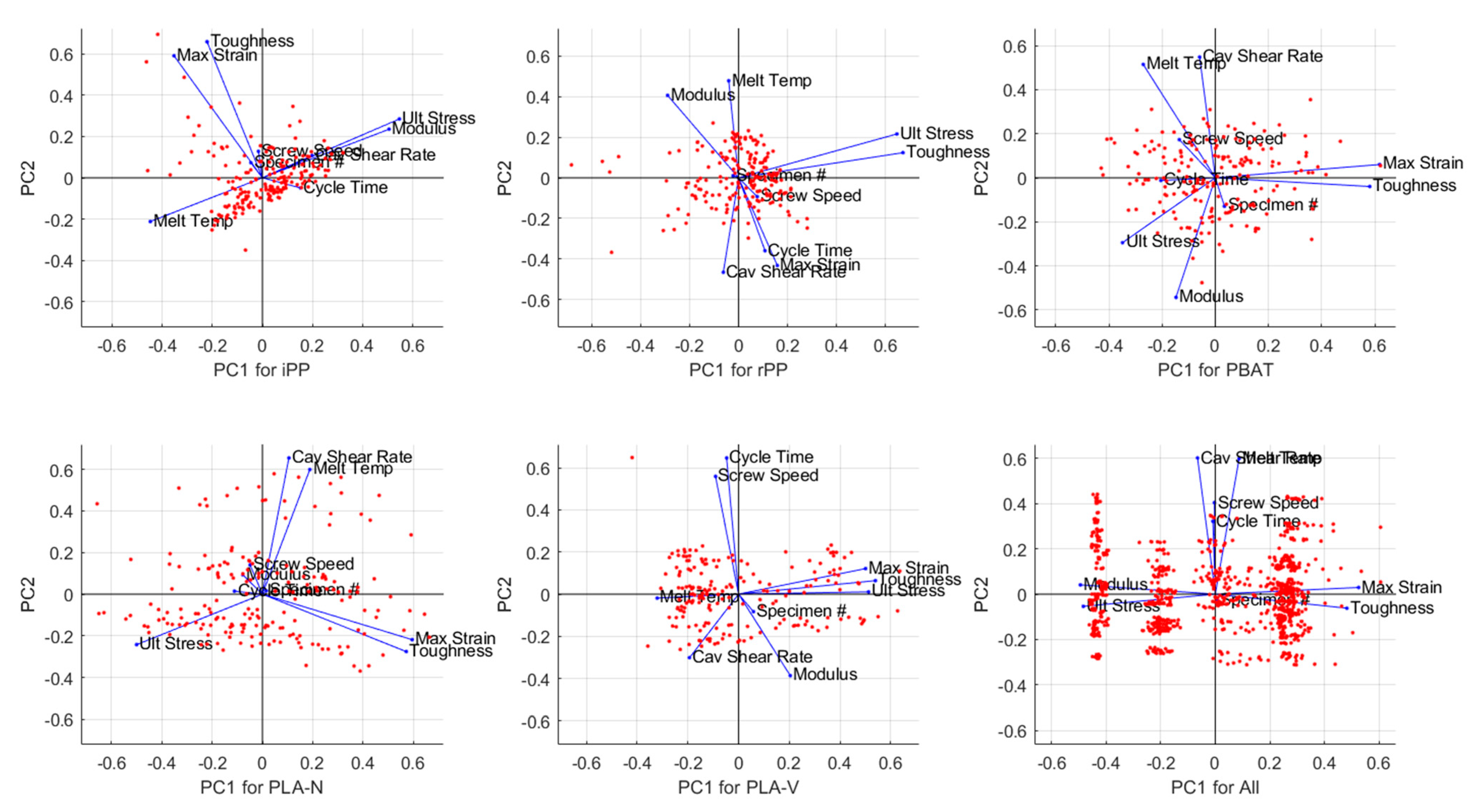
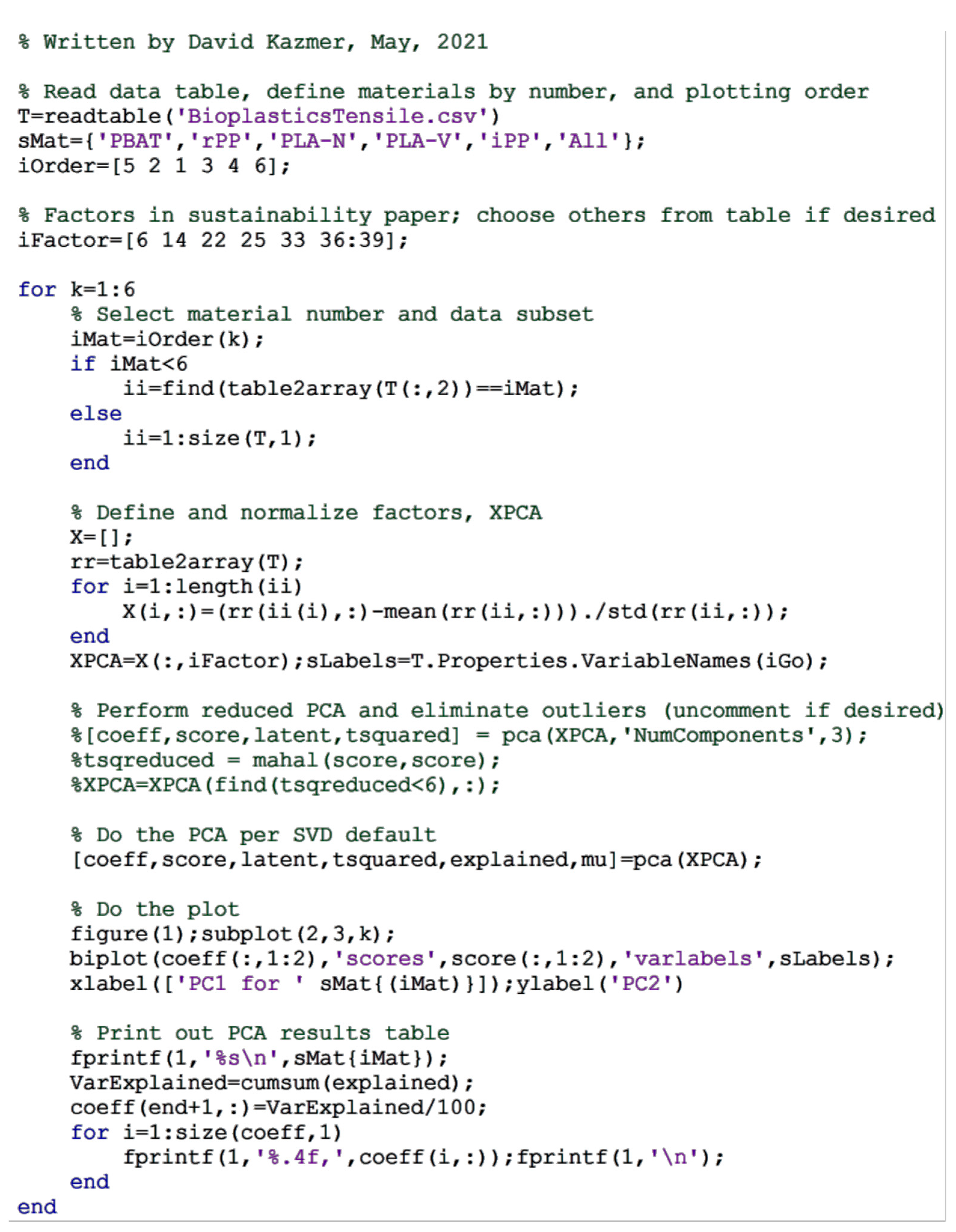
Appendix D. Principal Component Analysis Models

Table A22. Factors, principal component coefficients, and cumsum (R2, cumulative variation explained) for iPP.
FactorPC1PC2PC3PC4PC5PC6PC7PC8PC9
Cycle Time, s0.1527−0.04940.25710.68460.22430.6101−0.0584−0.1164−0.0021
Melt Temp, C−0.4473−0.21170.4644−0.03920.04580.06030.61370.39430.0058
Cav Shear Rate, s−10.19860.10780.6885−0.40160.23950.0144−0.48230.1530−0.0065
Screw Speed, %Max−0.01580.12800.36540.5290−0.4814−0.5631−0.14150.0352−0.0016
Specimen # (order)−0.04590.0724−0.07390.23800.8086−0.49910.0661−0.0361−0.0007
Max Strain, %−0.35280.59040.0168−0.0299−0.04010.1581−0.0214−0.10230.6987
Ult Stress, MPa0.54720.2845−0.18820.0938−0.00120.01400.16510.72900.1749
Modulus, MPa0.50580.23510.2615−0.1495−0.0351−0.07850.5781−0.50650.0034
Toughness, MJ/m3−0.22090.6581−0.0334−0.0073−0.04300.16280.03290.0804−0.6936
cumsum(R2)0.24810.46910.60130.71320.82320.92410.97160.99991.0000
Table A23. Factors, principal component coefficients, and cumsum (R2, cumulative variation explained) for rPP.
FactorPC1PC2PC3PC4PC5PC6PC7PC8PC9
Cycle Time, s0.1080−0.3599−0.0920−0.52730.21800.60160.28600.28470.0055
Melt Temp, C−0.04020.4787−0.4514−0.1471−0.19280.02880.6252−0.33910.0022
Cav Shear Rate, s−1−0.0622−0.46650.53010.0744−0.0027−0.14910.5128−0.4548−0.0030
Screw Speed, %Max0.0760−0.0928−0.20190.82500.18720.43200.19630.06310.0027
Specimen # (order)−0.02210.0105−0.2178−0.05290.8787−0.40920.0876−0.04260.0027
Max Strain, %0.1584−0.4332−0.37870.0800−0.3147−0.49680.25860.4516−0.1435
Ult Stress, MPa0.64630.21620.2118−0.00980.06820.01150.0375−0.0223−0.6956
Modulus, MPa−0.28970.40650.46000.06950.0659−0.06980.37770.61850.0021
Toughness, MJ/m30.67070.12380.13660.0083−0.0021−0.09530.08550.06510.7039
cumsum(R2)0.23150.39510.52710.63880.75020.85520.93890.99971.0000
Table A24. Factors, principal component coefficients, and cumsum (R2, cumulative variation explained) for PBAT.
FactorPC1PC2PC3PC4PC5PC6PC7PC8PC9
Cycle Time, s−0.2049−0.01250.6599−0.32060.4517−0.0630−0.2687−0.37330.0047
Melt Temp, C−0.27090.51490.24780.0069−0.0086−0.2040−0.18820.72310.0004
Cav Shear Rate, s−1−0.05890.54830.1828−0.0043−0.12280.69330.3633−0.1863−0.0030
Screw Speed, %Max−0.13490.1731−0.15720.66480.6548−0.11050.1838−0.1018−0.0004
Specimen # (order)0.0343−0.12950.50150.6605−0.4867−0.0490−0.1871−0.14130.0016
Max Strain, %0.61770.06030.1882−0.00030.1562−0.01440.07270.14030.7279
Ult Stress, MPa−0.3485−0.29460.2644−0.0816−0.0899−0.25640.77460.11750.1659
Modulus, MPa−0.1475−0.54350.09140.10920.23630.6251−0.13350.44370.0361
Toughness, MJ/m30.5806−0.03970.2826−0.01580.1638−0.04960.26170.2055−0.6643
cumsum(R2)0.26740.43580.55620.66870.77160.85760.93680.99991.0000
Table A25. Factors, principal component coefficients, and cumsum (R2, cumulative variation explained) for PLA-N.
FactorPC1PC2PC3PC4PC5PC6PC7PC8PC9
Cycle Time, s−0.11110.01420.5786−0.3447−0.3765−0.6036−0.01000.1661−0.0063
Melt Temp, C0.18870.5994−0.18540.0462−0.0916−0.0827−0.69440.2667−0.0040
Cav Shear Rate, s−10.10560.6552−0.00750.04230.00340.02390.69770.2650−0.0106
Screw Speed, %Max−0.04880.13990.2998−0.43670.82690.0406−0.10760.02060.0027
Specimen # (order)0.01580.01580.31130.80420.3262−0.3815−0.0304−0.0548−0.0030
Max Strain, %0.5957−0.21870.0762−0.02210.02850.01200.03540.24350.7277
Ult Stress, MPa−0.5000−0.2424−0.15190.10550.09910.0378−0.00870.79910.0840
Modulus, MPa−0.07770.09260.64080.1676−0.21640.6917−0.12780.07090.0090
Toughness, MJ/m30.5722−0.27590.0668−0.01140.04570.03420.02810.3531−0.6806
cumsum(R2)0.27910.46000.59310.70640.81240.90440.96040.99981.0000
Table A26. Factors, principal component coefficients, and cumsum (R2, cumulative variation explained) for PLA-V.
FactorPC1PC2PC3PC4PC5PC6PC7PC8PC9
Cycle Time, s−0.04710.64780.23890.2213−0.48830.47980.0470−0.0342−0.0025
Melt Temp, C−0.3209−0.01870.2612−0.0205−0.2186−0.42310.77480.02880.0101
Cav Shear Rate, s−1−0.1933−0.3018−0.15340.65050.31990.46330.32250.06140.0039
Screw Speed, %Max−0.09070.5599−0.0588−0.32940.70210.10990.24370.0424−0.0114
Specimen # (order)0.0589−0.08340.89470.18410.3204−0.0631−0.21920.01900.0081
Max Strain, %0.50050.1210−0.04770.1867−0.0153−0.15510.12060.7149−0.3845
Ult Stress, MPa0.51250.01080.00400.09610.0558−0.02840.2451−0.6763−0.4546
Modulus, MPa0.2038−0.38670.2102−0.5722−0.10840.57540.26740.1496−0.0262
Toughness, MJ/m30.53950.0640−0.02540.11640.0272−0.06480.1997−0.03610.8028
cumsum(R2)0.35800.48420.59760.70550.80870.89900.97450.99791.0000
Table A27. Factors, principal component coefficients, and cumsum (R2, cumulative variation explained) for all materials together.
FactorPC1PC2PC3PC4PC5PC6PC7PC8PC9
Cycle Time, s−0.00880.32220.5928−0.2100−0.6977−0.11710.0127−0.0008−0.0031
Melt Temp, C0.08730.5996−0.10350.09480.02900.77820.01120.0655−0.0484
Cav Shear Rate, s−1−0.06530.6028−0.51290.1912−0.1245−0.52830.0452−0.19000.0047
Screw Speed, %Max−0.00330.40430.4876−0.20210.7040−0.24820.0263−0.0008−0.0000
Specimen # (order)0.0064−0.02500.35750.93110.0190−0.0475−0.0454−0.0007−0.0016
Max Strain, %0.52570.0293−0.03640.0212−0.0174−0.07260.24410.32170.7432
Ult Stress, MPa−0.4840−0.05400.07050.01000.01940.16370.5514−0.51250.4048
Modulus, MPa−0.49460.0408−0.05240.0410−0.0142−0.06450.39000.7606−0.1195
Toughness, MJ/m30.4824−0.06220.01540.0200−0.0064−0.03810.6922−0.1225−0.5168
cumsum(R2)0.37620.50020.61320.72420.83150.93270.97810.99711.0000

References

  1. Alaerts, L.; Augustinus, M.; van Acker, K. Impact of bio-based plastics on current recycling of plastics. Sustainability 2018, 10, 1487. [Google Scholar] [CrossRef] [Green Version]
  2. Geissdoerfer, M.; Savaget, P.; Bocken, N.M.; Hultink, E.J. The Circular Economy—A new sustainability paradigm? J. Clean. Prod. 2017, 143, 757–768. [Google Scholar] [CrossRef] [Green Version]
  3. Sihvonen, S.; Partanen, J. Eco-design practices with a focus on quantitative environmental targets: An exploratory content analysis within ICT sector. J. Clean. Prod. 2017, 143, 769–783. [Google Scholar] [CrossRef]
  4. Morini, A.A.; Ribeiro, M.J.; Hotza, D. Early-stage materials selection based on embodied energy and carbon footprint. J. Mater. 2019, 178, 107861. [Google Scholar] [CrossRef]
  5. Ashby, M.F. Materials and the Environment: Eco-Informed Material Choice; Elsevier: Amsterdam, The Netherlands, 2012. [Google Scholar]
  6. Wu, X.; Hu, S.; Mo, S. Carbon footprint model for evaluating the global warming impact of food transport refrigeration systems. J. Clean. Prod. 2013, 54, 115–124. [Google Scholar] [CrossRef]
  7. Rydh, C.J.; Sun, M. Life cycle inventory data for materials grouped according to environmental and material properties. J. Clean. Prod. 2005, 13, 1258–1268. [Google Scholar] [CrossRef]
  8. Tucker, N.; Johnson, M. Low Environmental Impact Polymers; iSmithers Rapra Publishing: Shropshire, UK, 2004. [Google Scholar]
  9. Razza, F.; Briani, C.; Breton, T.; Marazza, D. Metrics for quantifying the circularity of bioplastics: The case of bio-based and biodegradable mulch films. Resour. Conserv. Recycl. 2020, 159, 104753. [Google Scholar] [CrossRef]
  10. Changwichan, K.; Silalertruksa, T.; Gheewala, S.H. Eco-Efficiency Assessment of Bioplastics Production Systems and End-of-Life Options. Sustainability 2018, 10, 952. [Google Scholar] [CrossRef] [Green Version]
  11. Blom, H.P.; Teh, J.W.; Rudin, A. PP/PE blends. IV. Characterization and compatibilization of blends of postconsumer resin with virgin PP and HDPE. J. Appl. Polym. Sci. 1998, 70, 2081–2095. [Google Scholar] [CrossRef]
  12. Tai, C.; Li, R.; Ng, C. Impact behaviour of polypropylene/polyethylene blends. Polym. Test. 2000, 19, 143–154. [Google Scholar] [CrossRef]
  13. Aumnate, C.; Rudolph, N.; Sarmadi, M. Recycling of Polypropylene/Polyethylene Blends: Effect of Chain Structure on the Crystallization Behaviors. Polymers 2019, 11, 1456. [Google Scholar] [CrossRef] [Green Version]
  14. Peelman, N.; Ragaert, P.; De Meulenaer, B.; Adons, D.; Peeters, R.; Cardon, L.; Van Impe, F.; Devlieghere, F. Application of bioplastics for food packaging. Trends Food Sci. Technol. 2013, 32, 128–141. [Google Scholar] [CrossRef] [Green Version]
  15. Ragaert, K.; Hubo, S.; Delva, L.; Veelaert, L.; Du Bois, E. Upcycling of contaminated post-industrial polypropylene waste: A design from recycling case study. Polym. Eng. Sci. 2017, 58, 528–534. [Google Scholar] [CrossRef]
  16. Kazmer, D. Injection Mold Design Engineering, 2nd ed.; Carl Hanser Verlag: Munich, Germany, 2016; p. 410. [Google Scholar]
  17. Jem, K.J.; Tan, B. The development and challenges of poly (lactic acid) and poly (glycolic acid). Adv. Ind. Eng. Polym. Res. 2020, 3, 60–70. [Google Scholar] [CrossRef]
  18. Wilkinson, R.W.; Dole, M. Specific heat of synthetic high polymers. X. Isotactic and atactic polypropylene. J. Polym. Sci. 1962, 58, 1089–1106. [Google Scholar] [CrossRef]
  19. Touati, N.; Kaci, M.; Bruzaud, S.; Grohens, Y. The effects of reprocessing cycles on the structure and properties of isotactic polypropylene/cloisite 15A nanocomposites. Polym. Degrad. Stab. 2011, 96, 1064–1073. [Google Scholar] [CrossRef]
  20. Schreiber, H.; Bagley, E.; West, D. Viscosity/Molecular weight relation in bulk polymers—I. Polymer 1963, 4, 355–364. [Google Scholar] [CrossRef]
  21. Jolliffe, I.T. Principal Component Analysis (Principal Component Analysis); Springer: New York, NY, USA, 2002; pp. 78–110. [Google Scholar]
  22. Wall, M.E.; Rechtsteiner, A.; Rocha, L.M. Singular value decomposition and principal component analysis. In A Practical Approach to Microarray Data Analysis; Springer: New York, NY, USA, 2003; pp. 91–109. [Google Scholar]
  23. Sokolnikoff, I.S.; Specht, R.D. Mathematical Theory of Elasticity; McGraw-Hill: New York, NY, USA, 1956. [Google Scholar]
  24. Peischl, G.C.; Bruker, I. Melt homogeneity in injection molding: Application of a ring-bar device. Polym. Eng. Sci. 1989, 29, 202–208. [Google Scholar] [CrossRef]
  25. Ge, T.; Robbins, M.O. Anisotropic plasticity and chain orientation in polymer glasses. J. Polym. Sci. Part B Polym. Phys. 2010, 48, 1473–1482. [Google Scholar] [CrossRef]
  26. Elduque, A.; Javierre, C.; Elduque, D.; Fernández, Á. LCI Databases Sensitivity Analysis of the Environmental Impact of the Injection Molding Process. Sustainability 2015, 7, 3792–3800. [Google Scholar] [CrossRef] [Green Version]
  27. Ayağ, Z.; özdem[idot]r, R.G. An analytic network process-based approach to concept evaluation in a new product development environment. J. Eng. Des. 2007, 18, 209–226. [Google Scholar] [CrossRef]
  28. Mulrennan, K.; Donovan, J.; Creedon, L.; Rogers, I.; Lyons, J.G.; McAfee, M. A soft sensor for prediction of mechanical properties of extruded PLA sheet using an instrumented slit die and machine learning algorithms. Polym. Test. 2018, 69, 462–469. [Google Scholar] [CrossRef]
Figure 1. Layout design of hot runner, two-cavity mold for producing ASTM tensile specimens.
Sustainability 13 08102 g001
Figure 2. Apparent viscosity of the five investigated materials indicated in Table 1 where the upward triangle, △, represents a material temperature of 180 °C and the downward triangle, ▽, represents 200 °C.
Sustainability 13 08102 g002
Figure 3. Thermal gravimetric analysis (TGA) results of the five investigated materials at temperatures ranging from 150 °C to 400 °C (heating ramp rate of 10 °C/min) in a nitrogen environment.
Sustainability 13 08102 g003
Figure 4. (top) Bounding stress–strain plots for iPP, rPP, PBAT, PLA-N, PLA-V as characterized by the (bottom) mean structural performance of specimens tested across the 32 DOE runs. Symbols represent DOE runs producing specimens with the (△) highest and (▽) lowest toughness.
Sustainability 13 08102 g004
Figure 5. Images of representative tested specimens for the (left) highest and (right) lowest specimens for each of the five investigated materials as indicated in the structural performance plot of Figure 4.
Sustainability 13 08102 g005
Figure 6. Summary of coefficient of variation (COV) and coefficient of determination (R2) for each of the five investigated materials. Multiple regression coefficients for the 20 models are provided in Appendix B.
Sustainability 13 08102 g006
Figure 7. Summary of the model coefficients (b) as normalized relative to the mean of each observed response of the five investigated materials. The model coefficients are provided in Appendix B.
Sustainability 13 08102 g007
Figure 8. Biplot of the first and second principal components (PC1 and PC2) for the five investigated materials and a sixth model of all material data together. PC weightings and statistics are provided in Appendix D.
Sustainability 13 08102 g008
Table 1. Overview of investigated materials including recommended melt temperature and mechanical properties.
ItemiPPrPPPBATPLA-NPLA-V
SupplierLyondellBasellKW PlasticsBio-FedNatureWorksVegeplast
GradePro-fax 702KWR621-20M-Vera GP1025W3052DFlex-AN 29
Recommended melt temperature, °C210200190205180
Melt for rate, g/10 min3520161450
Onset melt temperature, °C156153163163144
Peak degradation temperature, °C304350358350280
y 1 : Mean; SD tensile modulus, MPa997; 441130; 666274; 892703; 622298; 191
y 2 : Mean; SD ultimate stress, MPa16.04; 0.5715.66; 3.1563.17; 1.9354.69; 2.8612.97; 6.68
y 3 : Mean; SD elongation @failure, %56.44; 8.3652.72; 2.432.04; 0.145.95; 1.3934.3; 14.15
y 4 : Mean; SD toughness, MJ/m38.92; 1.318.14; 1.670.97; 0.082.67; 0.805.13; 4.50
Table 2. Factors and level settings implemented for the full factorial design of experiments.
Level
Setting
x 1 : Hot Runner and
Barrel Temperature
(°C)
x 2 : Cooling
Time
(s)
x 3 : Plastication
Speed
(% Maximum)
x 4 : Injection
Velocity
(mL/s)
118020259.25
2200 (or 220 for iPP)407518.5
3 39
4 78
Publisher’s Note: MDPI stays neutral with regard to jurisdictional claims in published maps and institutional affiliations.

