
Role of Model Predictive Control for Enhancing Eco-Driving of Electric Vehicles in Urban Transport System of Japan


Interdisciplinary Graduate School of Engineering Sciences, Kyushu University, Fukuoka 816-8580, Japan
*
Author to whom correspondence should be addressed.
Sustainability 2021, 13(16), 9173; https://0-doi-org.brum.beds.ac.uk/10.3390/su13169173
Submission received: 26 July 2021
/
Revised: 13 August 2021
/
Accepted: 13 August 2021
/
Published: 16 August 2021
(This article belongs to the Collection Electric Vehicles: New Challenges and Opportunities for Sustainability)
Abstract
:Electrification alters the energy demand and environmental impacts of vehicles, which brings about new challenges for sustainability in the transport sector. To further enhance the energy economy of electric vehicles (EVs) and offer an energy-efficient driving strategy for next-generation intelligent mobility in daily synthetic traffic situations with mixed driving scenarios, the model predictive control (MPC) algorithm is exploited to develop a predictive cruise control (PCC) system for eco-driving based on a detailed driving scenario switching logic (DSSL). The proposed PCC system is designed hierarchically into three typical driving scenarios, including car-following, signal anticipation, and free driving scenario, using one linear MPC and two nonlinear MPC controllers, respectively. The performances of the proposed tri-level MPC-based PCC system for EV eco-driving were investigated by a numerical simulation using the real road and traffic data of Japan under three typical driving scenarios and an integrated traffic situation. The results showed that the proposed PCC system can not only realize driving safety and comfortability, but also harvest considerable energy-saving rates during either car-following (16.70%), signal anticipation (12.50%), and free driving scenario (30.30%), or under the synthetic traffic situation (19.97%) in urban areas of Japan.
1. Introduction
1.1. Research Background and Significance
Following the Paris Agreement signed at COP21 in 2015 and to achieve the Sustainable Development Goals (SDGs), governments and industries around the world have been developing innovative solutions to intensify the development of a sustainable low-carbon society. The public road transport sector consumes about 20% of global energy and contributes nearly 25% of energy-related CO2 emissions [1]. Therefore, as one of the largest global emitters, improving the environmental performance of automobiles is the top priority. Vehicle electrification is one of the key technologies making revolutionary changes to the automotive industry. In Japan, the market share for electrified vehicles is approximately 30% [2], which brings about the highest level of contribution to realize a “Well-to-Wheel Emission”. However, the latest report issued by the Agency for Natural Resources and Energy in 2021 indicated that Japan generates the fifth-most CO2 emissions in the world, and 56% of CO2 emissions were from electricity production [3]. According to the Institute of Energy Economics Japan (IEEJ) [4], Japan’s electricity demand is expected to increase by around 132 TWh/year (15% growth) if all Japanese gasoline- and diesel-fueled vehicles shift to EVs. As a result, it is not advisable to rely solely on vehicle electrification targeting future electric mobility for sustainability.
Energy consumption during vehicle driving is not only pertinent to the status of the vehicle itself, but also subject to road conditions and the traffic situation. Moreover, it largely depends on the motion or driving behavior of the vehicle in a complex road traffic environment [5]. Eco-driving, as one of the conceptual control technologies, has been considerably noted due to its capability of reducing energy consumption in either the local microscopic or global macroscopic level [6,7]. The core concept of eco-driving is to improve vehicle energy economy on the premise of meeting the basic requirements of travel, such as time or speed limits. The main objective of eco-driving is to attain the best match between the host vehicle speed and the vehicle surroundings, including road environment and traffic flow, through the appropriate operation controlled by a driver or an autonomous driving system. Thus far, eco-driving has paved a new way for energy saving and emission reduction in road transport and has always been the focus of research in academia and industry.
Following the developing trend of connected and automated vehicles (CAVs) and intelligent transportation systems (ITSs), eco-driving assistance systems (EDAS), as the extension of advanced driver assistance systems (ADASs), present a transcendent energy economy improvement potential due to higher levels of engagement with the driving surroundings [8]. Involving autonomous driving features, the predictive cruise control (PCC) system is an ideal EDAS to take full advantage of the energy saving of eco-driving because of two reasons: (1) Equipped with an intelligent hardware system including controllers, sensors, and actuators, the cruise control system can partially or entirely replace the human driver to realize the energy saving objective automatically, which promotes the development of next-generation intelligent mobility; (2) Cruise control technology, as an embedded system into the EV, does not influence the energy-saving technologies of the EV itself, which means that the PCC system manipulates the EV to execute the eco-driving strategy that can be combined with the energy-saving technologies of the vehicle itself to maximize the energy-saving potential simultaneously [9].
1.2. Literature Review
The integration of eco-driving and intelligent driving originated from fuel-efficient cruise control, called predictive cruise control (PCC), in 2004 [10]. A representative research work done by E. Hellström et al. is the transportation task of a given route, in which the optimal control algorithm is applied to obtain the economic velocity [11]. Generally, eco-driving research combined with intelligent driving in urban transport systems can be categorized into three typical driving scenarios.
- Freeway-based eco-driving considering the road gradient to minimize fuel consumption
For freeway-based eco-driving, it mainly considers the influence of road terrain (road grade) on the vehicular fuel economy, planning the economic (or ecological) velocity of a single vehicle in a freeway driving situation without considering the influence from surrounding vehicles on the cruise vehicle.
Erik Hellström et al. [12,13,14,15] conducted a series of studies on the fuel economy problem of heavy trucks driving on a sloped road from 2005 to 2010 and developed a fuel-optimal look-ahead controller utilizing road topography information. This look-ahead controller took the weighted functions of fuel consumption, velocity variation, gear shifting, and braking times into the optimization objective function, transforming it into a dynamic programming (DP) problem. This research achieved higher fuel economy by generating smooth speed profiles with the result of fuel consumption reduction by 2.5%. However, this look-ahead controller needs to constantly search for the optimal control signal, which is computationally burdensome.
In 2011, Kamal et al. [16] utilized the model predictive control algorithm, combined with the information of road gradient, vehicle dynamics model, and fuel consumption model, to plan vehicular speed from passing up and down a hilly road. The results demonstrated that the fuel consumption could be effectively reduced by accelerating before climbing the uphill in a preplanned manner so as to avoid hard acceleration. In downslope, it takes advantage of the downhill gradient, and without any braking, the velocity is allowed to increase to some extent and finally settle at a specified speed.
In 2014, Yu [17] designed a hierarchical eco-driving system with two layers. The first layer applied the Dijkstra algorithm to optimize the average eco-speed at multiple signalized intersections considering traffic light information, traffic flow, and speed constraints at certain road sections. For the second layer, it considered the road slope information and calculated the real-time eco-speed.
The ACC InnoDrive system of Porsche adopted a similar method and achieved fuel consumption reduction of about 10% [18]. InnoDrive integrated an adaptive cruise control (ACC) system, GPS, and GIS to analyze driving intention based on real-time road traffic information. Then, the optimal velocity profile can be obtained based on the above information. Finally, it cooperatively controlled the engine, transmission, and braking system to follow the obtained optimal velocity profile to minimize fuel consumption.
- Urban roadway eco-driving considering traffic signal light information
In urban driving conditions, optimization of speed trajectory is performed to minimize fuel consumption by using upcoming traffic signal phase and timing (SPnT) information with the advancement of V2X technology, including Vehicle-to-Vehicle (V2V) communication and Vehicle-to-Infrastructure (V2I) interaction. Furthermore, the intelligent transport system (ITS) makes it possible to engage higher levels of real-time dynamic monitoring of the vehicle performance, enabling the eco-driving system to perform more efficiently.
In 2011, Asadi and Vahidi [19] proposed a vehicle-centered predictive cruise control system that controlled the vehicle based on traffic signal light information through the ITS to reduce the waiting time at the red interval of traffic signal lights and avoid unnecessarily frequent acceleration or deceleration. The simulation results showed that 47% fuel consumption and 56% CO2 emissions can be reduced by the predictive use of signal timing. In addition, this research offered the possibility of applying model predictive control (MPC) framework to formulate travel optimization considering the traffic signal light information.
In 2013, Kamal et al. [20] developed a comprehensive and innovative eco-driving model based on MPC, predicting the velocity of the preceding vehicle and taking into account the changing traffic signals at intersections to compute the optimal vehicle control input. The breakthrough of this research is that the MPC vehicle uses the upcoming signal status to choose its acceleration/deceleration behind a preceding vehicle to stop at a red signal by smooth deceleration instead of hard braking. The simulation results showed that up to 13.21% fuel savings could be achieved.
In 2015, De Nunzio et al. [21] further improved the energy efficiency for vehicles going through many successive signalized intersections. The presented pruning algorithm is capable of finding the energy-efficient path and returning the speed advisory to the drivers in a sub-optimal way. Although the simulated vehicles are independently equipped with the proposed algorithm and do not share information among vehicles, the noticeable traffic energy consumption reduction can be achieved without affecting travel time.
In 2019, an optimal parametric approach [22] was proposed to analytically solve an eco-driving problem for autonomous vehicles crossing multi-intersections without stopping. The traffic light information was described as spatial equality and temporal inequality constraints. The simulation results showed the advantages of considering multiple intersections jointly rather than dealing with them individually. An Ecological Adaptive Cruise Control (Eco-ACC) was proposed [23] to minimize energy consumption while avoiding collisions and complying with traffic signals, which was an extension of the conventional ACC system. In the higher-level controller, Eco-ACC computes the energy-optimal velocity reference incorporating red light duration. In the lower level, the ACC controller ensures safety against a collision with the preceding vehicle.
- Urban roadway eco-driving under car-following driving scenario
The development of optimal fuel economy under the circumstance of car-following requires considering the car-following safety. Due to the high unpredictability of driver behavior, the eco-driving cruise control under the mode of car-following is a more challenging task.
In 2006, Zhang and Ioannou [24] designed a PID controller for a truck-following system. This paper proposed that fuel consumption could be reduced by avoiding unnecessary acceleration and braking, and the goal of the controller was set to track the speed of the preceding vehicle while maintaining the specified inter-distance.
In 2008, Li et al. [25] took vehicle tracking and fuel efficiency into consideration in a study of adaptive cruise control. The research group used the inverse model to compensate for the nonlinearity of vehicle longitudinal dynamics. Given the tradeoff between fuel economy and vehicle tracking capability, the MPC framework was used to manage the optimization problem. The experimental results showed that the fuel-saving rate of the model is 8.8% and 2% on city roads and expressways, respectively.
In 2013, Kamal et al. [26] developed a new control system aimed at controlling the vehicle to improve its fuel economy in the changing urban transport system. By measuring the current road and traffic-related information, the system predicted the future traffic state of the preceding vehicle and calculated the optimal input signal into the vehicle. The experimental simulation results showed that the controller saved 13% fuel consumption in the urban traffic environment.
In 2019, Ma et al. [27] developed an ecological cooperative adaptive cruise control (eCACC) strategy to improve the fuel economy under V2V communication. The research work achieved better car-following performance results in significant energy savings in different driving cycles. In 2020, Nie and Farzaneh [28] proposed a multi-objective optimization ACC system for eco-driving based on the MPC algorithm, which dynamically computed an optimal acceleration command as the input to the host vehicle to realize driving safety, comfortability, and fuel consumption minimization. To reduce fuel consumption and emissions, considering the car-following scenario, Hu et al. [29] developed a model predictive multi-objective control framework and realized a 10.49% fuel consumption reduction. In 2021, Yang et al. [30] developed a car-following-oriented MPC controller with the purpose of maintaining a safe distance between the preceding vehicle while improving fuel economy.
Another approach for fuel efficiency is based on the utilization of new technologies. In 2007, Manzie et al. [31] proposed to remotely acquire the vehicle surrounding traffic information through an intelligent transportation system and thereby adjust driving strategy according to such required information. Experiments showed that the acquisition of remote traffic information enabled the vehicle with 7 s ahead preview capability, resulting in the improvement of fuel economy. In 2012, Li et al. [32] proposed a servo-loop control design of a Pulse-and-Gliding (PnG) strategy to minimize fuel consumption in the automated car-following scenario. Simulation experimental results showed that compared with the linear-quadratic (LQ)-based benchmark controller, the PnG controller improved the fuel economy by up to 20%.
1.3. What Will Be Elucidated in This Research
As reviewed so far, current existing research is mostly focused on eco-driving strategy development for specific driving scenarios, either car-following scenario, speed regulation based on traffic signal lights, or simply speed optimization considering road grade information. However, most of the time, a vehicle may experience an integrated traffic system with synthetic driving scenarios in an actual daily trip. For example, a common driving task may concern starting from an idling stop and accelerating to the maximum allowable speed in certain road section, during which the energy consumption is influenced by road gradient information. Moreover, when it is approaching a signalized intersection, the anticipation of an upcoming traffic signal phase and timing (SPnT) information directly affects the motion of the vehicle, during which the vehicle may follow a preceding vehicle to keep a safe driving distance. For such a common synthetic driving situation with various scenarios, a conventional eco-driving system solely designed for a specific driving scenario is far from meeting the requirements of handling and optimizing daily trips with the integrated traffic situation in urban transport systems. Hence, it is indispensable to develop a comprehensive eco-driving strategy that can automatically cope with multiple driving scenarios to minimize the energy consumption for the entire driving task.
Instead of taking various traffic constraints simultaneously and avoiding solving the complex global optimization problem once for all, a predictive cruise control system is designed hierarchically based on three MPC controllers: a linear MPC for the car-following scenario, a nonlinear MPC for the signal anticipation scenario, and another nonlinear MPC for the free driving scenario. A detailed driving scenario switching logic (DSSL) under the support of CAVs and ITS is formulated so that the proposed PCC system can automatically switch to the real-time driving scenario. Based on an artificial neural network (ANN) instantaneous EV energy consumption model (IECM), different optimization objectives can be defined for each driving scenario. For the car-following scenario, taking the driving velocity of the preceding vehicle into account, the control objectives of the linear model predictive controller (LMPC) include ensuring driving safety and comfortability of the host vehicle while minimizing the energy consumption. For the signal anticipation scenario, the control objective of the nonlinear model predictive controller (NLMPC) is to track an optimal reference velocity planned by a Reference Velocity Planning Algorithm based on upcoming SPnT information to pass the upcoming signalized intersection without any stop as well as reducing the energy consumption in approaching the intersection. For the free driving scenario, the control objective becomes integrating the gradient information of the road ahead to optimize the driving velocity of the host EV so that the energy economy can be enhanced.
Compared to the previous studies, the following originalities of this article can be highlighted:
- A comprehensive PCC system for EVs eco-driving was proposed based on a tri-level MPC algorithm and an ANN-ICEM.
- A detailed DSSL is designed so that the proposed tri-level MPC-based PCC system can automatically handle synthetic daily driving scenarios.
- The performance of the overall PCC system is investigated based on a customized simulation platform using real urban road and transport data in Japan.
- The role of MPC for enhancing the eco-driving of EV is explored and exploited.
The rest of this article is organized as follows. The problem formulation and overall proposed PCC system structure is demonstrated in Section 2. In Section 3, system modeling, tri-level MPC controller design and the corresponding optimization problem are explained. In Section 4, the establishment of the simulation platform and real urban road and transport data collection is introduced at first. Then, the simulation results are discussed in detail for each driving scenario and an integrated traffic situation with synthetic driving scenarios. Finally, the conclusion and future prospects are presented in Section 5.
2. Problem Formulation
To deal with the synthetic driving scenarios with multiple real driving constraints and realize the decoupled optimization for the different driving scenarios for the significance of practical implementation, the solution to design such a comprehensive eco-driving system for EV is to divide the mixed and coupled driving scenarios into three sub-scenarios, including free driving, car-following, and the signal anticipation scenario, instead of deriving the global optimal control for the overall driving task. The decoupling of each single driving scenario handled by the respective single MPC controller makes it possible to explore the internal mechanism and obtain the universal control strategy of MPC.
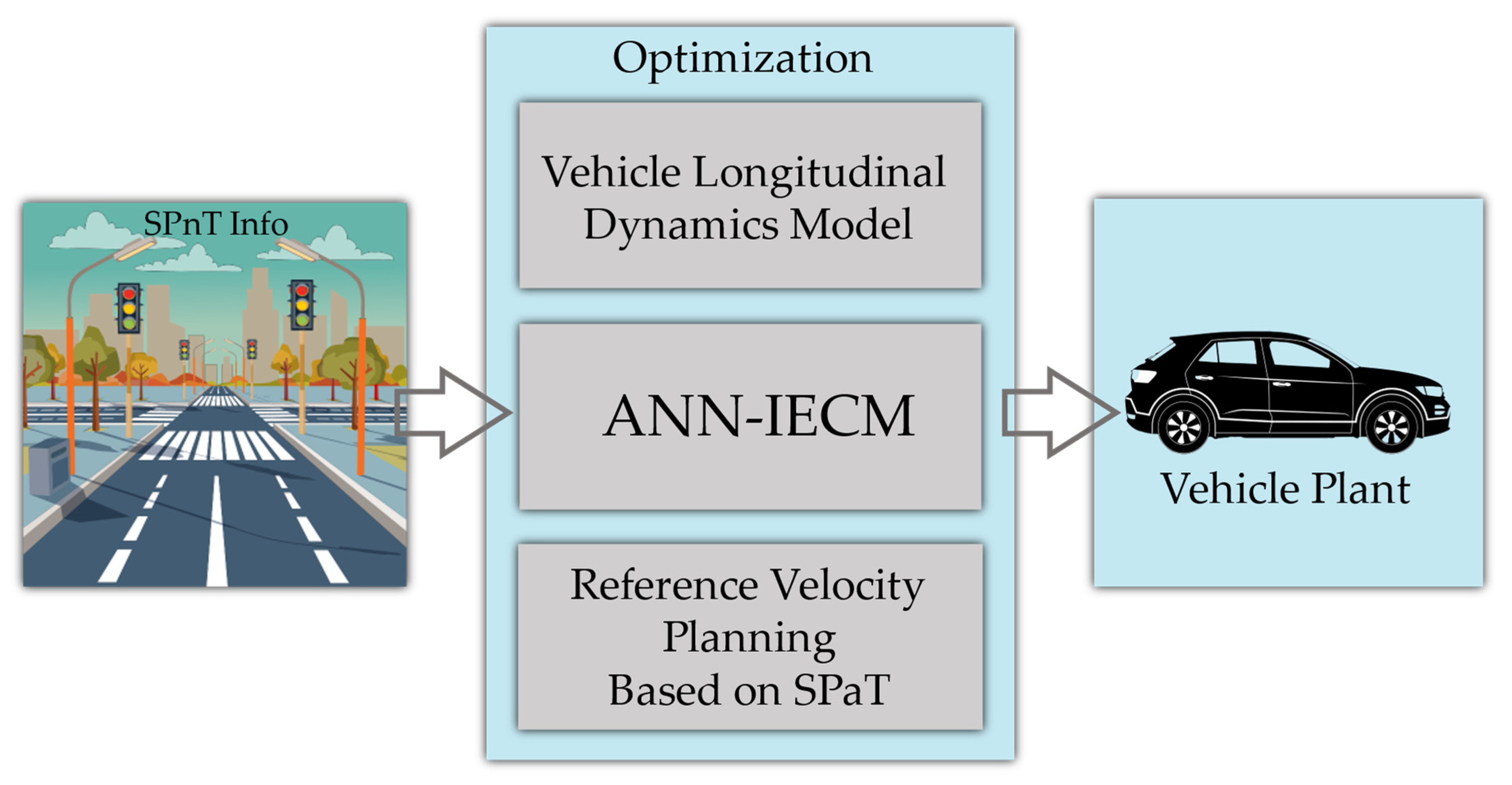
As illustrated in Figure 1, the schematic of the proposed tri-level MPC-based PCC system for eco-driving is designed based on the technical background of CAVs and ITS. The ITS enables Vehicle-to-Vehicle (V2V) and Vehicle-to-Infrastructure (V2I) communication for the host vehicle to access real-time road and traffic information in making optimal driving scenario switch decisions.
The V2V data interaction provides the real-time driving state information of the surrounding vehicles so that, e.g., in the car-following driving situation, the velocity of the preceding vehicle is crucial to the maintenance of safety distance. The data exchange used in this research includes real-time inter-vehicle distance or relative spacing between the host and preceding vehicle, , and the real-time velocity of the preceding vehicle . The real-time traffic and road conditions are important in working out an operative and eco-cruise strategy. The V2I communication realizes the real-time data transmission from the roadside to vehicle sides, such as driving speed limitation on certain road sections, the traffic signal phase and timing (SPnT) information, the distance to the upcoming signalized intersection, road altitude information according to the driving position, etc. In this research, the V2I interaction contains the dynamic distance to the upcoming signalized intersection , the speed limitation , the road altitude for certain driving position , the traffic signal lights state , and the remaining time for the current traffic signal light , as explained in Table 1.
As illustrated in Figure 1, the overall PCC system is distributed hierarchically. The perception of the driving environment for the host vehicle is supported by assumed ITS and CAVs, and these data streams are fed into the upper-level controller. The upper-level controller calculates the desired acceleration utilizing the optimization algorithm according to multiple control objectives based on the vehicle longitudinal dynamics model. The lower-level controller takes the desired acceleration obtained from the upper-level controller as input to adjust the throttle and brake pedal pressure and control the vehicle to track the desired acceleration. The main research content in this thesis is the upper-level controller design of the economic predictive cruise control system.
In actual daily trips, the proposed PCC system for eco-driving is required to automatically switch catering to different driving scenarios with different optimization objectives. Hence, a driving scenario switching logic (DSSL) is required to be designed precisely.
To formulate the DSSL of the host vehicle, a general vehicular braking distance model is firstly introduced [33] as follows:
where () refers to the braking distance, () denotes the minimum critical distance, () represents the host vehicle velocity at instant , () is the reaction time before braking, and () is the deceleration during braking.
The thresholds value for the distance to an upcoming signalized intersection and the relative distance between the host and preceding vehicles in the same lane are defined as and , respectively. They are numerically equal to the maximum braking distance based on Equation (2) using the parameters from [33], expressed as follows:
If the actual distance to the upcoming signalized intersection, , is greater than the threshold value, , as well as the actual relative distance between host and preceding vehicle, , greater than the threshold value, , the DSSL will switch into the free driving scenario, i.e., there is no need to consider the constraints from both the preceding vehicle and upcoming traffic signal light. However, once the becomes less than or equal to the , the motion of preceding vehicle has to be considered, i.e., the DSSL switching into car-following scenario. If the real-time is less than or equal to with greater than , either the signal anticipation scenario or free driving scenario will be selected by the DSSL. Otherwise, either the car-following scenario or free driving scenario will be selected. The critical factor is the upcoming traffic signal status and its remaining time to change from green light to red light. As long as the upcoming traffic signal is in the green interval and its remaining time is less than , the DSSL will select the signal anticipation scenario.
The real-time estimated time length to pass the upcoming signalized intersection is defined as follows:
where denotes the maximum physical allowable acceleration of the vehicle.
Thus, the detailed driving scenario switching logic (DSSL), shown in Figure 2, can be designed and used to switch into one of three studied typical driving scenarios.
The proposed predictive cruise control (PCC) system for eco-driving is based on the model predictive control algorithm. For each sampling time step, the MPC takes the state of the system at the current moment, solves a finite time-domain open-loop online optimization problem to obtain a sequence of desired acceleration within certain system constraints, and inputs the first element of the derived control sequence into the system to realize the closed-loop control, which inherently ensures the robustness of the control system. In the next time step, the rolling optimization problem is solved in real-time with the prediction horizon moving forward. Thus, repeatedly, the overall driving task with certain control and optimization objectives can be completed. The eco-driving system architecture based on the MPC algorithm for three typical driving scenarios is shown in Figure 3. The general vehicular longitudinal dynamics system includes an inter-vehicle longitudinal dynamics model and a vehicle dynamics model. The inter-vehicle longitudinal dynamics model describes the car-following behavior using a safety distance strategy and transfers the desired acceleration output by the MPC to the host vehicle.
To improve the system robustness for the designed MPC controller, a state observer is included to realize the feedback correction [34]. The error between the prediction value from the model and the actual measurement by state observer is taken to improve the prediction accuracy. In the above figure, the measured values of state and control of the controlled vehicle are and , respectively; the corresponding prediction values are and ; and the errors between them are defined as and .
3. Proposed MPC-Based Predictive Cruise Control System
According to the specific requirements for different driving scenarios proposed in Section 2, the corresponding system dynamics modeling is the prerequisite of developing the PCC system for eco-driving. For the free driving scenario and signal anticipation scenario, the electric vehicle longitudinal dynamics model is required to reflect the real-time vehicle driving condition. For the car-following driving scenario, the inter-vehicle longitudinal dynamics model is necessary to represent the coupling relationship between the host vehicle and the preceding vehicle. Once the DSSL switches into the signal anticipation scenario, the driving objective at this specific moment is to track the optimal reference velocity that is able to reduce the idling at red lights given the upcoming SPnT information. Therefore, a rule-based reference velocity planning algorithm that calculates an instantaneous optimal vehicle velocity trying to avoid stopping at the red light is proposed. Since the main target of the proposed PCC system is to evaluate energy consumption, an ANN-based instantaneous energy consumption estimation model (ANN-IECM) is applied.
3.1. System Modeling
The electric motor utilizes energy from the onboard battery to generate torque. Reversely, during vehicles’ braking, it works as a generator using regenerative braking power to recharge the battery. As the mapping of motor torque and rotation speed, electric motor efficiency can be expressed using the following formula [29]:
Then, the motor power can be calculated using defined motor efficiency as follows:
where .
The battery model can be simplified as an internal resistance model [35]. The is the internal resistance, is the equivalent current in the circuit, and is the open-circuit voltage. Thus, the battery power providing energy to electric motor can be obtained as follows [36]:
The variation rate of the state of charge (SOC), as an indicator of the remaining battery energy, is expressed as follows:
where denotes maximum battery capacity.
Substituting Equation (6) into Equation (7), the following equation can be obtained:
Consequently, the electric motor output torque can be calculated using power transition from the onboard battery and the electric motor as shown below:
When the motor output power is a positive value, the battery works in the discharging process. While is negative, the battery works in the charging procedure.
Therefore, the vehicle longitudinal dynamics is modeled based on the sum of all forces acting in the longitudinal direction, expressed as follows:
where denotes the equivalent vehicle mass, which is the sum of vehicle weight, driver, and rotational equivalent masses; is the traction force; is the rolling resistance coefficientis the air density; is the frontal area of the vehicle; and is the aerodynamic drag coefficient. is the electric motor output torque, is the single gear ratio of the gearbox, is the transmission efficiency, and is the radius of the vehicle wheel. is the road gradien and are the approximation coefficients of linearization. The related parameters used to model the electric vehicle are listed in Table 2.
For the car-following driving scenario, since the controlled plant is the inter-vehicle longitudinal dynamics, the prerequisite of developing the controller is to model the controlled plant. In this research, the inter-vehicle longitudinal dynamics model is designed, taking the inter-vehicle distance error, relative velocity, and acceleration of the host vehicle as state variables, desired acceleration of the host vehicle as a control input, and acceleration of the preceding vehicle as system disturbance. To calculate the desired acceleration, the state-space model between host and preceding vehicle is firstly established. The relative velocity between the host and preceding vehicle is defined as follows:
where and are the velocity of preceding and host vehicles, respectively.
The error of inter-vehicle distance, , is defined as:
where can be calculated using a customized variable time headway (VTH) as follows:
Then, we take the derivative of Equations (11) and (12):
where denotes the acceleration of the preceding vehicle and is the acceleration of the host vehicle. , , and are the constant coefficients and is the minimum inter-vehicle distance when the vehicles completely stop.
When applying the optimal desired acceleration obtained by the upper-level controller to the lower-level PI controller, there exists a time delay corresponding to the finite bandwidth of the vehicle’s dynamic response. To eliminate the time delay and process the obtained desired acceleration signal in time, the first-order lag model is used to model the inter-vehicle longitudinal dynamics.
where is the system gain, is the time constant, is the actual acceleration of the host vehicle, and is the optimal desired acceleration of the host vehicle.
Accordingly, the differential equation about desired and actual acceleration can be modeled as:
Taking the inter-vehicle distance error , relative velocity , and actual host vehicle acceleration as system state variables, we obtain:
Taking the calculated desired acceleration as the control input and acceleration of the preceding vehicle as system disturbance, the system state-space equation can be obtained as follows [28,37]:
where system matrices are derived as:
i.e.,
The discretized inter-vehicle longitudinal dynamics model can be expressed as follows [37]:
where refers to the th sampling time step, , , and are discretized system coefficient matrices, represents the system output, and is an identity matrix.
Assuming as the sampling period, , , and can be obtained as follows [37]:
When DSSL switches into the signal anticipation scenario, a reference velocity is required to be calculated based on the real-time driving state and upcoming traffic signal phase and timing information. The basic idea of calculating the is to accelerate when the time of green signal light is enough and decelerate until the start of the next green signal light so that the host vehicle can pass through the signalized intersection without any stop. According to research work [19], a non-empty intersection checking algorithm based on a set of logical rules is proposed.
Once entering the signal anticipation scenario, a vehicle plans to cross the first green interval of the upcoming traffic signal at the current time step with the velocity range:
where and denote the start time of the first red and green interval of the upcoming traffic signal light, respectively.
Then, the feasibility of crossing the signalized intersection using current velocity depends on if the above velocity range has the intersection with the allowable speed limits on a certain road section . If the set intersection is empty, the following green interval will be checked until a non-empty set intersection can be found. The mathematical expression of the “non-empty set intersection checking algorithm” is represented by [19]:
Finally, the reference velocity at each time step can be obtained by the following rule:
An instantaneous energy consumption estimation model (IECM) based on machine learning data mining is proposed catering to the driving characteristics of the electric vehicle. After smoothing the real chassis dynamometer experimental Drive Cycle data and determining the network structure, the Levenberg−Marquardt training algorithm [38] is applied to train the neural network and encapsulate it as a callable function.
Datasets used to develop the ANN-based IECM were derived from the Downloadable Dynamometer Database and were generated at the Advanced Mobility Technology Laboratory (AMTL) at Argonne National Laboratory for funding and guidance from the U.S.
As shown in Figure 4, using the artificial neural network as the fitting tool, the IECM takes motor torque , motor speed , transient vehicle velocity , and transient vehicle acceleration as input features to calculate the mapping output instantaneous energy consumption .
Note that the IECM is proposed mainly to develop the predictive cruise control system for eco-driving to evaluate the instantaneous energy economy for specific driving conditions. Therefore, to ensure the interactivity between each part of the PCC system, the well-trained ANN-based IECM is deployed in the MATLAB environment as a callable function as below:
Details of the validation of the IECM are described in Appendix A.
3.2. Tri-Level Model Predictive Controller
3.2.1. LMPC for Car-Following Scenario
As the key component of the entire predictive cruise control system, the car-following driving scenario is the most frequent and typical driving condition. In following the preceding vehicle, driving comfortability and energy economy are also required to be considered. Hence, in this section, the predictive cruise control system for EV eco-driving is designed based on MPC, taking the inter-vehicle longitudinal dynamics model as the control plant. By integrating the driving state of the preceding vehicle and the safety distance model, the motion of the host and preceding vehicle can be predicted within the prediction horizon. Based on ensuring the car-following safety, the energy economy is maximized. The cost function is established considering both driving safety and comfortability. By means of using the rolling horizon optimization algorithm, the optimal control value, i.e., the desired longitudinal acceleration, can be obtained, which is further fed into the vehicle longitudinal dynamics model. The controller structure of the car-following scenario is shown in Figure 5.
During the car-following process, energy consumption is closely related to the longitudinal acceleration. Hence, by smoothing the acceleration and jerk to reduce hard acceleration and deceleration, the energy economy can be efficiently improved. The derivative of vehicle acceleration can be defined as jerk:
The control objective can be mathematically expressed as:
where is the transient acceleration of the host vehicle and is the transient jerk of the host vehicle.
According to the analysis by Li [33], an approximate linear relation between energy consumption and vehicle acceleration can be found. Thus, here the energy economy can be quantified using the Euclidean norm for desired acceleration and desired jerk of the host vehicle:
where is the performance index of the energy economy, is the weight coefficient of desired acceleration, and is the weight coefficient of the desired jerk. For the former term, by minimizing , the acceleration amplitude can be lowered so that the energy economy can be improved. For the latter term, it limits the frequent acceleration or deceleration of the electric motor so as to further improve the energy economy. Besides, lowering the jerk can efficiently reduce the longitudinal driving impact so that driving comfortability can be improved.
Driving safety is always the top priority. In the previous section, the desired car-following model has been proposed based on a customized safety distance model. The control system regulates the vehicle to reach the desired car-following distance by manipulating its acceleration based on the V2V state information. Apart from the desired car-following distance calculated by the safety distance model as the ultimate control objective, another real-time safe distance, , before reaching the final desired value is required to constrain the actual inter-vehicle distance. To ensure driving safety and keep the host vehicle from a collision with the preceding vehicle, the actual car-following distance should always be greater than the safety distance . This real-time safe distance can be defined by a Time-to-Collision (TTC) strategy, which is used to describe the car-following safety during braking; e.g., when the host vehicle velocity is much greater than the preceding vehicle, it is still risky to collide with the preceding vehicle even if there is a long inter-vehicle distance. Therefore, the safety constraints can be defined as follows:
where is the actual real-time inter-vehicle distance and is the time to collision.
When the preceding vehicle is running at a steady state, the control objective is forcing the actual inter-vehicle distance to approach the desired safety distance calculated by the safety distance model, i.e., the error between and approaching zero. Simultaneously, to keep the traffic flow as stable as possible, another control objective is to let the host vehicle’s velocity approach the preceding vehicle’s velocity by adjusting the acceleration of the host vehicle, i.e., approaching zero.
To quantitatively describe the car-following capability, the Euclidean norm of and is used to define the cost function of driving safety:
where is the performance index of driving safety, is the weight coefficient of the tracking distance error, and is the weight coefficient of the relative velocity.
However, corresponding to the unstable driving condition of the preceding vehicle, the host vehicle tends to reflect this as hard acceleration or deceleration, which is against energy economy. If the weight of fuel economy is greater than driving safety in the final cost function, it is possible to compromise the vehicle dynamics in pursuing the energy economy. Therefore, the variables and are constrained by the following boundary conditions:
where and are the lower and upper boundary of inter-distance error, and are the extreme value of relative velocity, and and are the driver’s sensitivity to the and , which can be calculated by [38]:
where and are the coefficients of first-order terms and and are the constant terms.
Driving comfortability is presented in two aspects: (1) desired acceleration calculated by the upper-level controller should be aligned with the driver’s expectation; (2) the vehicle should maintain a constant speed whenever possible and avoid frequent acceleration or deceleration. Therefore, the following control objective can be defined:
where and are the desired acceleration boundary condition and and are the desired jerk boundary condition, respectively.
Moreover, considering the physical limitation of vehicle velocity and acceleration, the control inputs into the host vehicle should be constrained by:
where , , , and are all decided by the braking and acceleration capability of the vehicle itself.
Consequently, in this research, driving comfortability is realized by constraining the host vehicle acceleration as follows:
where is the performance index of driving comfortability and is the weight coefficient of the host vehicle longitudinal acceleration.
In the car-following scenario, the energy economy, driving safety, and comfortability are mutually restricted and affected. To obtain the optimal control value, each performance index is required to be considered cooperatively. Therefore, under the car-following scenario, the optimization problem of LMPC in each sampling period can be integrated as:
where is the system cost function under car-following scenario.
Replacing the and with and , respectively, the following equation can be obtained:
where is the weight matrix of the output vector:
As the input to the inter-vehicle longitudinal dynamics model, the comfortability constraints can be directly transformed into constraints of system inputs, as follows:
Then, can be substituted, and the driving safety constraints can be transformed into system output constraints:
For boundary condition 32, it can be transformed into system output constraints:
Until this point, the multi-objective optimization for the car-following scenario is well-designed. For each sampling time, such an overall optimization problem, including cost function and various constraints, can be transformed into a predictive form and quadratic programming problem and solved using the encapsulated function “quadprog” within MATLAB to realize the closed-loop control.
3.2.2. NLMPC for Signal Anticipation Scenario
When the host vehicle is driving in the signal anticipation scenario based on the DSSL, the predictive cruise control system enters the optimization problem defined in Equation (44), within the nonlinear equality constraints (45)~(46), and linear inequality constraints (47)~(51). At each sampling time , a reference velocity is obtained based on the reference velocity planning algorithm using real-time SPnT information, which is a velocity that can pass the upcoming signalized intersection without any stop, i.e., it always captures the green timing of traffic lights crossing the intersection. The cost function in Equation (44) takes the obtained reference velocity to execute the optimization. The first term of Equation (43) is to minimize the energy consumption of the vehicle during the signal anticipation. If only the first term exists, the vehicle would have no moving motivation because the first term forces the vehicle to consume as little energy as possible. Therefore, the second term is required to penalize the error between actual driving velocity and reference velocity so that the host vehicle can track the reference velocity at each moment in the signal anticipation scenario to realize the passing of the signalized intersection without any stop and further minimize the energy consumption. The third term is introduced with the slack factor to minimize the variation rate of acceleration/jerk, so that the driving comfortability during signal anticipation scenario is guaranteed. The velocity is bounded with the road section speed limitation in Equation (47). The vehicle acceleration, motor torque, and motor speed are all limited by the technical characteristics of the vehicle itself in Equations (48), (50) and (51), respectively. After solving the nonlinear optimization problem with nonlinear constraints in each time step, an optimal control sequence can be obtained, using the first control in the sequence as the vehicle’s input. Such a nonlinear online optimization is rolling forward with the moving of the prediction horizon to achieve real-time reference velocity tracking to minimize energy consumption. The controller structure of the signal anticipation scenario is shown in Figure 6.
Rewriting the electric vehicle longitudinal dynamics model into a state equation results in the following:
The cost function is defined as:
Therefore, the performance index can be expressed as:
s.t.
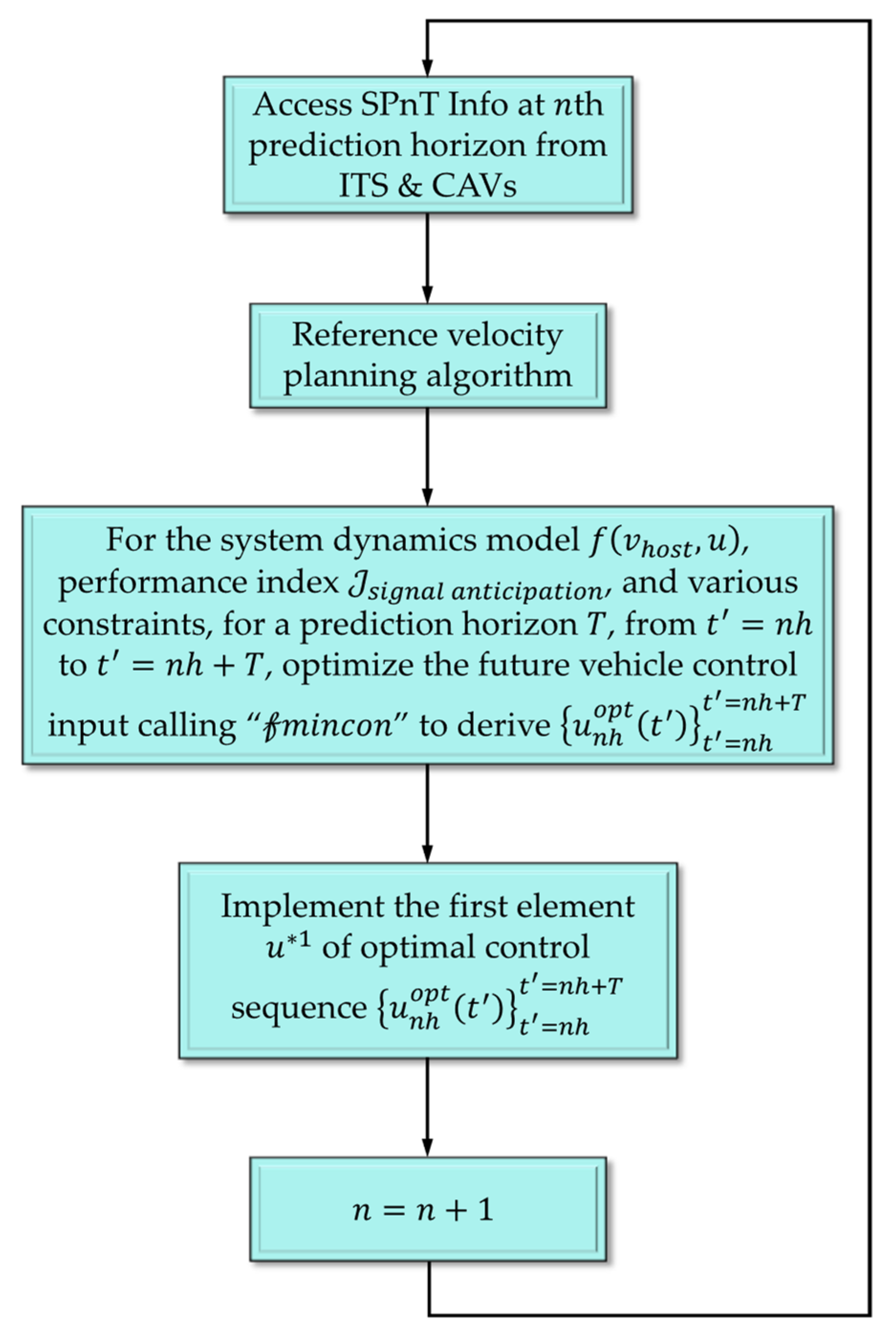
During the prediction horizon , the weights here , , and are chosen with the criterion that optimal magnitudes of cost terms are balanced. Finally, the weights can be tuned through the observation of simulation results to maximize the energy economy. To solve the above nonlinear optimization problem and derive the optimal control sequence, the encapsulated function “” with sequential quadratic programming (SQP) algorithm from MATLAB is called. The workflow of the MPC problem for the signal anticipation scenario is shown in Figure 7.
3.2.3. NLMPC for Free Driving Scenario
When the driving scenario switching logic (DSSL) selects the free driving mode, the vehicle starts eco-driving in the scenario, accessing the upcoming road gradient information. The basic concept is that a predictive cruise control system utilizes the vehicle longitudinal dynamics model combined with ANN-IECM to calculate the optimal control input based on the information of specific road altitude of the driving position to improve the energy economy over a free-travel distance. In the real implementation, the information of real-time road altitude is provided by ITS. The basic concept of the free driving scenario is demonstrated in Figure 8.
Based on the electric vehicle longitudinal dynamics model, the state-space equation of the electric vehicle in the free driving scenario can be expressed as:
The road gradient can be calculated using the real-time road altitude information as [20]:
The cost function in the free driving scenario is defined as:
The performance index thereby can be written as:
s.t.
where the most important parameter is the . Basically, the efficiency of the electric motor is relatively stable, which features a broad high-efficiency range and energy conversion efficiency. However, the power in the high rotation speed will decline, and the aerodynamics resistance will be the main source of energy consumption when the vehicle velocity is faster than . Therefore, the most energy-efficient driving velocity for an electric vehicle will be . Hence, the for the free driving scenario is set by ().
is the prediction horizon of the MPC algorithm during which the optimal control inputs are calculated, and is the optimal acceleration command. Given the performance index in Equation (55), is discretized into steps with size . For each prediction horizon, the future vehicle control sequence is obtained. Then, the first element of the sequence is input into the vehicle plant. The first term in the cost function is to minimize the overall energy consumption during the prediction horizon . The second term is to penalize the deviation of the actual vehicle velocity from the desired energy-efficient velocity . The third term is the cost for acceleration command to avoid hard input because of tracking the desired velocity. , , and are the weight factors for each term, respectively.
Similarly, the encapsulated function “𝓯mincon” with sequential quadratic programming (SQP) algorithm from MATLAB is called to solve this nonlinear optimization problem. The workflow of the MPC problem for the free driving scenario is demonstrated in Figure 9.
4. Results and Discussion of Case Studies
4.1. Establishment of Simulation Platform Based on CarSim and MATLAB/Simulink
CarSim is a software that precisely predicts the performance of the vehicle in response to driver controls in a user-defined environment. It provides integrated vehicle dynamics simulation for EVs. MATLAB/Simulink is more focused on the development of the control system. The connection port provided within CarSim makes it possible to link with MATLAB/Simulink. Therefore, the co-simulation based on these two platforms enables the accurate and flexible development of the PCC system for EVs eco-driving.
To begin with, the simulation platforms for three representative driving scenarios (car-following scenario, signal anticipation scenario, free driving scenario) are established, respectively. The first step is conducting parametric modeling within CarSim according to the configuration Table 2 and Table 3, and then setting the inputs and outputs of the vehicle dynamics model, shown in Figure 10.
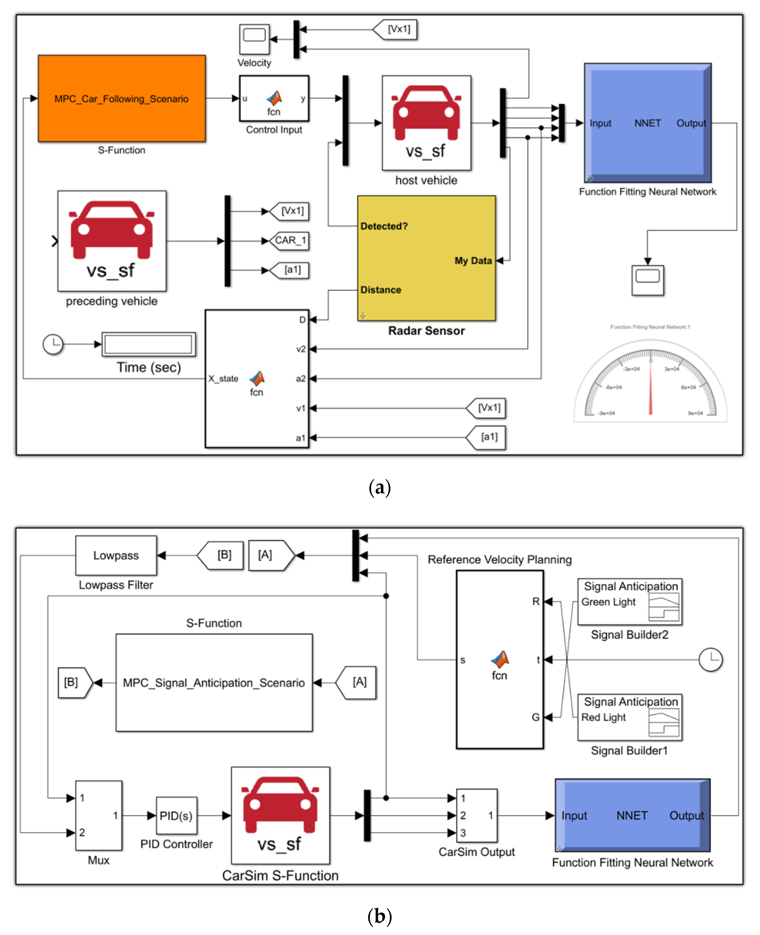
Once completing the settings within CarSim, the “Send to Simulink” button can connect CarSim with the MATLAB/Simulink. Then, the detailed predictive cruise control system can be developed within the Simulink environment. The visualization of three typical driving scenarios is intuitive to check the performance of the overall system, shown in Figure 11. The respective simulation environments are shown in Figure 12a–c.
The core MPC algorithms were written as S-Function, so that the required optimization problem solver “quadprog” and “fmincon” could be successfully called. The lower-level controllers which accept the optimal acceleration command are designed using a PID controller. The ANN-IECM is embedded in the MPC algorithm as a callable function and deployed as a portable Simulink block to explicitly show instantaneous energy consumption. The external data, such as the SPnT information and the road altitude information, can be imported using Signal Builder Block.
4.2. Real Road and Transport Data Collection in Urban Area of Japan
For the signal anticipation scenario, the simulative parameters of the traffic signal lights were configurated based on real data. The SPnT information was collected at Takeshita road, located near Hakata station in Fukuoka, Japan. There were seven traffic lights. The signal phase and timing information were collected through analyzing the videos which were recorded by cameras. The position of the traffic lights can be obtained using the Google Maps distance measurement tool.
For the car-following scenario and free driving scenario, the required real-world data includes the speed profile of the preceding vehicle and road elevation information. The required data, such as road elevation, driving position, driving velocity and acceleration, can be acquired from built-in sensors on a smartphone using MATLAB Mobile Version. Then, the collected data can be streamed directly to the Cloud being used by MPC online optimization of the proposed PCC system. The flow chart of data acquisition and transmission is shown in Figure 13.
4.3. Real Case Study for Car-Following Driving Scenario
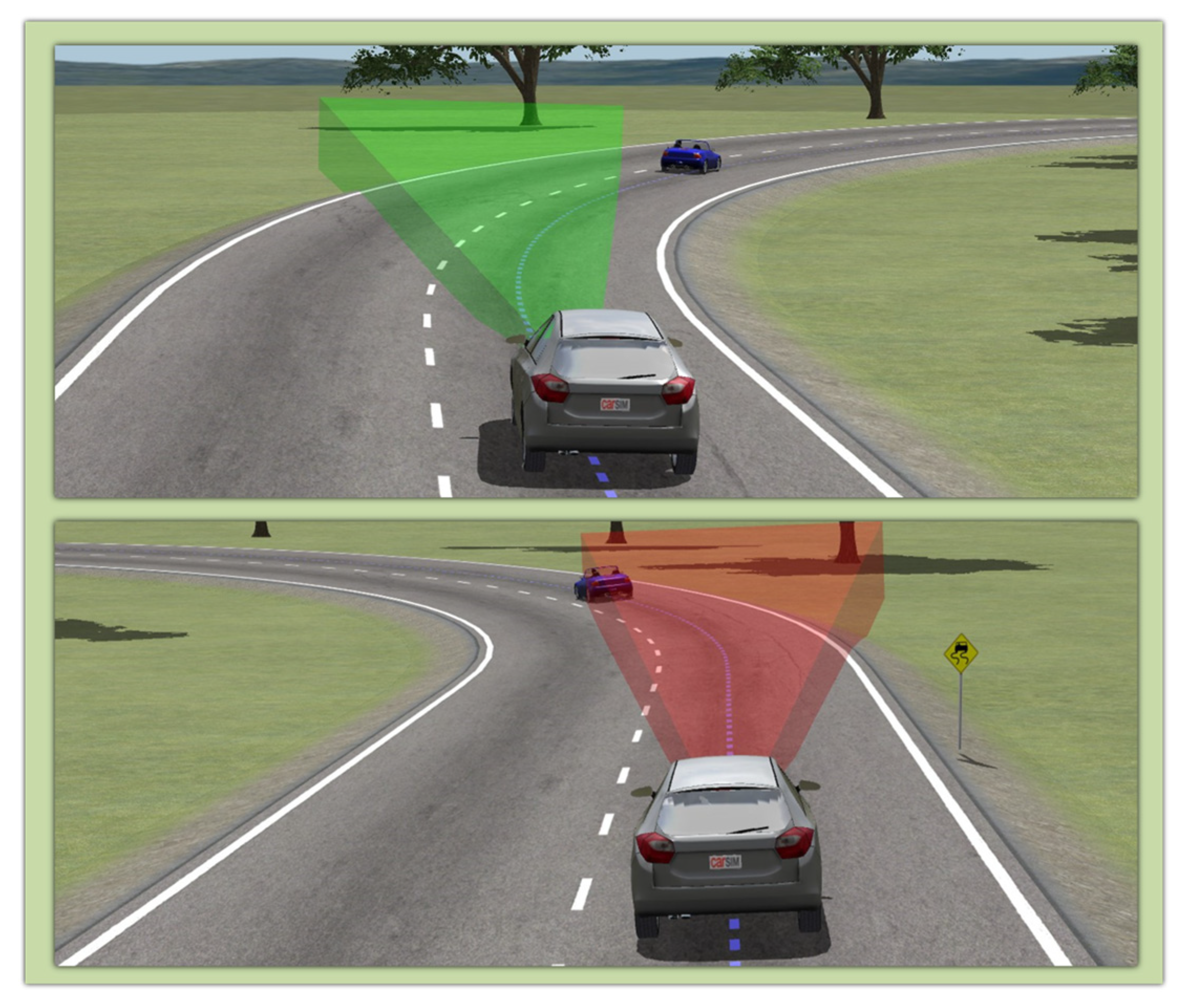
To test the stability of the car-following performance of the proposed PCC system, a velocity profile that fluctuated from 19.5 to 29.5 and finally decelerated to a complete stop within 50 s was recorded and taken as the velocity of the preceding vehicle. During the driving of the host vehicle, if the preceding vehicle is within the radar detection range, then the PCC system will automatically control the velocity of the host vehicle to follow the preceding vehicle. The real-time driving scenario is visualized in Figure 14. The initial velocity of preceding and host vehicles is and , respectively. The initial inter-vehicle distance is , which is larger than the desired inter-vehicle distance. The corresponding velocity comparison, relative position, battery state-of-charge (SOC), instantaneous energy consumption, and preceding vehicle detection state are shown in Figure 15.
From the first plot of Figure 15, with the velocity decrease of the preceding vehicle from 2 s to 7 s, the host vehicle reacted by slowing down the velocity as well, which demonstrated effective following performance of the PCC-controlled host vehicle. As shown in the fifth plot, from 11 s to 39 s, the preceding vehicle was not detected by the host vehicle PCC system. Therefore, the host vehicle cruised with the driver at a set velocity of 25.8 . Starting from 39 s, with the braking of the preceding vehicle, the preceding vehicle was again detected by the host vehicle, which triggered the car-following function of the PCC system. Therefore, the host vehicle also decreased its velocity. From the third plot, the battery state of the preceding vehicle finally settled at 78.4%, while the SOC of the host vehicle finalized at 78.8%. Therefore, it can be concluded that during this specific driving scenario, the energy consumption reduction was realized by 16.7% from the cumulative energy consumption. From the second plot, the acceleration of the host vehicle with the PCC system is limited within a certain range to guarantee driving comfortability. By contrast, the acceleration of the preceding vehicle without the PCC system features aggressive variation, which will make the driver feel uncomfortable. As a result, in the car-following scenario, an MPC-based PCC system can ensure the reduction of energy consumption as well as driving safety and comfortability due to the explicit consideration of input and output constraints and optimization-based control law design.
4.4. Real Case Study for Signal Anticipation Scenario
The case study for the signal anticipation scenario was conducted for the real road sections in the area located in the core commercial district, which is shown in Figure 16. The selected location is characterized by an average traffic flow movement of 8.3 to 13.8 during low traffic flow situations and 9.7during high traffic flow. The situation of different times directly influences the running condition of the preceding vehicle. Seven traffic signal lights were considered in the SPnT data collection process. Assuming that only the host and preceding vehicles were operating during simulation, without considering the constraints of other vehicles, the host vehicle maintained a safe distance from the preceding vehicle using the function of car-following of the PCC system.
During the low traffic flow situation, the host vehicle reacted to the acceleration of the preceding vehicle from 60 s. It follows that the PCC system switched to the signal anticipation scenario to track the reference velocity optimized by upcoming traffic SPnT information to avoid coming to a red interval. After 320 s, the preceding vehicle implemented a sharp deceleration. However, by managing the velocity of by PCC system, the host vehicle avoided the arrival at the signalized intersection during the red interval. After 580 s, the traffic flow became heavier. It is clear to see that after a stop in front of the red interval from 720 s to 735 s, the preceding vehicle started to accelerate. However, the host vehicle deployed by the proposed PCC system crossed the signalized intersection without any stop through managing the driving velocity in advance. A sharp deceleration was implemented by the preceding vehicle because of the upcoming red interval from 870 s to 890 s, during which the host vehicle was controlled by the PCC system to avoid encountering the red-light interval. Starting from 1000 s, the signal anticipation scenario began again to track the reference speed and successfully passed the signalized intersection without any stop. However, the preceding vehicle without velocity optimization had to experience a stop at around 1010 s. Figure 17 shows the space−time diagram, which visualizes the behavior of both the host and preceding vehicles during the overall driving task. It can be intuitively seen that the preceding vehicle without PCC system executed five times of stopping in front of the red-light interval. Comparatively, the host vehicle equipped with the proposed PCC system can always pass the signalized intersection during green-light interval by optimizing the driving velocity. According to instantaneous energy consumption, 12.5% cumulative energy savings were realized by the proposed PCC system.
4.5. Real Case Study for Free Driving Scenario
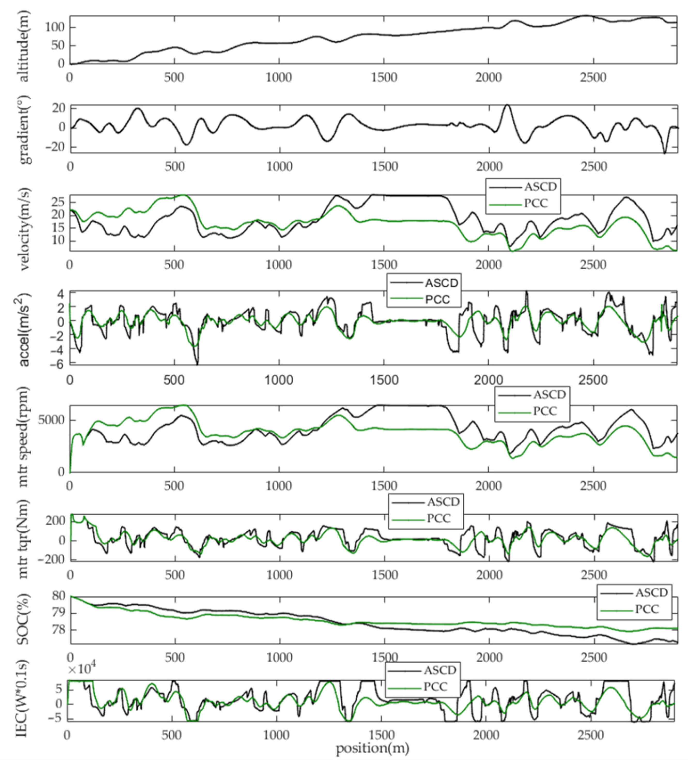
The test for the free driving scenario is conducted on a hilly road section covering 2.9 in total. The simulated scenario is visualized in Figure 18. The global coordinate of this hilly road section is shown in Figure 19. The comparative analysis was conducted between the driving pattern controlled by the proposed PCC system and the automatic speed control drive (ASCD). The initial velocity was the same for both driving patterns, set as 22.1. The altitude, gradient of the road section, velocity comparison of both driving patterns, acceleration comparison, instantaneous motor speed and motor torque comparison, battery SOC, and instantaneous energy consumption are shown in Figure 20.
From the first plot, it is known that the overall elevation exhibited an upward trend. The corresponding road gradient information can be obtained from the second plot, with the gradient range of −26~23°. Because of the PCC system, the velocity of the PCC-vehicle varied around the desired velocity 15. The optimized acceleration of the PCC-vehicle presented a smoother variation trend. Based on the gradient plot and acceleration plot, the basic rules can be concluded that the PCC-vehicle always accelerated just before the upslope, instead of accelerating while climbing the slope. When driving on the downslope section, the PCC-vehicle tends to rely on the inertia of the vehicle to drive, which was in line with the principle of eco-driving behavior. From the results of battery state-of-charge, it can be calculated that the baseline ASCD vehicle finalized at 77.2%, while the PCC-vehicle settled at 78.3%. The cumulative energy consumption for the baseline ASCD vehicle can be obtained as 2.63 , while the PCC-vehicle consumed 1.83 in total. The energy-saving was estimated as 30.3%. Here, in this case study, both the baseline ASCD vehicle and PCC-vehicle are electric vehicles with a regenerative braking system, which means that during the braking process, the vehicles can be charged instantaneously. The instantaneous energy consumption (IEC) also shows negative values. Therefore, the 30.3% energy savings rate was already considered in the charging process.
4.6. A Comprehensive Case Study in Synthetic Driving Scenario
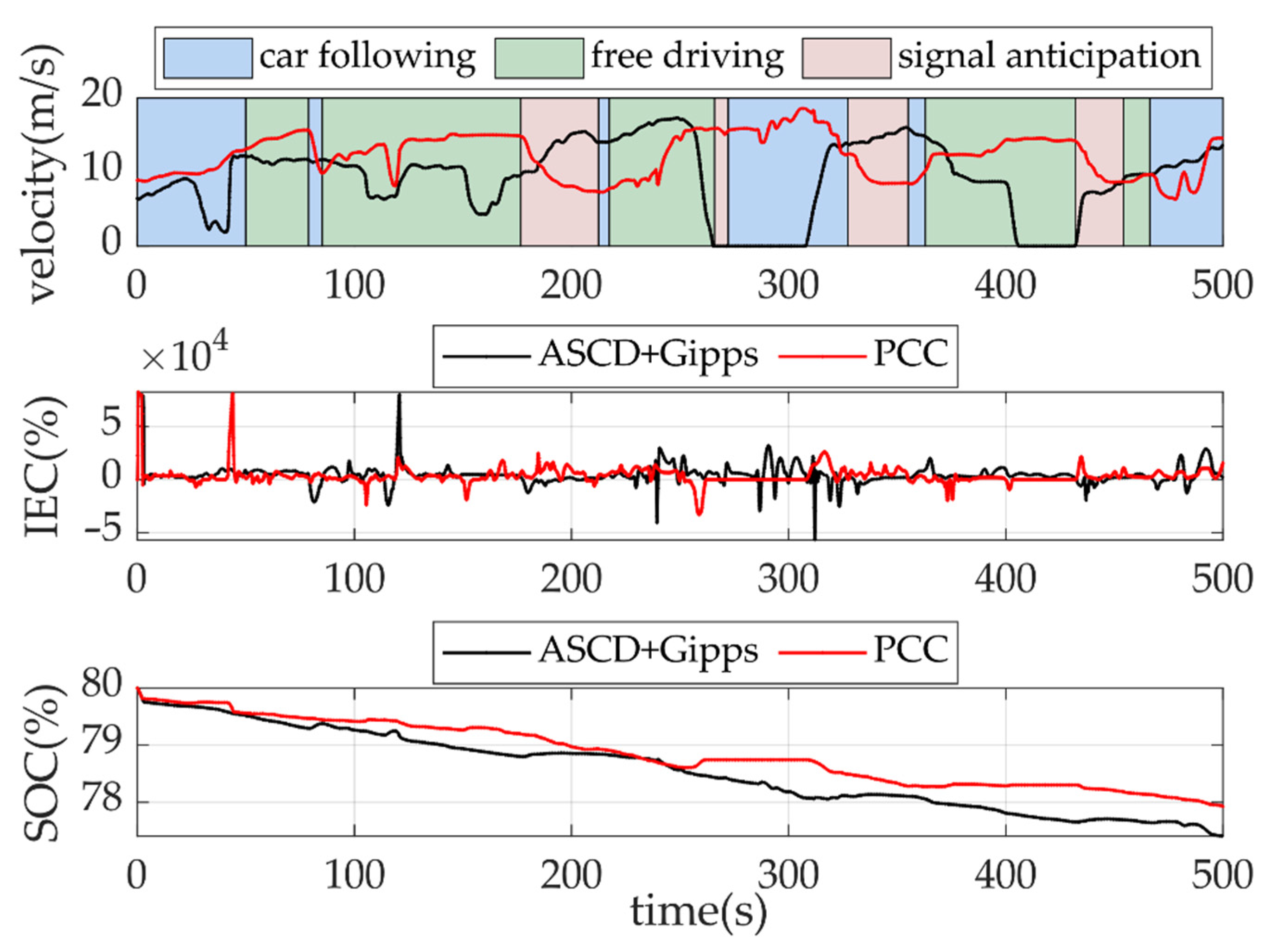
To test the capability of handling the synthetic daily driving scenarios, including all of the above three typical driving scenarios, an area near Kyushu University in Fukuoka, Japan was selected to conduct the comprehensive simulation. The initial velocity of the PCC-vehicle was set as 8.9 . The baseline vehicle was simulated by the automatic speed control drive (ASCD) with Gipps model for car-following. Except for initial velocity, other initial conditions for the baseline vehicle were the same as the PCC-vehicle. Given different control styles, the PCC-vehicle and ASCD-Gipps vehicle faced different traffic situations. The proposed PCC system controlled the vehicle based on the designed eco-driving algorithm, which leads to a relatively conservative driving style while dealing with the car-following scenario, signal anticipation scenario, and free driving scenario. However, the ASCD-Gipps vehicle was controlled by aggressive control actions, imitating the style of a human driver. The detailed description of the Gipps model can be referred to in the book Traffic Flow Dynamics—Data, Models, and Simulation by Martin Treiber and Arne Kesting [39]. The roadmap for the selected area and the simulated synthetic driving scenario is shown in Figure 21.
As shown in Figure 22, the first plot shows the velocity comparison between the PCC-vehicle and baseline ASCD+Gipps-vehicle. The region with different colors represents that the PCC system dynamically switched into driving scenarios, with red representing the signal anticipation scenario, green for the free driving scenario, and blue for the car-following scenario. Within the beginning 50 s, the baseline vehicle first accelerated under the control of ASCD. Then, under the manipulation of the Gipps model, it sharply decelerated to follow the preceding vehicle, while the PCC-vehicle could steadily follow the preceding vehicle without aggressive maneuvers. In the first free driving period, the PCC-vehicle was capable of adjusting its velocity to the desired velocity of 15 based on the road slope information. In the first signal anticipation period, the PCC-vehicle started automatically following the optimal reference velocity to avoid stopping in the upcoming traffic signalized intersection. By contrast, the baseline vehicle was still under acceleration. It turned out that during 260 to 310 s, the PCC-vehicle can pass the intersection without any stop, but the baseline vehicle implemented a stop during the red interval. The same results happened during 406 s to 430 s. The battery SOC percentages for baseline and PCC vehicles are 77.4% and 78.0%, respectively. The cumulative 19.97% energy savings can be achieved.
5. Conclusions
In this research, a tri-level model predictive control (MPC)-based predictive cruise control (PCC) system for electric vehicle (EV) eco-driving is proposed that can be adapted to the urban transport system with synthetic driving scenarios, including car-following, signal anticipation, and free driving scenarios. A co-simulation platform based on CarSim and MATLAB/Simulink was established to validate the effectiveness of the proposed PCC system. Not only the driving comfortability and safety, but the considerable energy-saving rates were also achieved at 16.7%, 12.5%, and 30.3% for three typical driving scenarios, respectively. Finally, a synthetic driving scenario was simulated to test the comprehensive performance of handling the mixed driving scenarios of the proposed PCC system; the simulation results indicated that 19.97% cumulative energy savings was obtained by using the proposed PCC system. The role of MPC in developing an eco-driving strategy for EVs can be justified in the following ways: At first, it can explicitly deal with various state-space variables, especially inequality constraints, which ensures the realization of driving safety and comfortability. Second, MPC features optimization-based control, realizing open-loop optimization and closed-loop control, which guarantees the requirement of energy economy. The proposed PCC system was currently solely tested based on the co-simulation platform using CarSim and MATLAB/Simulink. As a next step, a hardware-in-loop test can be implemented further to test the feasibility of the proposed algorithm and models.
Author Contributions
Conceptualization and methodology, Z.N. and H.F.; investigation, Z.N.; writing, Z.N.; review, editing, and supervising, H.F. Both authors have read and agreed to the published version of the manuscript.
Funding
This research was supported by the Kyushu Natural Energy Promotion Organization, Japan.
Institutional Review Board Statement
Not applicable.
Informed Consent Statement
Not applicable.
Data Availability Statement
Not applicable.
Conflicts of Interest
The authors declare no conflict of interest.
Nomenclature
| EVs | Electric vehicles | - |
| MPC | Model predictive control | - |
| LMPC | Linear model predictive control | - |
| NLMPC | Nonlinear model predictive control | - |
| PCC | Predictive cruise control | - |
| DSSL | Driving scenario switching logic | - |
| SPnT | Signal phase and timing information | - |
| CAVs | Connected and autonomous vehicles | - |
| ITS | Intelligent transport system | - |
| ANN | Artificial neural network | - |
| IECM | Instantaneous energy consumption model | - |
| V2V | Vehicle-to-Vehicle | - |
| V2I | Vehicle-to-Infrastructure | - |
| The relative distance between the host and the preceding vehicle in the same lane | ||
| The real-time driving speed of the preceding vehicle | ||
| The distance to the upcoming signalized intersection | ||
| Allowable speed limitation on a given road section | ||
| Road altitude at a given position | ||
| The traffic signal lights state, including Green, Red, and Yellow | - | |
| The time left for the traffic light of the upcoming intersection | ||
| Braking distance | ||
| Minimum critical distance | ||
| Host vehicle velocity | ||
| Reaction time before braking | ||
| Deceleration during braking | ||
| Thresholds value for the distance to an upcoming signalized intersection | ||
| Thresholds value for the relative distance between the host and preceding vehicles in the same lane | ||
| Real-time estimated time length to pass the upcoming signalized intersection | ||
| Maximum physical allowable acceleration of the vehicle | ||
| Measured state values of the controlled vehicle | - | |
| Measured control values of the controlled vehicle | - | |
| Prediction state values | - | |
| Prediction control values | - | |
| , | Errors between measured values and prediction values | - |
| Electric motor efficiency | - | |
| Motor torque | ||
| Motor speed | ||
| Motor power | ||
| Equivalent internal resistance of the battery | ||
| Equivalent current in the circuit of the battery | ||
| Battery open-circuit voltage | ||
| SOC | Battery state of charge | % |
| Maximum battery capacity | ||
| Vehicle traction force | ||
| Battery maximum power | ||
| Air density | ||
| Aerodynamic drag coefficient | - | |
| Rolling resistance coefficient | - | |
| Frontal area of the vehicle | ||
| Effective radius of the vehicle wheel | ||
| Total mechanical efficiency of the driveline | - | |
| Gear ratio | - | |
| Equivalent total mass of the electric vehicle | ||
| Road gradient | ° | |
| Relative velocity between the host and preceding vehicle | ||
| Safe inter-distance between the host and preceding vehicle | ||
| Actual inter-distance between the host and preceding vehicle | ||
| Error of inter-vehicle distance | ||
| VTH | Variable time headway | - |
| Acceleration of the preceding vehicle | ||
| Acceleration of the host vehicle | ||
| System gain | - | |
| Time constant | ||
| Actual acceleration of the host vehicle | ||
| Optimal desired acceleration of the host vehicle | ||
| , | Start time of the th red and green interval of the upcoming traffic signal light | |
| Reference velocity optimized in signal anticipation scenario | ||
| Instantaneous energy consumption per 0.1 s | ||
| Jerk | ||
| Performance index of the energy economy | - | |
| Weight coefficient of desired acceleration | - | |
| Weight coefficient of the desired jerk | - | |
| Real-time safe distance | ||
| Time-to-collision | ||
| Performance index of driving safety | - | |
| Weight coefficient of the tracking distance error | - | |
| Weight coefficient of the relative velocity | - | |
| , | The lower and upper boundary of inter-distance error | |
| , | The extreme value of relative velocity | |
| , | Driver’s sensitivity to the and | - |
| , | The desired acceleration boundary condition | |
| , | The desired jerk boundary condition | |
| Performance index of driving comfortability | - | |
| Weight coefficient of the host vehicle longitudinal acceleration | - | |
| System cost function under car-following scenario | - | |
| System cost function under signal anticipation scenario | - | |
| Control input | ||
| Prediction horizon | ||
| Weight for the energy consumption under signal anticipation scenario | - | |
| Weight for tracking the reference velocity under signal anticipation | - | |
| Slack factor | - | |
| SQP | Sequential quadratic programming | - |
| Weight for tracking the desired velocity under free driving scenario | - | |
| Weight for acceleration command to avoid hard input because of tracking the desired velocity | - | |
| System cost function under free driving scenario | - | |
| ASCD | Automatic speed control drive | - |
Appendix A
To validate the accuracy of the proposed ANN-based IECM, a multivariate fitting energy consumption model for electric vehicles (EV-MFECM) from reference [40] is compared to show the estimation improvement of ANN-based IECM. EV-MFECM, based on the method of “steady-state estimation + transient correction”, consists of two modules.
From Table A1, the comparative result shows that, under a standard Highway Drive Cycle, both the and values of proposed ANN-based IECM are lower than the corresponding values of baseline EV-MFECM, which indicates that estimation performance of ANN-based IECM is superior to the one based on statistical multivariate regression method. From Figure A1, it is easy to see that both ANN-based IECM and EV-MFECM are capable of reflecting the trend of energy consumption under the Highway Drive Cycle. However, it is evident that the proposed ANN-based IECM fits better and is more accurate than the baseline. The error of ANN-based IECM is closer to zero without any spikes. Besides, the EV-MFECM contains the polynomial combination, which makes it too complicated to be deployed in real applications. On the contrary, ANN-based IECM features an explicit model structure and is easy to encode into the hardware, making it more suitable for vehicle eco-driving optimization systems.

Table A1.
The comparative validation result of ANN-ICEM.
| ANN-based IECM | 1.25 | |
| EV-MFECM | 3.20 |
Figure A1.
Comparison of estimation of models with actual value and estimation error of different models.
Figure A1.
Comparison of estimation of models with actual value and estimation error of different models.

References
- Alshehry, A.S.; Belloumi, M. Study of the environmental Kuznets curve for transport carbon dioxide emissions in Saudi Arabia. Renew. Sustain. Energy Rev. 2017, 75, 1339–1347. [Google Scholar] [CrossRef]
- NeV. Strategy for Diffusing the Next Generation Vehicles in Japan; Next Generation Vehicle Promotion Center: Tokyo, Japan, 2018. [Google Scholar]
- METI. Japan’s Energy 2020; Agency for Natural Resources and Energy: Tokyo, Japan, 2020.
- Motoko, H. Japan’s EV Shift to Boost Power Demand by 15pc: IEEJ; Commodity & Energy Price Benchmarks|Argus Media: Tokyo, Japan, 2021. [Google Scholar]
- Zhou, M.; Hui, J.; Wenshuo, W. A review of vehicle fuel consumption models to evaluate eco-driving and eco-routing. Transp. Res. Part D Transp. Environ. 2016, 49, 203–218. [Google Scholar] [CrossRef]
- Li, M.; Wu, X.; He, X.; Yu, G.; Wang, Y. An eco-driving system for electric vehicles with signal control under V2X environment. Transp. Res. Part C Emerg. Technol. 2018, 93, 335–350. [Google Scholar] [CrossRef]
- Maamria, D.; Gillet, K.; Colin, G.; Chamaillard, Y.; Nouillant, C. Optimal predictive eco-driving cycles for conventional, electric, and hybrid electric cars. IEEE Trans. Veh. Technol. 2019, 68, 6320–6330. [Google Scholar] [CrossRef] [Green Version]
- Cheng, Q.; Nouveliére, L.; Orfila, O. A New Eco-driving Assistance System for a Light Vehicle: Energy Management and Speed Optimization. In Proceedings of the IEEE Intelligent Vehicles Symposium, Gold Coast, Australia, 23–26 June 2013; pp. 1434–1439. [Google Scholar]
- Gáspár, P.; Németh, B. Predictive Cruise Control for Road Vehicles Using Road and Traffic Information; Springer: Berlin/Heidelberg, Germany, 2018. [Google Scholar]
- Lattemann, F.; Neiss, K.; Terwen, S.; Connolly, T. The predictive cruise control—A system to reduce fuel consumption of heavy-duty trucks. SAE Tech. Pap. Ser. 2004, 113, 139–146. [Google Scholar]
- Hellström, E.; Ivarsson, M.; Åslund, J.; Nielsen, L. Look-ahead control for heavy trucks to minimize trip time and fuel consumption. Control Eng. Pract. 2009, 17, 245–254. [Google Scholar] [CrossRef] [Green Version]
- Hellström, E. Explicit Use of Road Topography for Model Predictive Cruise Control in Heavy Trucks. Master’s Thesis, Linköping University, Linköping, Sweden, 2005. [Google Scholar]
- Hellström, E. Look-Ahead Control of Heavy Trucks Utilizing Road Topography. Ph.D. Thesis, Linköping University, Linköping, Sweden, 2007. [Google Scholar]
- Hellström, E.; Fröberg, A.; Nielsen, L. A real-time fuel-optimal cruise controller for heavy trucks using road topography information. SAE Tech. Pap. Ser. 2006. [Google Scholar] [CrossRef]
- Hellström, E.; Åslund, J.; Nielsen, L. Design of an efficient algorithm for fuel-optimal look-ahead control. Control Eng. Pract. 2010, 18, 1318–1327. [Google Scholar] [CrossRef] [Green Version]
- Kamal, M.A.; Mukai, M.; Murata, J.; Kawabe, T. Ecological vehicle control on roads with up-down slopes. IEEE Trans. Intell. Transp. Syst. 2011, 12, 783–794. [Google Scholar] [CrossRef]
- Yu, Q. Vehicular Speed Control of Eco-Driving Systems Based on Connected Vehicles. Master’s Thesis, Tsinghua University, Beijing, China, 2014. [Google Scholar]
- Markschläger, P.; Wahl, H.; Weberbauer, F.; Lederer, M. Assistance system for higher fuel efficiency. ATZ Worldw. 2012, 114, 8–13. [Google Scholar] [CrossRef]
- Asadi, B.; Vahidi, A. Predictive cruise control: Utilizing upcoming traffic signal information for improving fuel economy and reducing trip time. IEEE Trans. Control Syst. Technol. 2011, 19, 707–714. [Google Scholar] [CrossRef]
- Kamal, M.A.; Mukai, M.; Murata, J.; Kawabe, T. Model predictive control of vehicles on urban roads for improved fuel economy. IEEE Trans. Control Syst. Technol. 2013, 21, 831–841. [Google Scholar] [CrossRef]
- De Nunzio, G.; De Wit, C.C.; Moulin, P.; Di Domenico, D. Eco-driving in urban traffic networks using traffic signals information. Int. J. Robust Nonlinear Control 2015, 26, 1307–1324. [Google Scholar] [CrossRef] [Green Version]
- Meng, X.; Cassandras, C.G. A real-time optimal eco-driving approach for autonomous vehicles crossing multiple signalized intersections. In Proceedings of the 2019 American Control Conference (ACC), Philadelphia, PA, USA, 10–12 July 2019. [Google Scholar]
- Bae, S.; Kim, Y.; Guanetti, J.; Borrelli, F.; Moura, S. Design and implementation of ecological adaptive cruise control for autonomous driving with communication to traffic lights. In Proceedings of the 2019 American Control Conference (ACC), Philadelphia, PA, USA, 10–12 July 2019. [Google Scholar]
- Zhang, J.; Ioannou, P. Longitudinal control of heavy trucks in mixed traffic: Environmental and fuel economy considerations. IEEE Trans. Intell. Transp. Syst. 2006, 7, 92–104. [Google Scholar] [CrossRef]
- Li, S.; Li, K.; Wang, J.; Zhang, L.; Lian, X.; Hiroshi, U.; Bai, D. MPC based vehicular following control considering both fuel economy and tracking capability. In Proceedings of the 2008 IEEE Vehicle Power and Propulsion Conference, Harbin, China, 3–5 September 2008. [Google Scholar]
- Bakibillah, A.S.M.; Kamal, M.A.S.; Tan, C.P.; Hayakawa, T.; Imura, J. Eco-driving on Hilly Roads Using Model Predictive Control. In Proceedings of the 2018 Joint 7th International Conference on Informatics, Electronics & Vision (ICIEV) and 2018 2nd International Conference on Imaging, Vision & Pattern Recognition (icIVPR), Kitakyushu, Japan, 25–29 June 2018. [Google Scholar] [CrossRef]
- Ma, F.; Yang, Y.; Wang, J.; Liu, Z.; Li, J.; Nie, J.; Shen, Y.; Wu, L. Predictive energy-saving optimization based on nonlinear model predictive control for cooperative connected vehicles platoon with V2V communication. Energy 2019, 189, 116120. [Google Scholar] [CrossRef]
- Nie, Z.; Farzaneh, H. Adaptive Cruise Control for Eco-Driving Based on Model Predictive Control Algorithm. Appl. Sci. 2020, 10, 5271. [Google Scholar] [CrossRef]
- Hu, X.; Zhang, X.; Tang, X.; Lin, X. Model predictive control of hybrid electric vehicles for fuel economy, emission reductions, and inter-vehicle safety in car-following scenarios. Energy 2020, 196, 117101. [Google Scholar] [CrossRef]
- Yang, C.; Wang, M.; Wang, W.; Pu, Z.; Ma, M. An efficient vehicle-following predictive energy management strategy for PHEV based on improved sequential quadratic programming algorithm. Energy 2021, 219, 119595. [Google Scholar] [CrossRef]
- Manzie, C.; Watson, H.; Halgamuge, S. Fuel economy improvements for urban driving: Hybrid vs. intelligent vehicles. Transp. Res. Part C Emerg. Technol. 2007, 15, 1–16. [Google Scholar] [CrossRef]
- Li, S.E.; Peng, H.; Li, K.; Wang, J. Minimum fuel control strategy in automated car-following scenarios. IEEE Trans. Veh. Technol. 2012, 61, 998–1007. [Google Scholar] [CrossRef]
- Li, L.; Wang, X.; Song, J. Fuel consumption optimization for smart hybrid electric vehicle during a car-following process. Mech. Syst. Signal Process. 2017, 87, 17–29. [Google Scholar] [CrossRef]
- Su, L.H.; Li, L.; Chu, J. Recent Advances on Predictive Control. Mech. Electr. Eng. Mag. 2011, 5, 4–8. [Google Scholar]
- Yi, C.; Epureanu, B.I.; Hong, S.; Ge, T.; Yang, X.G. Modeling, control, and performance of a novel architecture of hybrid electric powertrain system. Appl. Energy 2016, 178, 454–467. [Google Scholar] [CrossRef]
- Sun, C.; Moura, S.J.; Hu, X.; Hedrick, J.K.; Sun, F. Dynamic traffic feedback data enabled energy management in plug-in hybrid electric vehicles. IEEE Trans. Control Syst. Technol. 2015, 23, 1075–1086. [Google Scholar]
- Li, S. Vehicular Multi-Objective Coordinated Adaptive Cruise Control. Ph.D. Thesis, Tsinghua University, Beijing, China, 2009. [Google Scholar]
- Marquardt, D. An Algorithm for Least-Squares Estimation of Nonlinear Parameters. J. Soc. Ind. Appl. Math. 1963, 11, 431–441. [Google Scholar] [CrossRef]
- Treiber, M.; Kesting, A. Traffic Flow Dynamics: Data, Models and Simulation; Springer Science & Business Media: Berlin, Germany, 2012. [Google Scholar]
- Yu, Y.; Li, Y.; Liang, Y.; Zhang, Z.; Liao, G. Modeling of Transient Energy Consumption Model of Electric Vehicle Based on Data Mining. In Proceedings of the Society of Automotive Engineers of Automotive Engineering Conference, Shanghai, China, 21–22 May 2019; pp. 277–283. [Google Scholar]
Figure 1.
Schematic of predictive cruise control system for EV eco-driving.

Figure 2.
Flow chart for driving scenario switching logic (DSSL).

Figure 3.
Three typical driving scenarios of PCC system architecture based on MPC algorithm.

Figure 4.
Diagram of inputs and output for ANN-based IECM.

Figure 5.
MPC controller structure in the car-following scenario.

Figure 6.
Fundamental concept of the signal anticipation scenario.

Figure 7.
Workflow of the MPC problem for the signal anticipation scenario.

Figure 8.
Basic concept of the free driving scenario.

Figure 9.
Workflow of the MPC problem for the free driving scenario.

Figure 10.
Parametric modeling of vehicle dynamics within CarSim.

Figure 11.
Visualization of free driving scenario (left), car-following scenario (middle), and signal anticipation scenario (right).
Figure 11.
Visualization of free driving scenario (left), car-following scenario (middle), and signal anticipation scenario (right).

Figure 12.
(a) Simulation platform for car-following scenario, (b) simulation platform for signal anticipation scenario, (c) simulation platform for free driving scenario.
Figure 12.
(a) Simulation platform for car-following scenario, (b) simulation platform for signal anticipation scenario, (c) simulation platform for free driving scenario.


Figure 13.
Flow chart of real-world data acquisition and transmission.

Figure 14.
Simulation visualization of a steady following scene.

Figure 15.
Simulation results of the steady car-following scenario.

Figure 16.
Roadmap for the signal anticipation scenario.

Figure 17.
Simulation results and space-time diagram with SPnT information comparing preceding and host vehicles with PCC system during low traffic flow and high traffic flow.
Figure 17.
Simulation results and space-time diagram with SPnT information comparing preceding and host vehicles with PCC system during low traffic flow and high traffic flow.

Figure 18.
Simulation visualization for the free driving scenario.

Figure 19.
Global coordinate of hilly road section.

Figure 20.
Simulation results for the free driving scenario.

Figure 21.
Roadmap of the selected area and the simulated synthetic driving scenario.

Figure 22.
Simulation results for the synthetic driving scenario.

Table 1.
V2V and V2I data interaction in this research.
| Data | Explanation | Unit |
|---|---|---|
| The relative distance between the host and the preceding vehicle in the same lane | ||
| The real-time driving speed of the preceding vehicle | ||
| The distance to the upcoming signalized intersection | ||
| Allowable speed limitation on a given road section | ||
| Road altitude at a given position | ||
| The traffic signal lights state, including Green, Red, Yellow | - | |
| The time left for the traffic light of the upcoming intersection |
Table 2.
Specifications of the electric vehicle longitudinal dynamics model.
| Specification | Values |
|---|---|
| Equivalent total mass of the electric vehicle, | 1260 |
| Gear ratio, | 3.905 |
| Total mechanical efficiency of the driveline, | 0.95 |
| Effective radius of the vehicle wheel, | 287 |
| Frontal area of the vehicle, | 2.22 |
| Rolling resistance coefficient, | 0.028 |
| Aerodynamic drag coefficient, | 0.316 |
| Air density, | 1.206 |
| Motor | Maximum available power: = 55; Maximum output torque: 305; |
| Battery | Battery voltage: 6~9 V; Packs: 40; Initial charge level: 0.8; : 93 Ah |
Table 3.
Simulation parameters.
| Parameter | Symbol | Values & Unit |
|---|---|---|
| System gain | 1.05 | |
| Time constant | 0.40 s | |
| Minimal stop distance | 5 m | |
| Sampling period | 0.1 s | |
| Prediction horizon | 30 | |
| Time-to-collision | −2.5 s | |
| Sensitivity first-order term coefficient of | 0.06 | |
| Sensitivity first-order term coefficient of | 0.005 | |
| Constant term of sensitivity of | −0.13 | |
| Constant term of sensitivity of | 0.92 | |
| Upper bound of acceleration | 1.5 m/s2 | |
| Lower bound of acceleration | −2 m/s2 | |
| Upper bound of jerk | () | 1.5 m/s3 |
| Lower bound of jerk | () | 2 m/s3 |
Publisher’s Note: MDPI stays neutral with regard to jurisdictional claims in published maps and institutional affiliations. |
© 2021 by the authors. Licensee MDPI, Basel, Switzerland. This article is an open access article distributed under the terms and conditions of the Creative Commons Attribution (CC BY) license (https://creativecommons.org/licenses/by/4.0/).
Share and Cite
MDPI and ACS Style
Nie, Z.; Farzaneh, H. Role of Model Predictive Control for Enhancing Eco-Driving of Electric Vehicles in Urban Transport System of Japan. Sustainability 2021, 13, 9173. https://0-doi-org.brum.beds.ac.uk/10.3390/su13169173
AMA Style
Nie Z, Farzaneh H. Role of Model Predictive Control for Enhancing Eco-Driving of Electric Vehicles in Urban Transport System of Japan. Sustainability. 2021; 13(16):9173. https://0-doi-org.brum.beds.ac.uk/10.3390/su13169173
Chicago/Turabian StyleNie, Zifei, and Hooman Farzaneh. 2021. "Role of Model Predictive Control for Enhancing Eco-Driving of Electric Vehicles in Urban Transport System of Japan" Sustainability 13, no. 16: 9173. https://0-doi-org.brum.beds.ac.uk/10.3390/su13169173
Note that from the first issue of 2016, this journal uses article numbers instead of page numbers. See further details here.