
Built Environment Typologies Prone to Risk: A Cluster Analysis of Open Spaces in Italian Cities

 , , , , and
Abstract
:1. Introduction
1.1. Built Environment and Multi-Risk Approach
1.2. Towards the Idealization of the Built Environment
1.3. Work Aims and Research Approach
2. Materials and Methods
2.1. Open Space Parameters for BET Definition
- Parameters for a fast analysis (morphological, geometric, and functional characteristics): P1, P2, P4, P5, P8, and P9;
- Parameters for a detailed analysis (constructive characteristics): P3, P6, and P7.
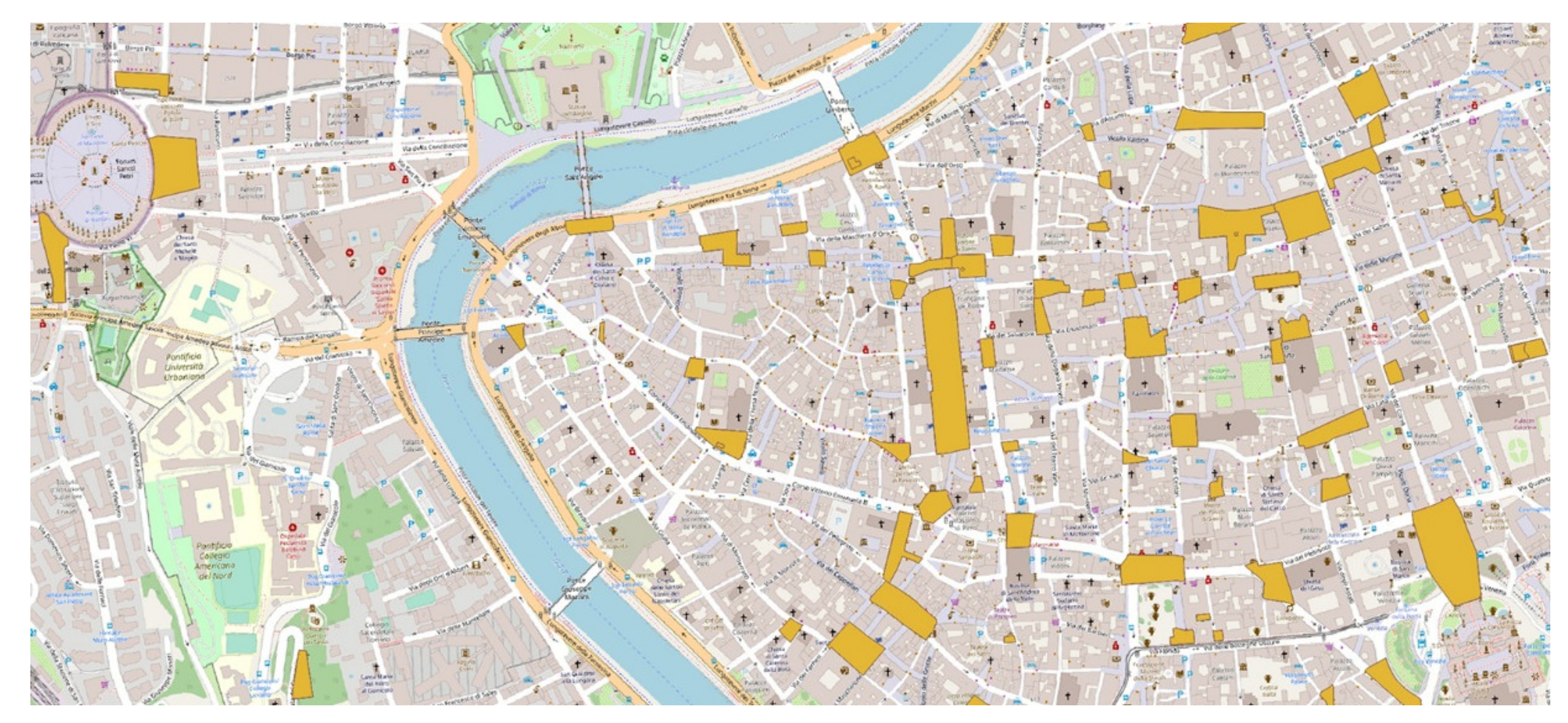
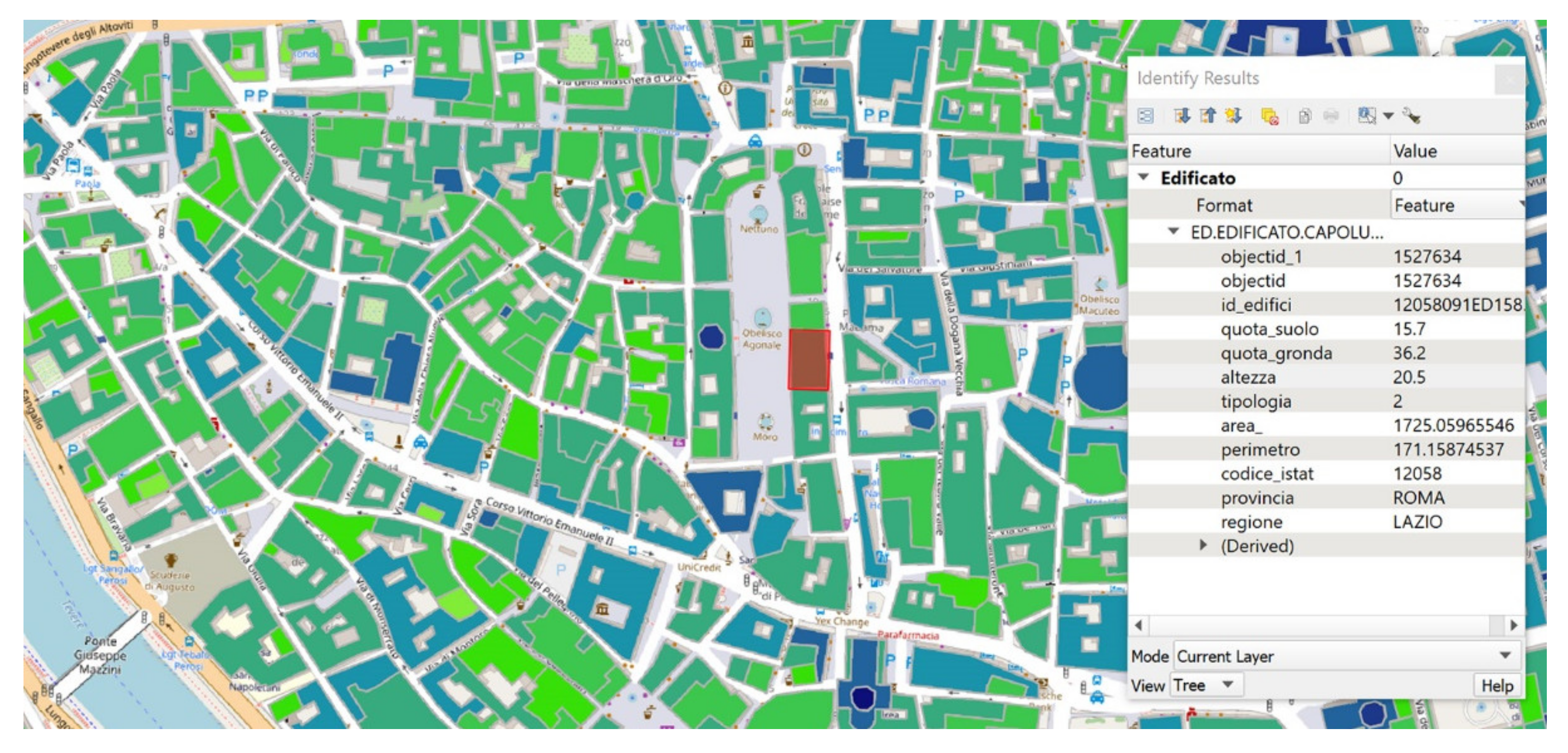
2.2. GIS Databases and Parameter Extraction
- Minimum oriented bounding box—to calculate the rotated rectangle of the minimum area that covers each OS, to extract its area (AMOBB);
- Minimum circumscribed circumference—to calculate the minimum circumscribed circumference that covers each OS, to extract its diameter (d1) and radius (r1);
- Inaccessibility pole—to find the centre of the maximum inscribed circumference for each OS, to extract its diameter (d2) and radius (r2);
- Buffer—to create a buffer area for all elements in an input vector, using a fixed or dynamic distance.
- Merge—to combine multiple vector layers having the same type of geometry into a single vector;
- Intersection—to extract the parts of the overlapping elements in the input and overlap layers. The overlapping geometry attributes from both the input and overlay layers are assigned to the elements of the output intersection layer;
- Fix geometry—to create a valid representation of a given invalid geometry without losing any of the starting vertices;
- Join attributes by locations—to create a new vector with additional attributes added to the attribute table. The additional attributes and their values are taken from a second vector. A spatial criterion is applied to select the values from the second vector that are added to each element of the first vector and are part of the result.
- AAS is the area of the considered OS, and
- AMOBB is the area of the minimum oriented bounding box of the considered OS.
- r2 is the radius of the maximum inscribed circumference, calculated through the inaccessibility pole; and
- r1 is the radius of the minimum circumscribed circumference.
- Hmax is the maximum height of the buildings that define the OS perimeter, and
- d2 is the diameter of the maximum inscribed circumference.
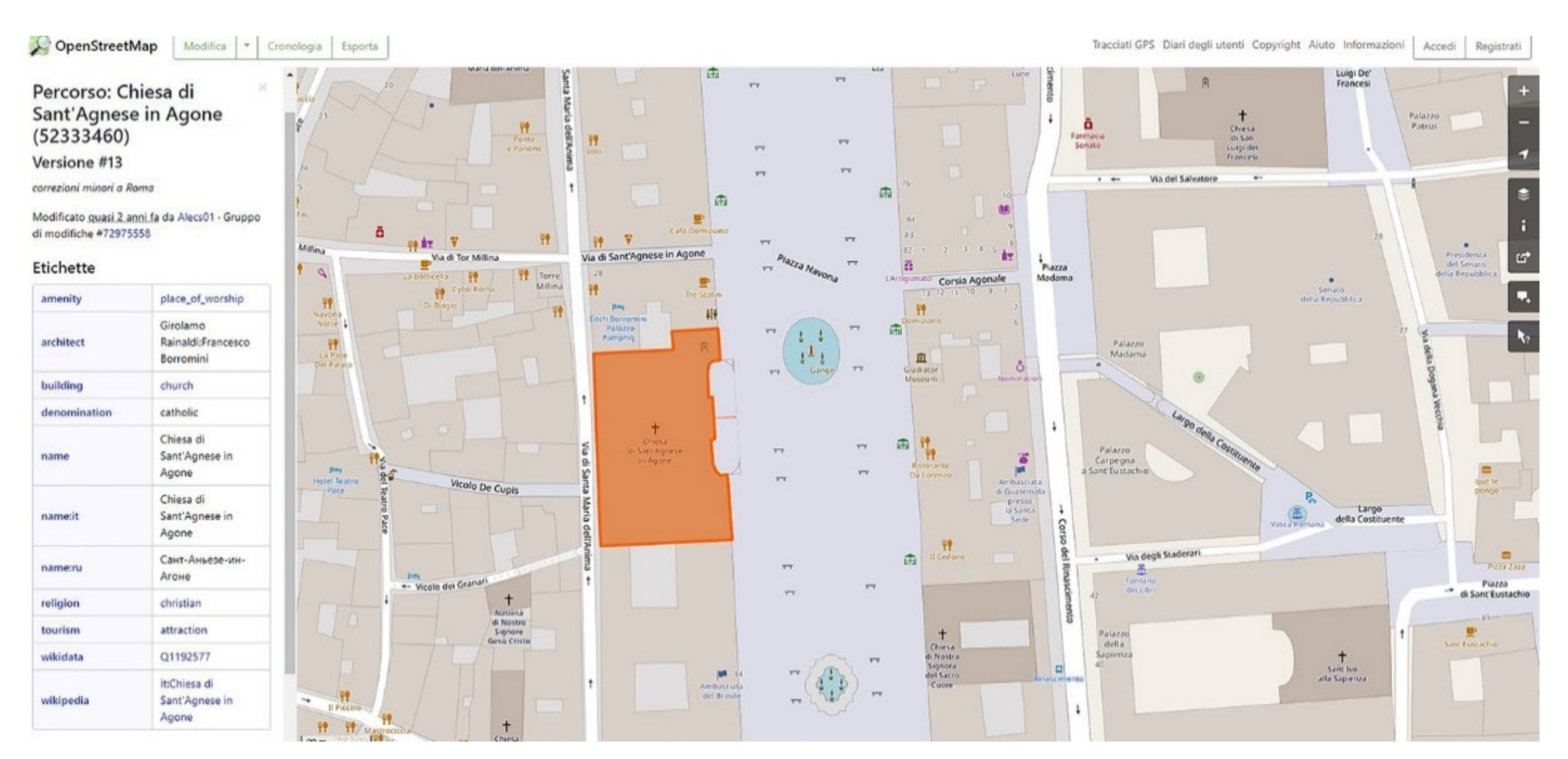
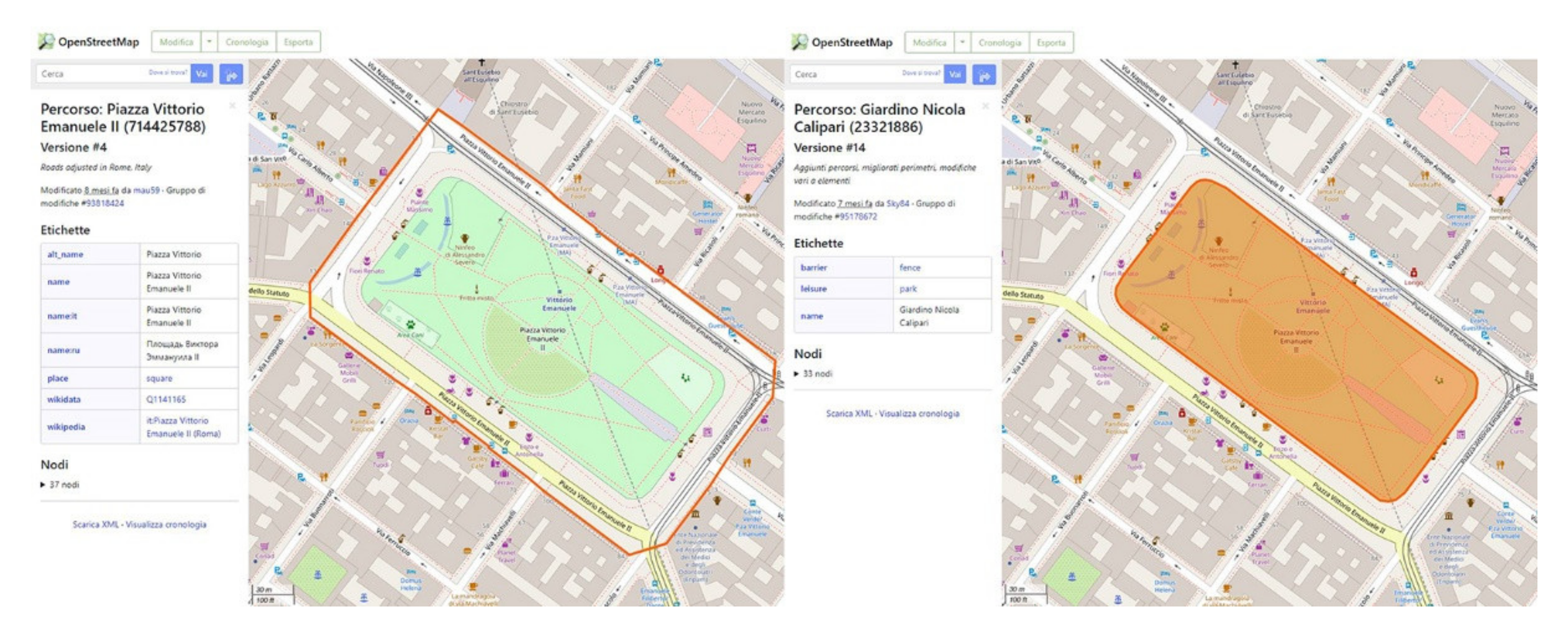
- religious buildings (e.g., churches or other places of worship; Figure 5);
- public buildings (e.g., town halls and police offices);
- buildings for education (e.g., schools, colleges, and universities); and
- buildings with cultural or tourism importance (e.g., museums, palaces, and castles).
2.3. Cluster Analysis
2.4. From Cluster Analysis to BET Identification
3. Results
3.1. Data Set Description
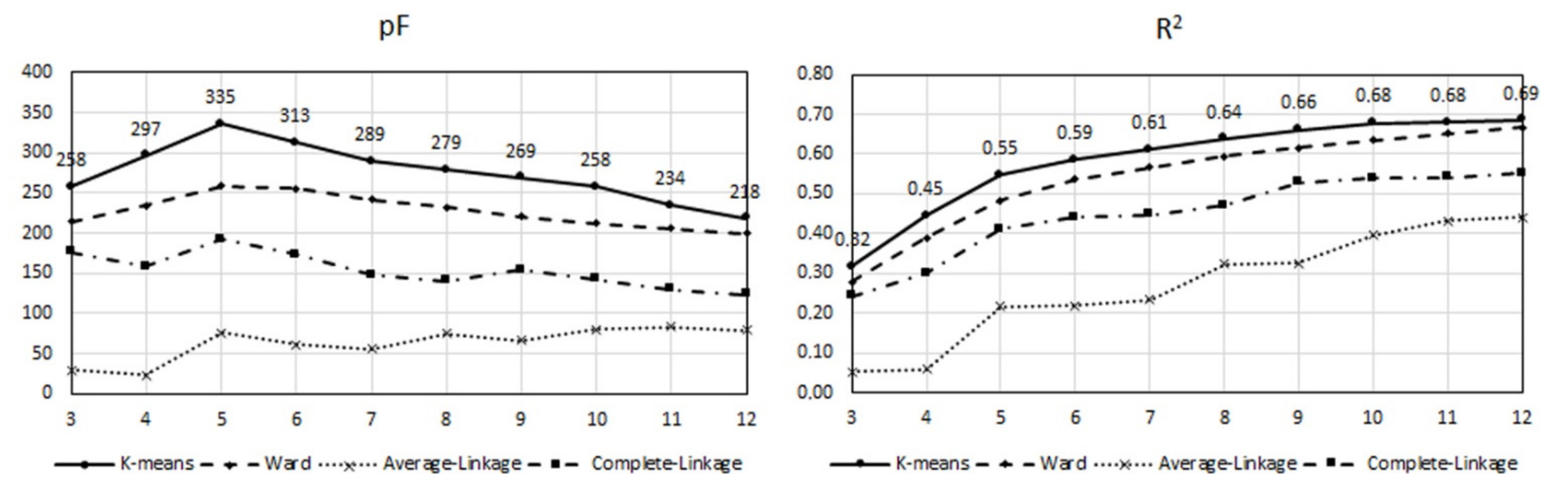
3.2. Cluster Analysis
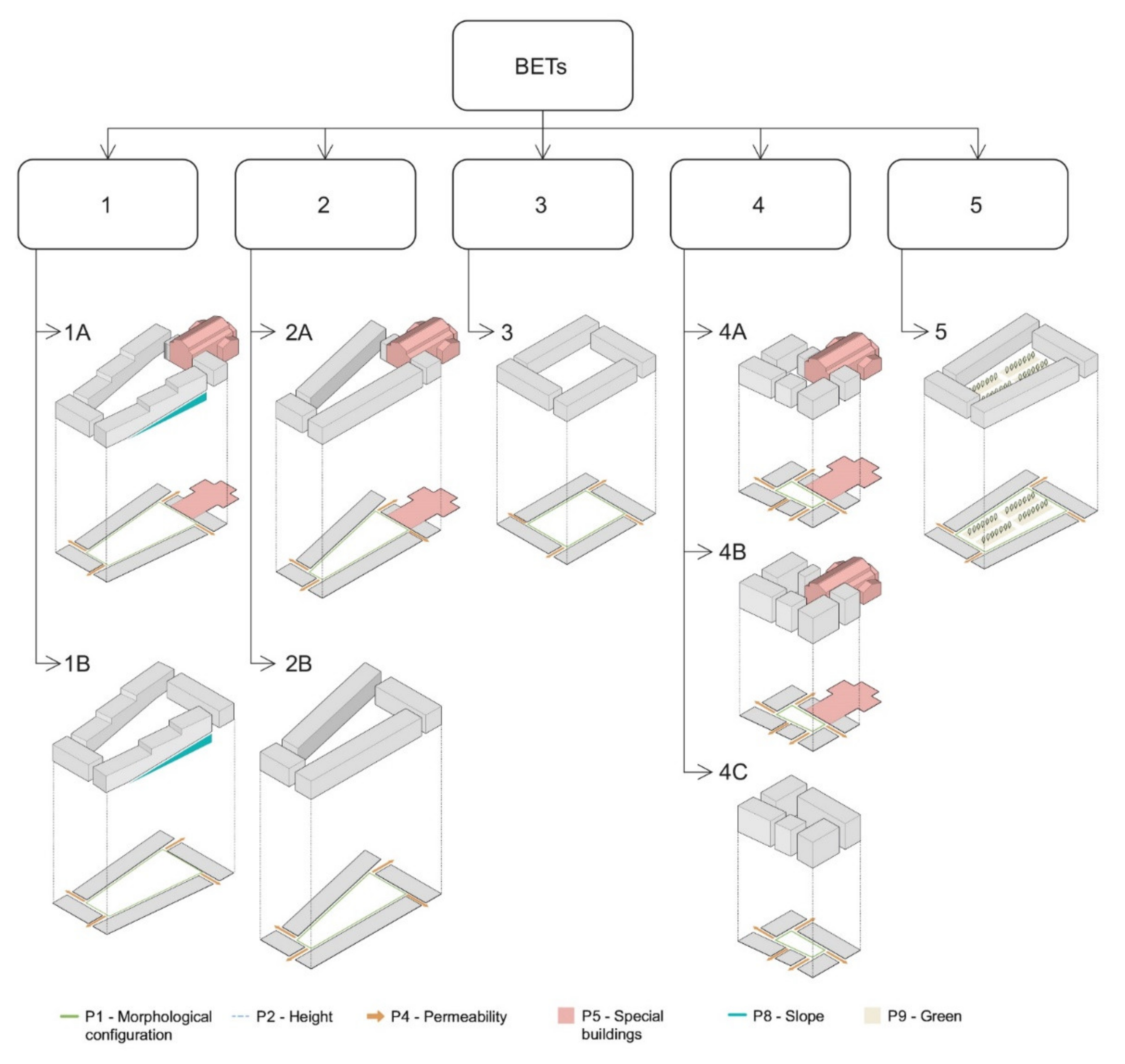
3.3. BET Definition
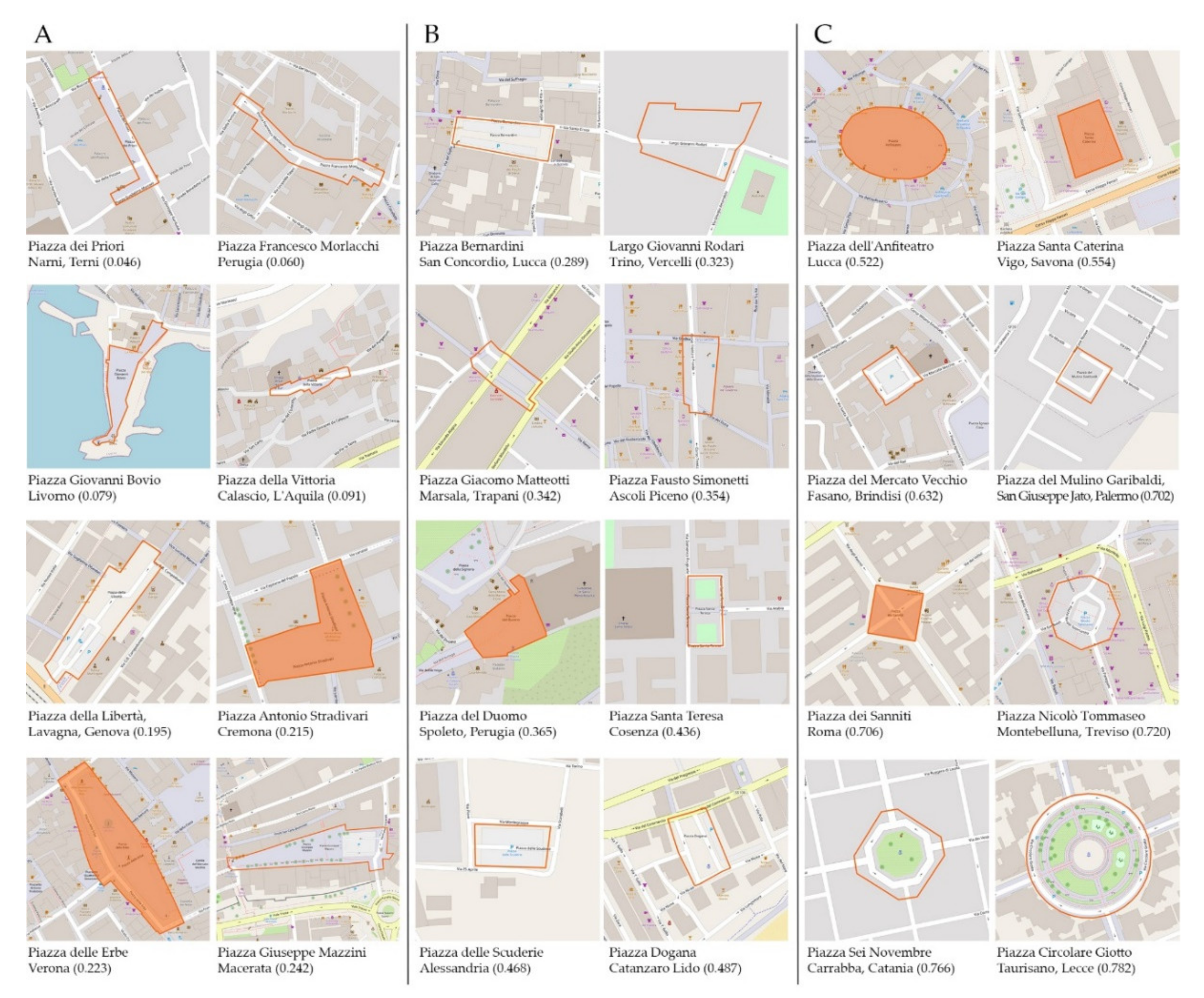
3.4. BET Representation and Real Case Studies
4. Discussion
4.1. From BETs towards Risk Analysis
4.2. Limitations and Advancement in the Research Field
5. Conclusions
Author Contributions
Funding
Institutional Review Board Statement
Informed Consent Statement
Data Availability Statement
Conflicts of Interest
References
- Scolobig, A.; Garcia-aristizabal, A.; Komendantova, N.; Patt, A.; Ruocco, A.D.; Gasparini, P.; Monfort, D.; Vinchon, C.; Mrzy, R.; Fleming, K.; et al. From Multi-Risk Assessment to Multi-Risk Governance: Recommendations for Future Directions. In Understanding Risk: The Evolution of Disaster Risk Assessment; GFDRR, Ed.; International Bank for reconstruction and Development: Washington, DC, USA, 2015; pp. 163–167. [Google Scholar]
- Komendantova, N.; Mrzyglocki, R.; Mignan, A.; Khazai, B.; Wenzel, F.; Patt, A.; Fleming, K. Multi-hazard and multi-risk decision-support tools as a part of participatory risk governance: Feedback from civil protection stakeholders. Int. J. Disaster Risk Reduct. 2014, 8, 50–67. [Google Scholar] [CrossRef] [Green Version]
- Dilley, M.; Chen, R.S.; Deichmann, U.; Lerner-Lam, A.L.; Arnold, M. Natural Disaster Hotspots: A Global Risk Analysis; World Bank: Washington, DC, USA, 2005. [Google Scholar]
- IPCC. Managing the Risks of Extreme Events and Disasters to Advance Climate Change Adaptation; Intergovernmental Panel On Climate Change, Ed.; Cambridge University Press: Cambridge, UK, 2012; Volume 9781107025, ISBN 9781139177245. [Google Scholar]
- WHO. Definitions: Emergencies. Available online: https://www.who.int/hac/about/definitions/en/ (accessed on 29 November 2019).
- PreventionWeb—UNDRR. Available online: https://www.preventionweb.net/terminology#D (accessed on 2 October 2020).
- UNISDR. Sendai Framework for Disaster Risk Reduction 2015–2030; United Nations Office for Disaster Risk Reduction: Geneva, Switzerland, 2015; Available online: http://www.unisdr.org/files/43291_sendaiframeworkfordrren.pdf (accessed on 1 September 2020).
- Kappes, M.S.; Keiler, M.; von Elverfeldt, K.; Glade, T. Challenges of analyzing multi-hazard risk: A review. Nat. Hazards 2012, 64, 1925–1958. [Google Scholar] [CrossRef] [Green Version]
- Gallina, V.; Torresan, S.; Critto, A.; Sperotto, A.; Glade, T.; Marcomini, A. A review of multi-risk methodologies for natural hazards: Consequences and challenges for a climate change impact assessment. J. Environ. Manag. 2016, 168, 123–132. [Google Scholar] [CrossRef]
- Sharifi, A. Urban form resilience: A meso-scale analysis. Cities 2019, 93, 238–252. [Google Scholar] [CrossRef]
- Russo, M.; Angelosanti, M.; Bernardini, G.; Cantatore, E.; D’Amico, A.; Currà, E.; Fatiguso, F.; Mochi, G.; Quagliarini, E. Morphological Systems of Open Spaces in Built Environment Prone to Sudden-Onset Disasters. In Sustainability in Energy and Buildings 2020 (Part of the Smart Innovation, Systems and Technologies Book Series—SIST, Volume 203—ISSN: 2190–3018); Littlewood, J., Howlett, R.J., Jain, L.C., Eds.; Springer: Singapore, 2021; pp. 321–331. ISBN 978-981-15-8783-2. [Google Scholar]
- French, E.L.; Birchall, S.J.; Landman, K.; Brown, R.D. Designing public open space to support seismic resilience: A systematic review. Int. J. Disaster Risk Reduct. 2019, 34, 1–10. [Google Scholar] [CrossRef] [Green Version]
- Arosio, M.; Martina, M.L.V.; Figueiredo, R. The whole is greater than the sum of its parts: A holistic graph-based assessment approach for natural hazard risk of complex systems. Nat. Hazards Earth Syst. Sci. 2020, 20, 521–547. [Google Scholar] [CrossRef] [Green Version]
- Gill, J.C.; Malamud, B.D. Hazard interactions and interaction networks (cascades) within multi-hazard methodologies. Earth Syst. Dyn. 2016, 7, 659–679. [Google Scholar] [CrossRef] [Green Version]
- Mignan, A.; Wiemer, S.; Giardini, D. The quantification of low-probability-high-consequences events: Part I. A generic multi-risk approach. Nat. Hazards 2014, 73, 1999–2022. [Google Scholar] [CrossRef] [Green Version]
- Bernardini, G.; Romano, G.; Soldini, L.; Quagliarini, E. How urban layout and pedestrian evacuation behaviours can influence flood risk assessment in riverine historic built environments. Sustain. Cities Soc. 2021, 70, 102876. [Google Scholar] [CrossRef]
- White, G.F.; Kates, R.W.; Burton, I. Knowing better and losing even more: The use of knowledge in hazards management. Environ. Hazards 2001, 3, 81–92. [Google Scholar] [CrossRef] [Green Version]
- Dunant, A.; Bebbington, M.; Davies, T.; Horton, P. Multihazards Scenario Generator: A Network-Based Simulation of Natural Disasters. Risk Anal. 2021. [Google Scholar] [CrossRef]
- Schmidt, J.; Matcham, I.; Reese, S.; King, A.; Bell, R.; Henderson, R.; Smart, G.; Cousins, J.; Smith, W.; Heron, D. Quantitative multi-risk analysis for natural hazards: A framework for multi-risk modelling. Nat. Hazards 2011, 58, 1169–1192. [Google Scholar] [CrossRef]
- Koren, D.; Rus, K. The potential of open space for enhancing urban seismic resilience: A literature review. Sustainability 2019, 11, 5942. [Google Scholar] [CrossRef] [Green Version]
- Russo, M.; Angelosanti, M.; Bernardini, G.; Cantatore, E.; D’Amico, A.; Currà, E.; Fatiguso, F.; Mochi, G.; Quagliarini, E. Morphological systems of open spaces in built environment prone to Sudden-onset disasters. In Proceedings of the International Conference on Sustainability in Energy and Buildings SEB 2020, Split, Croatia, 24–26 June 2020; pp. 1–10. [Google Scholar]
- Quagliarini, E.; Lucesoli, M.; Bernardini, G. How to create seismic risk scenarios in historic built environment using rapid data collection and managing. J. Cult. Herit. 2021, 48, 93–105. [Google Scholar] [CrossRef]
- Mandolesi, E.; Ferrero, A. Piazze del Piceno; Gangemi: Rome, Italy, 2001; ISBN 9788849201307. [Google Scholar]
- Zuccaro, G.; Dolce, M.; De Gregorio, D.; Speranza, E.; Moroni, C. La Scheda Cartis Per La Caratterizzazione Tipologico- Strutturale Dei Comparti Urbani Costituiti Da Edifici Ordinari. Valutazione dell’esposizione in analisi di rischio sismico. In Proceedings of the 39th National Conference of the National Group of Geophysics of the Solid Earth GNGTS 2015 (Gruppo Nazionale di Geofisica della Terra Solida), Trieste, Italy, 17–19 November 2015; pp. 281–287. [Google Scholar]
- Dolce, M.; Prota, A.; Borzi, B.; da Porto, F.; Lagomarsino, S.; Magenes, G.; Moroni, C.; Penna, A.; Polese, M.; Speranza, E.; et al. Seismic Risk Assessment of Residential Buildings in Italy; Springer: Dordrecht, The Netherlands, 2020; ISBN 0123456789. [Google Scholar]
- Morganti, M.; Salvati, A.; Coch, H.; Cecere, C. Urban morphology indicators for solar energy analysis. Energy Procedia 2017, 134, 1–8. [Google Scholar] [CrossRef]
- Morganti, M. Spatial Metrics to Investigate the Impact of Urban Form on Microclimate and Building Energy Performance: An Essential Overview. In Urban Microclimate Modelling for Comfort and Energy Studies; Palme, M., Salvati, A., Eds.; Springer: Cham, Germany, 2021; pp. 385–402. [Google Scholar]
- Mignot, E.; Li, X.; Dewals, B. Experimental modelling of urban flooding: A review. J. Hydrol. 2019, 568, 334–342. [Google Scholar] [CrossRef] [Green Version]
- Ronchi, E.; Kuligowski, E.D.; Reneke, P.A.; Peacock, R.D.; Nilsson, D. The Process of Verification and Validation of Building Fire Evacuation Models. NIST Tech. Note 2013, 1822, 84. [Google Scholar]
- Lovreglio, R.; Ronchi, E.; Maragkos, G.; Beji, T.; Merci, B. A dynamic approach for the impact of a toxic gas dispersion hazard considering human behaviour and dispersion modelling. J. Hazard. Mater. 2016, 318, 758–771. [Google Scholar] [CrossRef]
- Cimellaro, G.P.; Ozzello, F.; Vallero, A.; Mahin, S.; Shao, B. Simulating earthquake evacuation using human behavior models. Earthq. Eng. Struct. Dyn. 2017, 46, 985–1002. [Google Scholar] [CrossRef]
- BE S2ECURE project D 3.1.1 | BETs Definition and Representation Report; 2021; Working Report (draft) from BE S2ECURe “(make) Built Environment Safer in Slow and Emergency Conditions through BehavioUral Assessed/Designed Resilient Solutions” Research Project. Available online: http://bit.ly/bes2ecure_D311 (accessed on 31 May 2021).
- Tate, N.J.; Fisher, P.F.; Martin, D.J. Geographic Information Systems and Surfaces. In The Handbook of Geographic Information Science; Blackwell Publishing: Malden, MA, USA, 2008; pp. 239–258. [Google Scholar] [CrossRef]
- Zhou, C.; Wu, Y. A planning support tool for layout integral optimization of urban blue-green infrastructure. Sustainability 2020, 12, 1613. [Google Scholar] [CrossRef] [Green Version]
- Paliaga, G.; Faccini, F.; Luino, F.; Roccati, A.; Turconi, L. A clustering classification of catchment anthropogenic modification and relationships with floods. Sci. Total Environ. 2020, 740, 139915. [Google Scholar] [CrossRef]
- Sharifi, A. Resilient urban forms: A review of literature on streets and street networks. Build. Environ. 2019, 147, 171–187. [Google Scholar] [CrossRef]
- Yıldız, B.; Çağdaş, G. Fuzzy logic in agent-based modeling of user movement in urban space: Definition and application to a case study of a square. Build. Environ. 2020, 169, 106597. [Google Scholar] [CrossRef]
- Shrestha, S.R.; Sliuzas, R.; Kuffer, M. Open spaces and risk perception in post-earthquake Kathmandu city. Appl. Geogr. 2018, 93, 81–91. [Google Scholar] [CrossRef]
- Ghiaus, C.; Allard, F.; Santamouris, M.; Georgakis, C.; Nicol, F. Urban environment influence on natural ventilation potential. Build. Environ. 2006, 41, 395–406. [Google Scholar] [CrossRef]
- Cao, J.; Zhu, J.; Zhang, Q.; Wang, K.; Yang, J.; Wang, Q. Modeling urban intersection form: Measurements, patterns, and distributions. Front. Archit. Res. 2020, 10, 33–49. [Google Scholar] [CrossRef]
- Zhou, Y.; Levy, J. The impact of urban street canyons on population exposure to traffic-related primary pollutants. Atmos. Environ. 2008, 42, 3087–3098. [Google Scholar] [CrossRef]
- Salvalai, G.; Moretti, N.; Blanco Cadena, J.D.; Quagliarini, E. SLow Onset Disaster Events Factors in Italian Built Environment Archetypes. In Sustainability in Energy and Buildings 2020; Springer: Singapore, 2021; pp. 333–343. [Google Scholar]
- Wagner, N.; Agrawal, V. An agent-based simulation system for concert venue crowd evacuation modeling in the presence of a fire disaster. Expert Syst. Appl. 2014, 41, 2807–2815. [Google Scholar] [CrossRef]
- FEMA-426/BIPS-06 Reference Manual to Mitigate Potential Terrorist Attacks Against Buildings. FEMA-426/BIPS-06 Ed. 2; Federal Emergency Management Agency, Department of Homeland Security, Science and Technology Directorate, Infrastructure Protection and Disaster Management Division: Washington, DC, USA, 2011; Volume 510. Available online: https://www.dhs.gov/xlibrary/assets/st/st-bips-06.pdf (accessed on 1 September 2020).
- FEMA 430: Federal Emergency Management Agency. Site and Urban Design for Security: Guidance Against Potential Terrorist Attacks 2007. Department of Homeland Security: Washington, DC, USA; Available online: https://www.wbdg.org/FFC/DHS/fema430.pdf (accessed on 1 September 2020).
- Khamis, N.; Selamat, H.; Ismail, F.S.; Lutfy, O.F.; Haniff, M.F.; Nordin, I.N.A.M. Optimized exit door locations for a safer emergency evacuation using crowd evacuation model and artificial bee colony optimization. Chaos Solitons Fractals 2020, 131, 109505. [Google Scholar] [CrossRef]
- Italian Technical Commission for Seismic Micro-zoning. Handbook of Analysis of Emergency Conditions in Urban Scenarios (Manuale per L’analisi Della Condizione Limite Dell’emergenza Dell’insediamento Urbano (CLE), 1st ed.; Bramerini, F., Castenetto, S., Eds.; (in Italian). BetMultimedia: Rome, Italy, 2014; ISBN 978-88-97457-00-8. [Google Scholar]
- Artese, S.; Achilli, V. A gis tool for the management of seismic emergencies in historical centers: How to choose the optimal routes for civil protection interventions. ISPRS Int. Arch. Photogramm. Remote Sens. Spat. Inf. Sci. 2019, XLII-2/W11, 99–106. [Google Scholar] [CrossRef] [Green Version]
- Zlateski, A.; Lucesoli, M.; Bernardini, G.; Ferreira, T.M. Integrating human behaviour and building vulnerability for the assessment and mitigation of seismic risk in historic centres: Proposal of a holistic human-centred simulation-based approach. Int. J. Disaster Risk Reduct. 2020, 43, 101392. [Google Scholar] [CrossRef]
- CFPA Europe Confederation of Fire Protection Associations Europe. Fire Safety Engineering Concerning Evacuation from Buildings—Guidelines No 19:2009; Confederation of Fire Protection Associations in Europe (CFPA E): Zurich, Switzerland, 2009; Available online: https://www.cfpa-e.eu/wp-content/uploads/files/guidelines/CFPA_E_Guideline_No_19_2009.pdf (accessed on 1 September 2020).
- Blanco Cadena, J.D.; Salvalai, G.; Lucesoli, M.; Quagliarini, E.; D’Orazio, M. Flexible Workflow for Determining Critical Hazard and Exposure Scenarios for Assessing SLODs Risk in Urban Built Environments. Sustainability 2021, 13, 4538. [Google Scholar] [CrossRef]
- Rosso, F.; Golasi, I.; Castaldo, V.L.; Piselli, C.; Pisello, A.L.; Salata, F.; Ferrero, M.; Cotana, F.; de Lieto Vollaro, A. On the impact of innovative materials on outdoor thermal comfort of pedestrians in historical urban canyons. Renew. Energy 2018, 118, 825–839. [Google Scholar] [CrossRef]
- Falasca, S.; Ciancio, V.; Salata, F.; Golasi, I.; Rosso, F.; Curci, G. High albedo materials to counteract heat waves in cities: An assessment of meteorology, buildings energy needs and pedestrian thermal comfort. Build. Environ. 2019, 163, 106242. [Google Scholar] [CrossRef]
- D’Orazio, M.; Spalazzi, L.; Quagliarini, E.; Bernardini, G. Agent-based model for earthquake pedestrians’ evacuation in urban outdoor scenarios: Behavioural patterns definition and evacuation paths choice. Saf. Sci. 2014, 62, 450–465. [Google Scholar] [CrossRef]
- Shiwakoti, N.; Shi, X.; Ye, Z. A review on the performance of an obstacle near an exit on pedestrian crowd evacuation. Saf. Sci. 2019, 113, 54–67. [Google Scholar] [CrossRef]
- Santamouris, M.; Ban-Weiss, G.; Osmond, P.; Paolini, R.; Synnefa, A.; Cartalis, C.; Muscio, A.; Zinzi, M.; Morakinyo, T.E.; Ng, E.; et al. Progress in urban greenery mitigation science—Assessment methodologies advanced technologies and impact on cities. J. Civ. Eng. Manag. 2018, 24, 638–671. [Google Scholar] [CrossRef] [Green Version]
- FAO. Building greener cities: Nine benefits of urban trees. Food and Agriculture Organisation of the United Nations: Rome. Available online: http://www.fao.org/zhc/detail-events/en/c/454543/ (accessed on 1 September 2020).
- ArcGIS GIS Dictionary. Available online: https://support.esri.com/en/other-resources/gis-dictionary (accessed on 2 October 2020).
- QGIS.org. QGIS Geographic Information System. Available online: http://www.qgis.org (accessed on 2 October 2020).
- Mooney, P.; Minghini, M. A Review of OpenStreetMap Data. In Mapping and the Citizen Sensor; Foody, G., See, L., Fritz, S., Mooney, P., Olteanu-Raimond, A.-M., Fonte, C.C., Antoniou, V., Eds.; Ubiquity Press: London, UK, 2017; pp. 37–59. [Google Scholar]
- Agafonkin, V. A New Algorithm for Finding a Visual Center of a Polygon. Available online: https://blog.mapbox.com/a-new-algorithm-for-finding-a-visual-center-of-a-polygon-7c77e6492fbc (accessed on 4 January 2021).
- Garcia-Castellanos, D.; Lombardo, U. Poles of inaccessibility: A calculation algorithm for the remotest places on earth. Scott. Geogr. J. 2007, 123, 227–233. [Google Scholar] [CrossRef]
- MacQueen, J.B. Some methods for classification and analysis of multivariate observations. In Proceedings of the Fifth Berkeley Symposium on Mathematical Statistics and Probability, Berkeley, CA, USA, 21 June–18 July 1965; University of California Press: Berkeley, CA, USA, 1967; Volume 1, pp. 281–297. [Google Scholar]
- Halkidi, M. On Clustering Validation Techniques. J. Intell. Inf. Syst. 2001, 17, 107–145. [Google Scholar] [CrossRef]
- Hartigan, J.A. Clustering Algorithms, 99th ed.; John Wiley&Sons, Inc.: Hoboken, NJ, USA, 1975; ISBN 047135645X. [Google Scholar]
- Landau, S.; Chis Ster, I. Cluster Analysis: Overview. In International Encyclopedia of Education, 3rd ed.; Peterson, P., Baker, E., McGaw, B., Eds.; Elsevier: Amsterdam, The Netherlands, 2010; pp. 72–83. [Google Scholar]
- Everitt, B.; Landau, S.; Leese, M.; Stahl, D. Cluster Analysis, 5th ed.; Wiley: Chichester, UK, 2011. [Google Scholar]
- Satari, S.Z.; Muhammad Di, N.F.; Zakaria, R. The multiple outliers detection using agglomerative hierarchical methods in circular regression model. J. Phys. Conf. Ser. 2017, 890, 12152. [Google Scholar] [CrossRef] [Green Version]
- Calinski, T.; Harabasz, J. A dendrite method for cluster analysis. Commun. Stat. 1974, 3, 1–27. [Google Scholar]
- IBM Corp. IBM SPSS Statistics for Windows, version 26; IBM Corp.: Armonk, NY, USA, 2019. [Google Scholar]
- Kaur, J.; Singh, J.; Sehra, S.S.; Rai, H.S. Systematic literature review of data quality within openstreetmap. In Proceedings of the 2017 International Conference on Next Generation Computing and Information Systems (ICNGCIS), Jammu, India, 11–12 December 2017; pp. 159–163. [Google Scholar] [CrossRef]


| Parameter | Definition | |
|---|---|---|
| P1 | Morphology | Prevalent shape of the OS, in terms of compactness and regularity of the shape |
| P2 | Height | Comparison between maximum height (Hmax) of the built fronts that define the OS perimeter and OS minimum width (d2) |
| P3 | Structural type | Related to the presence of a built frontier along the OS perimeter |
| P4 | Accesses | In terms of number compared to the perimeter of the OS |
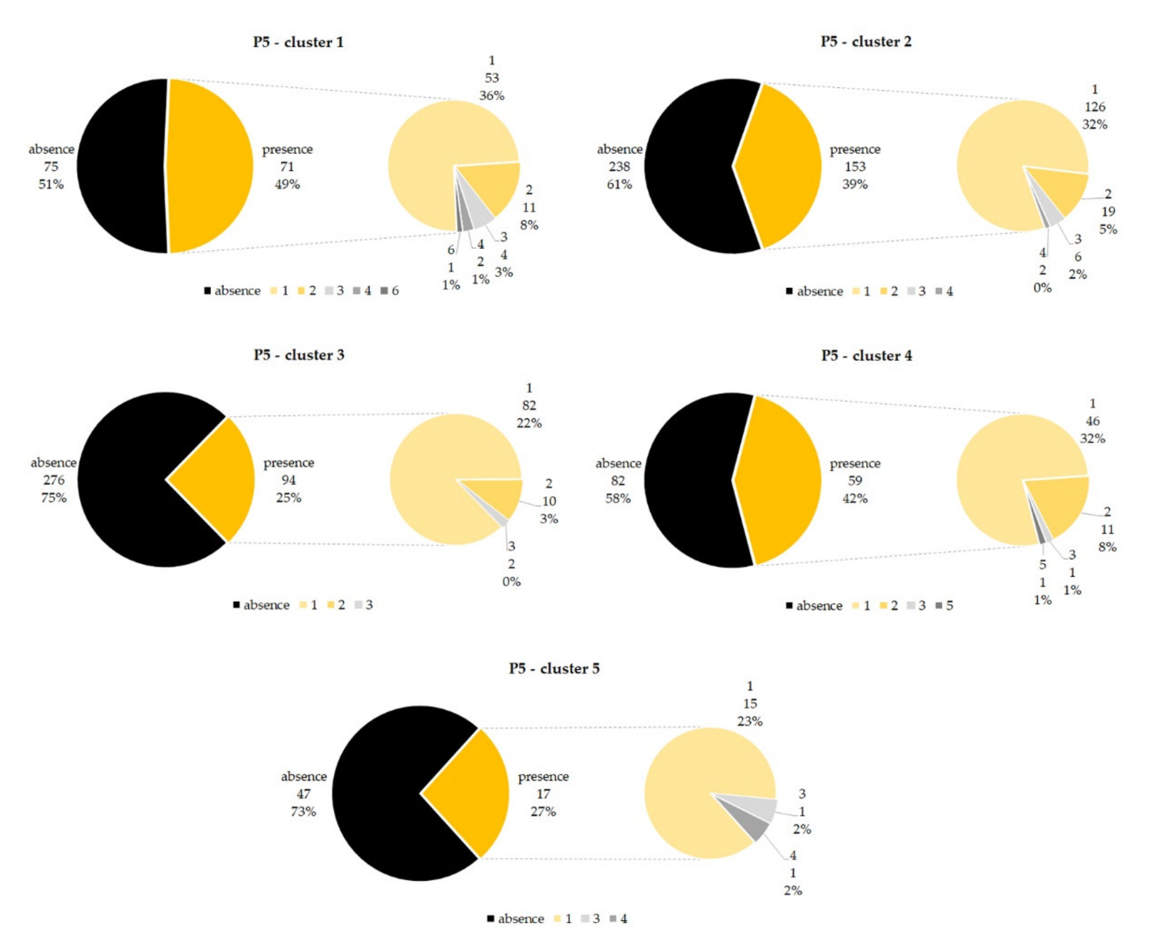
| P5 | Special building | Numbers of buildings with a special function, according to four categories: places of worship, public buildings, education, and cultural and tourism attractions |
| P6 | Construction technique | In terms of homogeneity of the construction technique, considering masonry as the prevalent type |
| P7 | Porches | Presence of porches along the perimeter of the OS (%) |
| P8 | Slope | Presence of sloped ground, in terms of maximum difference in height |
| P9 | Green | Presence of green space, in terms of percentage of green areas on the overall OS area |
| Database | Type of Database | Information |
|---|---|---|
| OpenStreetMaps (OSM) 1 | Open | Identification of squares; Function of building in OS perimeter; Identification of streets; Identification of green spaces |
| Edificato dei capoluoghi di provincia (Buildings of the capitals of the provinces) —Ministero Ambiente (MinAmb) 2 | Official | Height of buildings that define the OS perimeter; Height above sea level |
| Parameters | Source Database | OSM Research Query | Processing Tools | |
|---|---|---|---|---|
| P1 | Morphology | OSM | place = square; admin_level = 2; admin_level = 4; admin_level = 6; admin_level = 8; | Minimum oriented bounding box; Minimum circumscribed circumference; Inaccessibility pole; Intersection; Fix geometry; Join attributes by locations. |
| P2 | Height | OSM + MinAmb | place = square; layer building (MinAmb). | Buffer; Intersection; Fix geometry; Join attributes by locations. |
| P4 | Accesses | OSM | place = square; highway = pedestrian; highway = residential; highway = service; highway = living_street. | Merge; Intersection; Fix geometry; Join attributes by locations. |
| P5 | Special building | OSM | place = square; TOURISM: tourism = attraction; tourism = museum; PUBLIC: amenity = townhall; amenity = police; RELIGION: amenity = place_of_worship; building = church; building = temple; INSTRUCTION: amenity = university; amenity = school; amenity = college. | Merge; Intersection; Fix geometry; Join attributes by locations. |
| P8 | Slope | OSM + MinAmb | place = square; layer building (MinAmb). | Buffer; Merge; Intersection; Fix geometry; Join attributes by locations. |
| P9 | Green | OSM | place = square; leisure = park; leisure = garden; landuse = forest. | Merge; Intersection; Fix geometry; Join attributes by locations. |
| Parameters | Source Database | Data Set (Number of OSs) | Geographic Extension | |
|---|---|---|---|---|
| P1 | Morphology | OSM | 8889 | Italian territory |
| P2 | Critical height | OSM + MinAmb | 1392 | Capital of the province |
| P4 | Accesses | OSM | 1113 | Italian territory |
| P5 | Special building | OSM | 476 | Italian territory |
| P8 | Slope | OSM + MinAmb | 1392 | Capital of the province |
| P9 | Green | OSM | 8889 | Italian territory |
| Cluster | ||||||
|---|---|---|---|---|---|---|
| Parameter | 1 | 2 | 3 | 4 | 5 | Global Mean |
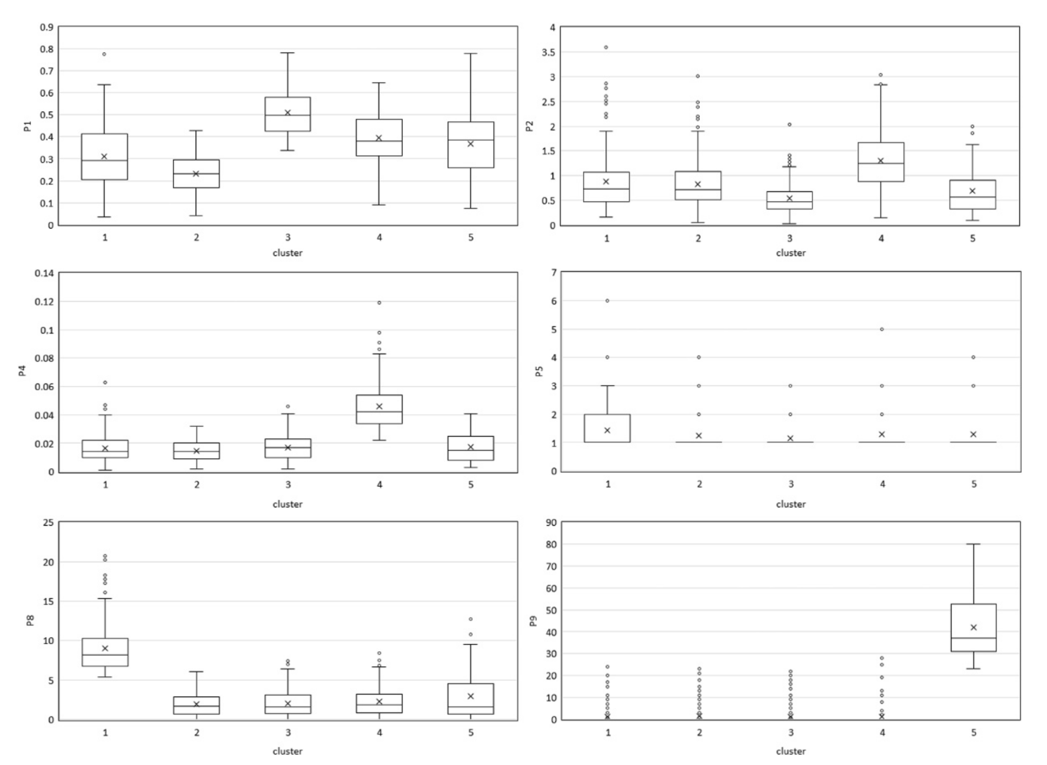
| P1 | 0.310 | 0.231 | 0.509 | 0.395 | 0.367 | 0.362 |
| P2 | 0.882 | 0.830 | 0.538 | 1.308 | 0.692 | 0.793 |
| P4 | 0.016 | 0.014 | 0.017 | 0.046 | 0.017 | 0.020 |
| P8 | 9.037 | 1.976 | 2.038 | 2.257 | 2.930 | 3.015 |
| P9 | 0.013 | 0.015 | 0.011 | 0.012 | 0.418 | 0.036 |
| Cases | 146 | 391 | 369 | 141 | 64 | 1111 |
| Type | Class 1 | Class 2 | Class 3 | |
|---|---|---|---|---|
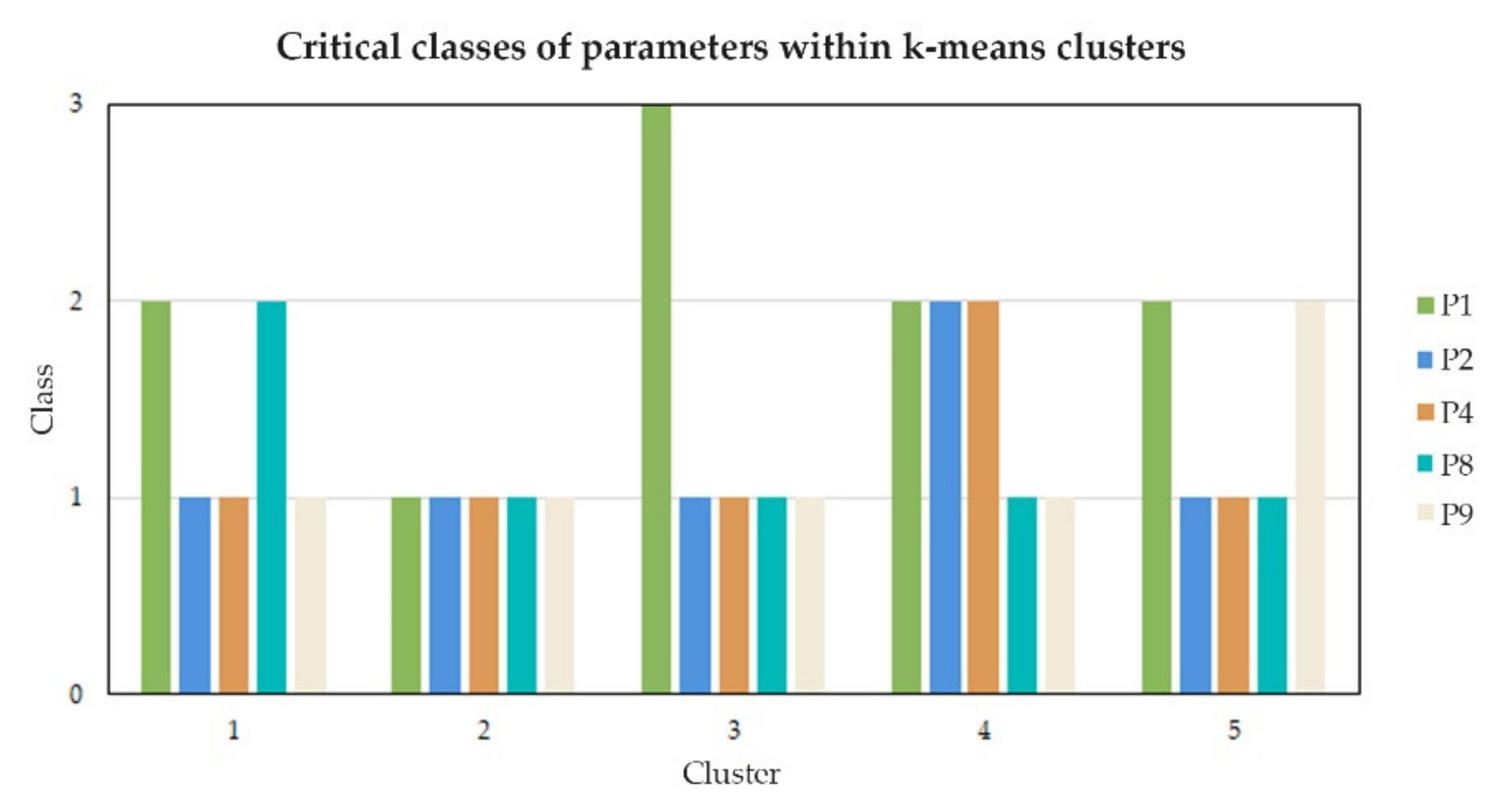
| P1 | Tripartite | P1 < 0.25 | 0.25 < P1 < 0.50 | P1 > 0.50 |
| low level of compactness and regularity | medium level of compactness and regularity | high level of compactness and regularity | ||
| P2 | Dichotomous | P2 < 1.00 | P2 ≥ 1.00 | - |
| no problems of overturning for the fronts | with overturning problems for the fronts | - | ||
| P4 | Dichotomous | P4 < 0.02 | P4 ≥ 0.02 | - |
| critical ratio between number of accesses/perimeter | no critical ratio between number of accesses/perimeter | - | ||
| P8 | Dichotomous | P8 < 3.00 | P8 ≥ 3.00 | - |
| flat or slightly sloping ground | sloping ground or changes in elevation | - | ||
| P9 | Dichotomous | P9 < 0.30 | P9 ≥ 0.30 | - |
| no green areas | presence of green areas | - |
| P1 | P2 | P4 | P5 | P8 | P9 | |
|---|---|---|---|---|---|---|
| 1 | 0.31 | 0.88 | 0.016 | 1.42 | 9.04 | 1.27 |
| (0.20–0.41) | (0.48–1.07) | (0.009–0.022) | (1–2) | (6.77–10.33) | (0–0) | |
| 2 | 0.23 | 0.83 | 0.014 | 1.24 | 1.98 | 1.5 |
| (0.17–0.30) | (0.51–1.08) | (0.009–0.020) | (1–1) | (0.70–2.90) | (0–0) | |
| 3 | 0.51 | 0.54 | 0.017 | 1.15 | 2.04 | 1.11 |
| (0.43–0.58) | (0.33–0.68) | (0.010–0.023) | (1–1) | (0.80–3.15) | (0–0) | |
| 4 | 0.4 | 1.31 | 0.046 | 1.29 | 2.26 | 1.22 |
| (0.31–0.48) | (0.89–1.67) | (0.034–0.054) | (1–1) | (0.85–3.20) | (0–0) | |
| 5 | 0.37 | 0.69 | 0.017 | 1.29 | 2.93 | 41.84 |
| (0.26–0.47) | (0.33–0.91) | (0.008–0.041) | (1–1) | (0.73–4.60) | (31–53) |
| P1 | P2 | P4 | P5 | |||||||
|---|---|---|---|---|---|---|---|---|---|---|
| BET | D1 (m) | D2 (m) | D2/D1 | Area Real (m2) | Area BB [m2] | A Real/ A BB | Hmean (m) | Hmax (m) | Accesses (Number) | SB (Number) |
| 1A | 101 | 41 | 0.41 (0.41–0.44) | 3441 (925–4940) | 4278 | 0.80 (0.57–0.81) | 15 | 26 | 3.8 | 1 |
| (53–127) | (22–56) | (1461–7299) | (12–19) | (19–32) | (2–5) | (1–2) | ||||
| 1B | 101 | 41 | 0.41 (0.41–0.44) | 3441 (925–4940) | 4278 | 0.80 (0.57–0.81) | 15 | - | 3.8 | 0 |
| (53–127) | (22–56) | (1461–7299) | (12–19) | (2–5) | ||||||
| 2A | 102 | 34 | 0.33 (0.27–0.42) | 2632 (1022–4038) | 3666 | 0.72 (0.55–0.75) | 15 | 23 | 3.6 | 1 |
| (62–127) | (21–42) | (1534–6287) | (10–19) | (16–28) | (2–5) | (1–1) | ||||
| 2B | 102 | 34 | 0.33 (0.27–0.42) | 2632 (1022–4038) | 3666 | 0.72 (0.55–0.75) | 15 | - | 3.6 | 0 |
| (62–127) | (21–42) | (1534–6287) | (10–19) | (2–5) | ||||||
| 3 | 85 | 49 | 0.56 (0.52–0.65) | 3430 (1167–4738) | 3430 | 1 | 15 | - | 3.5 | 0 |
| (49–105) | (30–60) | (1311–5441) | (0.79–0.95) | (11–19) | (2–5) | |||||
| 4A | 44 | 20 | 0.46 (0.42–0.58) | 720 (291–775) | 798 | 0.9 (0.72–0.90) | 16 | 22 | 4.6 | 1 |
| (28–50) | (13–24) | (366–1127) | (12–19) | (18–29) | (3–6) | (1–1) | ||||
| 4B | 44 (28–50) | 20 (13–24) | 0.46 (0.42–0.58) | 720 (291–775) | 798 (366–1127) | 0.9 (0.72–0.90) | 22 (18–29) | 22 (18–29) | 4.6 (3–6) | 1 (1–1) |
| 4C | 44 (28–50) | 20 (13–24 | 0.46 (0.42–0.58) | 720 (291–775) | 798 (366–1127) | 0.9 (0.72–0.90) | 22 (18–29) | - | 4.6 (3–6) | 0 |
| 5 | 104 (63–134) | 47 (26–57) | 0.45 (0.38–0.58) | 4185 (1115–5210) | 4743 (1739–7453) | 0.88 (0.64–0.90) | 16 (11–21) | - | 4 (2–5) | 0 |
| BET | OS | P1 | P2 | P4 | P5 | P8 | P9 |
|---|---|---|---|---|---|---|---|
| BET 1A | Piazza Grande, Arezzo | 0.48 | 0.48 | 0.012 | 3 | 11.80 | 0 |
| BET 1B | Piazza Vittorio Veneto, Torino | 0.31 | 0.22 | 0.022 | 0 | 5.70 | 0 |
| BET 2A | Piazza della Vittoria, Gorizia | 0.16 | 0.33 | 0.016 | 3 | 1.70 | 5 |
| BET 2B | Piazza degli Erri, Modena | 0.22 | 0.97 | 0.015 | 0 | 0.10 | 0 |
| BET 3 | Piazza della Repubblica, Firenze | 0.65 | 0.36 | 0.018 | 0 | 0.50 | 0 |
| BET 4A | Campo Sant‘Aponal, Venezia | 0.47 | 1.75 | 0.083 | 1 | 0.20 | 0 |
| BET 4B | Piazza della Pigna, Roma | 0.38 | 1.20 | 0.028 | 1 | 1.80 | 8 |
| BET 4C | Piazza Ramiro Ginocchio, La Spezia | 0.31 | 1.35 | 0.033 | 0 | 0.20 | 0 |
| BET 5 | Piazza Emilia, Milano | 0.41 | 0.52 | 0.005 | 0 | 0.50 | 32 |
| Risk | BET 1A | BET 1B | BET 2A | BET 2B | BET 3 | BET 4A | BET 4B | BET 4C | BET 5 |
|---|---|---|---|---|---|---|---|---|---|
| S | − | − | + | + | − | + | + | + | − |
| T | + | − | + | − | − | + | + | − | − |
| P | + | + | + | + | + | + | + | + | − |
| H | + | + | + | + | + | − | − | − | − |
| Characterizing risks | T + P + H | P + H | S + T + P + H | S + P + H | P + H | S + T + P | S + T + P | S + P | − |
Publisher’s Note: MDPI stays neutral with regard to jurisdictional claims in published maps and institutional affiliations. |
© 2021 by the authors. Licensee MDPI, Basel, Switzerland. This article is an open access article distributed under the terms and conditions of the Creative Commons Attribution (CC BY) license (https://creativecommons.org/licenses/by/4.0/).
Share and Cite
D’Amico, A.; Russo, M.; Angelosanti, M.; Bernardini, G.; Vicari, D.; Quagliarini, E.; Currà, E. Built Environment Typologies Prone to Risk: A Cluster Analysis of Open Spaces in Italian Cities. Sustainability 2021, 13, 9457. https://0-doi-org.brum.beds.ac.uk/10.3390/su13169457
D’Amico A, Russo M, Angelosanti M, Bernardini G, Vicari D, Quagliarini E, Currà E. Built Environment Typologies Prone to Risk: A Cluster Analysis of Open Spaces in Italian Cities. Sustainability. 2021; 13(16):9457. https://0-doi-org.brum.beds.ac.uk/10.3390/su13169457
Chicago/Turabian StyleD’Amico, Alessandro, Martina Russo, Marco Angelosanti, Gabriele Bernardini, Donatella Vicari, Enrico Quagliarini, and Edoardo Currà. 2021. "Built Environment Typologies Prone to Risk: A Cluster Analysis of Open Spaces in Italian Cities" Sustainability 13, no. 16: 9457. https://0-doi-org.brum.beds.ac.uk/10.3390/su13169457