
Impact of Shape Factor on Energy Demand, CO2 Emissions and Energy Cost of Residential Buildings in Cold Oceanic Climates: Case Study of South Chile


Abstract
:
1. Introduction
2. Materials and Methods
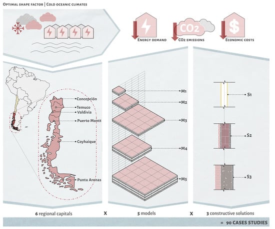
2.1. Shape Factor
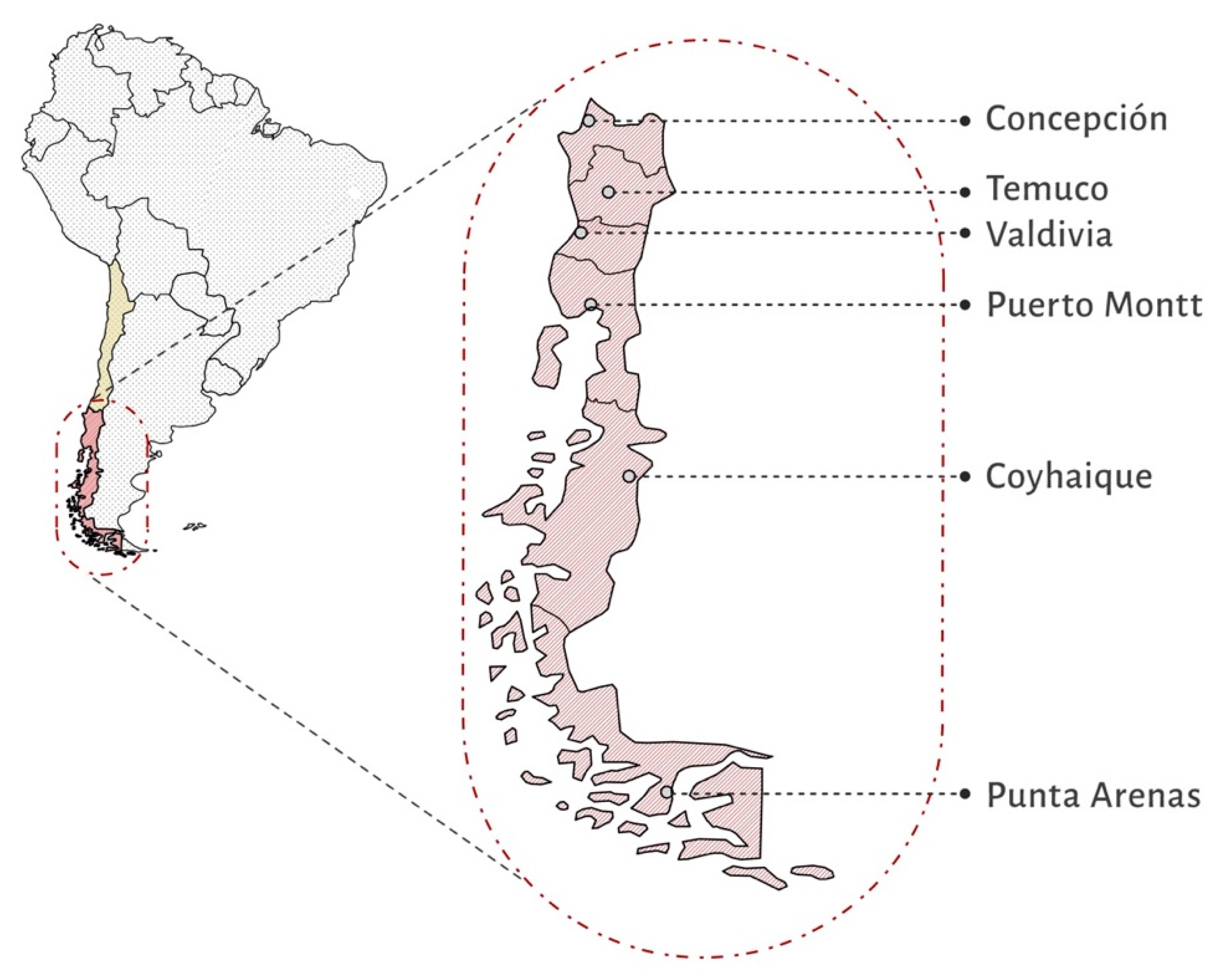
2.2. Climate Data and Climatic Zones
2.3. CO2 Emissions and Energy Costs of Fuels
2.4. Case Studies
2.4.1. Building Geometry
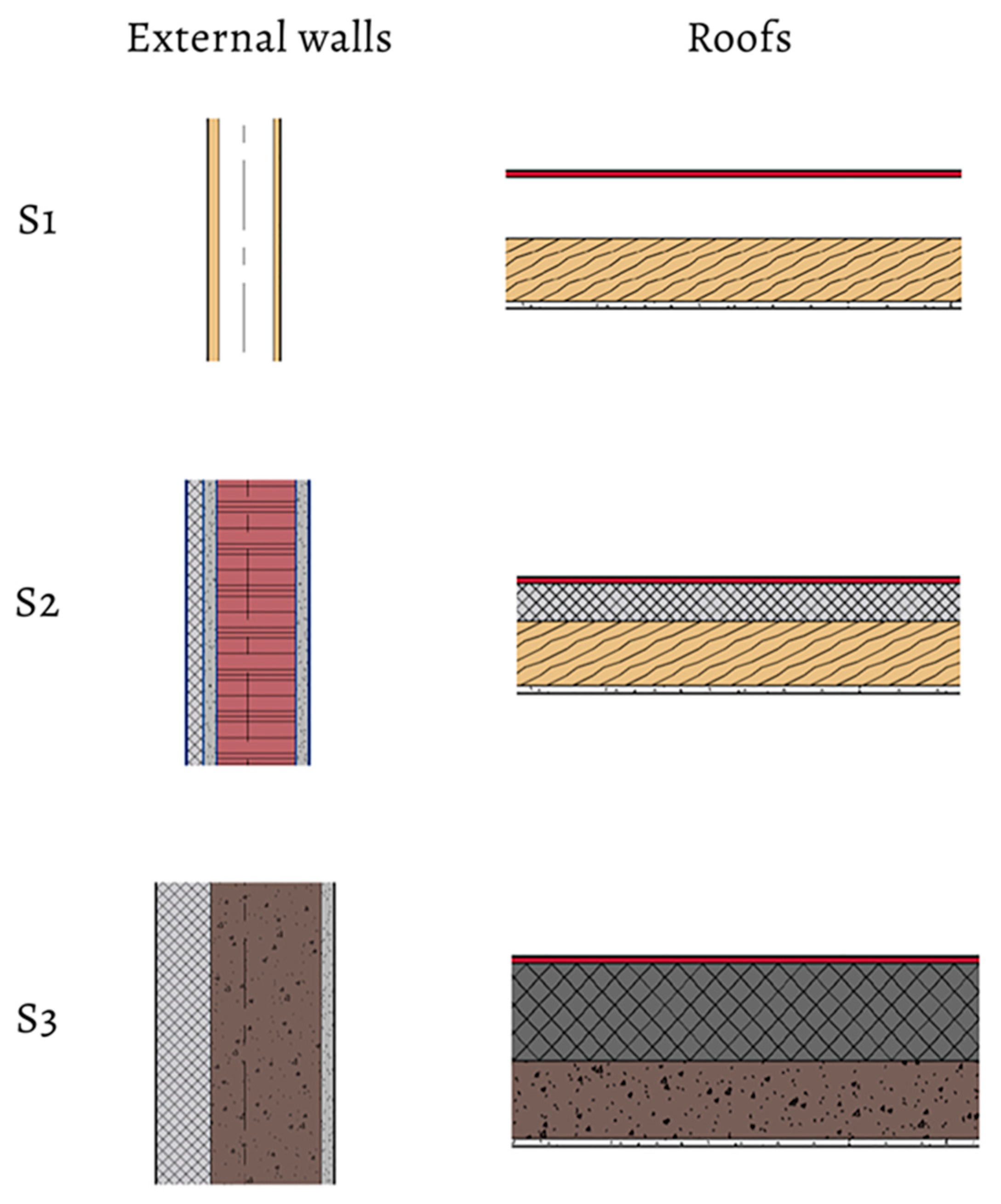
2.4.2. Architectural Designs for the Thermal Envelopes
3. Results
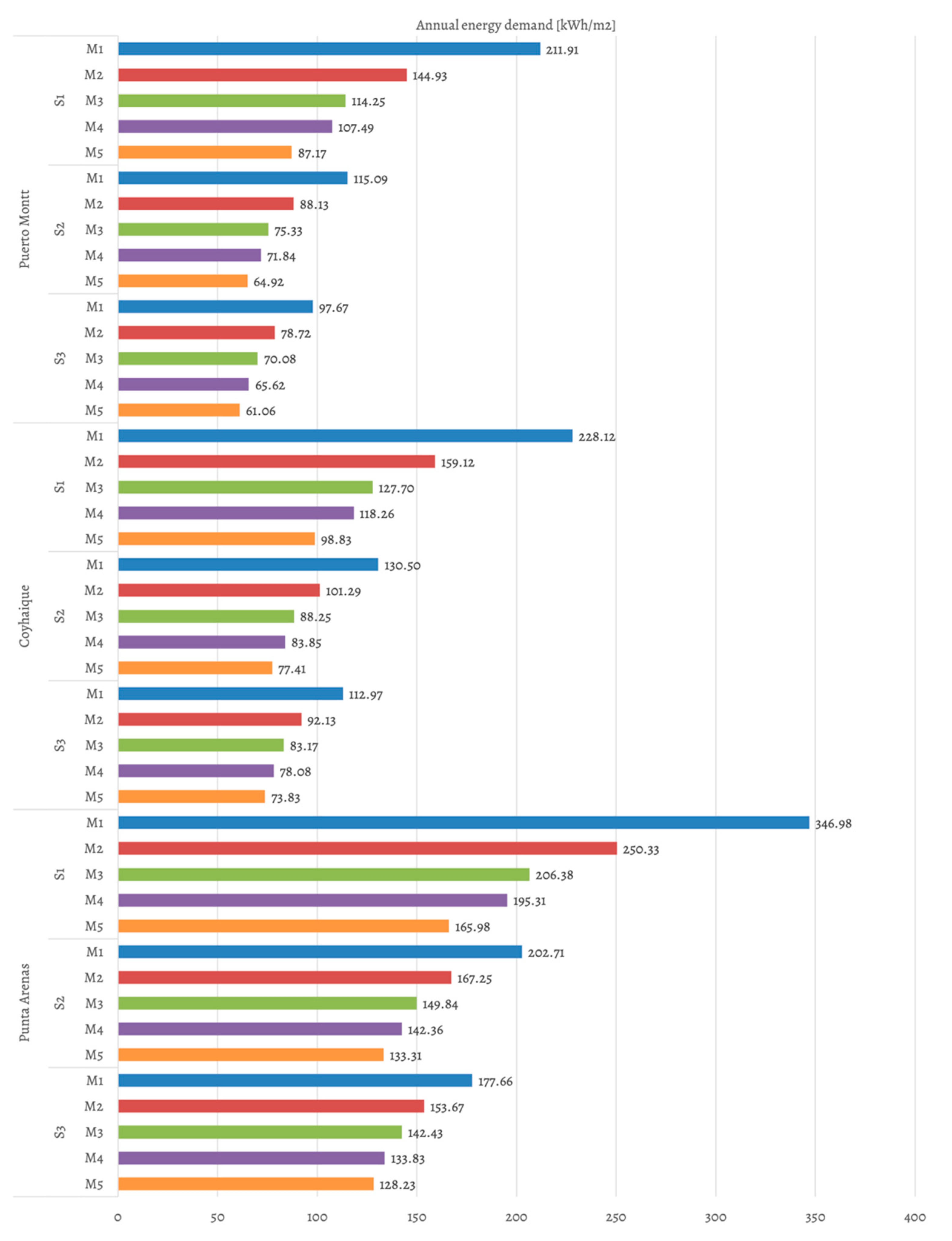
3.1. Energy Demand
3.2. CO2 Emissions
3.3. Energy Cost
4. Discussion
5. Conclusions
- The architectural designs with high thermal transmittance values may require from 129.44 to 227.67% of the energy demand of the same building after implementing a solution with a low U-value. Energy demand is widely affected by the weather where housing is located; maximum variations between 135.30 and 244.71% exist for the same SFv and architectural design, depending on the city where it is located.
- CO2 emissions depend directly on the climatic zone where the building is located and the fuel used. For all cities, using biomass in heating systems has the lowest emission and cost values, as opposed to what happens when using electricity for heating. Differences in CO2 emissions from 7.43 to 235.12% can be found between the different climatic zones for the same model. Similarly, the cost of the heating system is reduced by between 31.81 and 32.95% when switching from a fossil fuel, such as propane, to a renewable fuel, such as biomass in the form of pellets.
- Overall, the impact of SFv, on both energy demand and CO2 emissions, is greater when architectural designs with a high thermal transmittance value are implemented, reducing energy demand between 22.75% and 56.16%, depending on the area located. Based on the analysis, it is highly recommended to design buildings with a SFv below 0.767 for cold oceanic climates, such as in the southern zone of Chile. Among the values shown, energy demand and CO2 emissions tend to stabilise for all the climatic zones and construction solutions studied, with only 9.03% maximum differences in the energy requirement for heating and 10.37% in CO2 emissions.
Author Contributions
Funding
Institutional Review Board Statement
Informed Consent Statement
Conflicts of Interest
Appendix A

| Monthly Energy Demand [kWh/m2] | Annual Energy Demand [kWh/m2] | |||||||||||||||
|---|---|---|---|---|---|---|---|---|---|---|---|---|---|---|---|---|
| S | M | H/C | Jan. | Feb. | Mar. | Apr. | May | Jun. | Jul. | Aug. | Sep. | Oct. | Nov. | Dec. | H/C | Total |
| S1 | M1 | Heating | 4.10 | 4.18 | 6.49 | 11.73 | 16.63 | 19.54 | 21.38 | 18.22 | 15.97 | 11.14 | 7.94 | 5.13 | 142.45 | 147.46 |
| Cooling | 2.00 | 1.55 | 0.86 | 0.06 | 0.00 | 0.00 | 0.00 | 0.00 | 0.00 | 0.00 | 0.00 | 0.54 | 5.02 | |||
| M2 | Heating | 2.53 | 2.55 | 4.11 | 7.73 | 11.17 | 13.23 | 14.60 | 12.50 | 10.99 | 7.51 | 5.34 | 3.32 | 95.61 | 98.37 | |
| Cooling | 1.28 | 0.88 | 0.25 | 0.00 | 0.00 | 0.00 | 0.00 | 0.00 | 0.00 | 0.00 | 0.00 | 0.35 | 2.76 | |||
| M3 | Heating | 1.77 | 1.72 | 3.05 | 5.90 | 8.67 | 10.33 | 11.49 | 9.91 | 8.72 | 5.86 | 4.18 | 2.45 | 74.04 | 76.08 | |
| Cooling | 1.01 | 0.62 | 0.16 | 0.00 | 0.00 | 0.00 | 0.00 | 0.00 | 0.00 | 0.00 | 0.00 | 0.26 | 2.05 | |||
| M4 | Heating | 1.27 | 1.44 | 2.74 | 5.54 | 8.15 | 9.72 | 10.83 | 9.35 | 8.24 | 5.52 | 3.92 | 2.11 | 68.84 | 69.21 | |
| Cooling | 0.22 | 0.15 | 0.00 | 0.00 | 0.00 | 0.00 | 0.00 | 0.00 | 0.00 | 0.00 | 0.00 | 0.00 | 0.37 | |||
| M5 | Heating | 0.86 | 0.97 | 2.04 | 4.34 | 6.51 | 7.83 | 8.79 | 7.62 | 6.73 | 4.42 | 3.13 | 1.58 | 54.82 | 55.57 | |
| Cooling | 0.37 | 0.26 | 0.04 | 0.00 | 0.00 | 0.00 | 0.00 | 0.00 | 0.00 | 0.00 | 0.00 | 0.08 | 0.75 | |||
| S2 | M1 | Heating | 2.06 | 2.04 | 3.25 | 6.13 | 8.89 | 10.71 | 11.71 | 9.91 | 8.76 | 5.89 | 4.19 | 2.59 | 76.14 | 77.11 |
| Cooling | 0.29 | 0.51 | 0.08 | 0.00 | 0.00 | 0.00 | 0.00 | 0.00 | 0.00 | 0.00 | 0.00 | 0.08 | 0.96 | |||
| M2 | Heating | 1.35 | 1.26 | 2.23 | 4.41 | 6.60 | 7.99 | 8.91 | 7.63 | 6.76 | 4.42 | 3.11 | 1.80 | 56.46 | 56.85 | |
| Cooling | 0.20 | 0.20 | 0.00 | 0.00 | 0.00 | 0.00 | 0.00 | 0.00 | 0.00 | 0.00 | 0.00 | 0.00 | 0.39 | |||
| M3 | Heating | 0.88 | 0.92 | 1.74 | 3.62 | 5.54 | 6.75 | 7.60 | 6.57 | 5.83 | 3.74 | 2.63 | 1.39 | 47.21 | 47.54 | |
| Cooling | 0.15 | 0.18 | 0.00 | 0.00 | 0.00 | 0.00 | 0.00 | 0.00 | 0.00 | 0.00 | 0.00 | 0.00 | 0.33 | |||
| M4 | Heating | 0.61 | 0.71 | 1.53 | 3.47 | 5.31 | 6.49 | 7.29 | 6.25 | 5.55 | 3.53 | 2.48 | 1.19 | 44.40 | 44.66 | |
| Cooling | 0.15 | 0.11 | 0.00 | 0.00 | 0.00 | 0.00 | 0.00 | 0.00 | 0.00 | 0.00 | 0.00 | 0.00 | 0.26 | |||
| M5 | Heating | 0.49 | 0.53 | 1.20 | 3.02 | 4.75 | 5.83 | 6.59 | 5.69 | 5.06 | 3.18 | 2.20 | 0.93 | 39.48 | 39.78 | |
| Cooling | 0.18 | 0.13 | 0.00 | 0.00 | 0.00 | 0.00 | 0.00 | 0.00 | 0.00 | 0.00 | 0.00 | 0.00 | 0.30 | |||
| S3 | M1 | Heating | 1.64 | 1.62 | 2.63 | 5.08 | 7.47 | 9.06 | 9.94 | 8.40 | 7.45 | 4.94 | 3.50 | 2.12 | 63.85 | 64.77 |
| Cooling | 0.35 | 0.43 | 0.07 | 0.00 | 0.00 | 0.00 | 0.00 | 0.00 | 0.00 | 0.00 | 0.00 | 0.07 | 0.92 | |||
| M2 | Heating | 1.03 | 1.02 | 1.88 | 3.85 | 5.83 | 7.11 | 7.96 | 6.83 | 6.06 | 3.91 | 2.75 | 1.50 | 49.72 | 50.27 | |
| Cooling | 0.22 | 0.27 | 0.02 | 0.00 | 0.00 | 0.00 | 0.00 | 0.00 | 0.00 | 0.00 | 0.00 | 0.04 | 0.55 | |||
| M3 | Heating | 0.67 | 0.77 | 1.53 | 3.32 | 5.12 | 6.27 | 7.08 | 6.13 | 5.45 | 3.46 | 2.44 | 1.24 | 43.48 | 43.98 | |
| Cooling | 0.22 | 0.22 | 0.02 | 0.00 | 0.00 | 0.00 | 0.00 | 0.00 | 0.00 | 0.00 | 0.00 | 0.04 | 0.50 | |||
| M4 | Heating | 0.46 | 0.48 | 1.24 | 3.09 | 4.82 | 5.94 | 6.68 | 5.74 | 5.10 | 3.21 | 2.22 | 0.96 | 39.94 | 40.20 | |
| Cooling | 0.15 | 0.12 | 0.00 | 0.00 | 0.00 | 0.00 | 0.00 | 0.00 | 0.00 | 0.00 | 0.00 | 0.00 | 0.26 | |||
| M5 | Heating | 0.39 | 0.35 | 1.03 | 2.79 | 4.46 | 5.50 | 6.23 | 5.39 | 4.80 | 2.99 | 2.01 | 0.81 | 36.74 | 37.20 | |
| Cooling | 0.26 | 0.17 | 0.01 | 0.00 | 0.00 | 0.00 | 0.00 | 0.00 | 0.00 | 0.00 | 0.00 | 0.02 | 0.46 | |||
| Monthly Energy Demand [kWh/m2] | Annual Energy Demand [kWh/m2] | |||||||||||||||
|---|---|---|---|---|---|---|---|---|---|---|---|---|---|---|---|---|
| S | M | H/C | Jan. | Feb. | Mar. | Apr. | May | Jun. | Jul. | Aug. | Sep. | Oct. | Nov. | Dec. | H/C | Total |
| S1 | M1 | Heating | 6.26 | 6.04 | 9.74 | 15.70 | 20.42 | 24.09 | 26.89 | 22.80 | 19.25 | 14.23 | 10.94 | 7.62 | 183.97 | 195.74 |
| Cooling | 3.93 | 4.97 | 1.86 | 0.19 | 0.00 | 0.00 | 0.00 | 0.00 | 0.00 | 0.00 | 0.00 | 0.82 | 11.77 | |||
| M2 | Heating | 4.09 | 3.81 | 6.37 | 10.38 | 13.64 | 16.28 | 18.23 | 15.49 | 13.06 | 9.57 | 7.39 | 5.03 | 123.34 | 129.91 | |
| Cooling | 2.36 | 2.89 | 0.98 | 0.00 | 0.00 | 0.00 | 0.00 | 0.00 | 0.00 | 0.00 | 0.00 | 0.34 | 6.57 | |||
| M3 | Heating | 2.92 | 2.76 | 4.77 | 7.92 | 10.51 | 12.67 | 14.22 | 12.12 | 10.22 | 7.45 | 5.76 | 3.81 | 95.15 | 99.61 | |
| Cooling | 1.65 | 2.07 | 0.57 | 0.00 | 0.00 | 0.00 | 0.00 | 0.00 | 0.00 | 0.00 | 0.00 | 0.17 | 4.46 | |||
| M4 | Heating | 2.38 | 2.36 | 4.33 | 7.48 | 9.91 | 11.96 | 13.44 | 11.45 | 9.68 | 7.04 | 5.44 | 3.49 | 88.96 | 90.59 | |
| Cooling | 0.49 | 1.04 | 0.11 | 0.00 | 0.00 | 0.00 | 0.00 | 0.00 | 0.00 | 0.00 | 0.00 | 0.00 | 1.64 | |||
| M5 | Heating | 1.74 | 1.78 | 3.30 | 5.87 | 7.86 | 9.60 | 10.83 | 9.23 | 7.78 | 5.61 | 4.35 | 2.61 | 70.56 | 72.52 | |
| Cooling | 0.65 | 1.11 | 0.15 | 0.00 | 0.00 | 0.00 | 0.00 | 0.00 | 0.00 | 0.00 | 0.00 | 0.04 | 1.96 | |||
| S2 | M1 | Heating | 3.17 | 3.02 | 5.02 | 8.21 | 10.80 | 13.04 | 14.67 | 12.27 | 10.27 | 7.46 | 5.73 | 3.91 | 97.57 | 101.76 |
| Cooling | 1.35 | 2.21 | 0.63 | 0.00 | 0.00 | 0.00 | 0.00 | 0.00 | 0.00 | 0.00 | 0.00 | 0.00 | 4.19 | |||
| M2 | Heating | 2.15 | 2.06 | 3.56 | 5.94 | 7.93 | 9.74 | 10.97 | 9.28 | 7.78 | 5.59 | 4.32 | 2.81 | 72.14 | 73.93 | |
| Cooling | 0.62 | 0.98 | 0.19 | 0.00 | 0.00 | 0.00 | 0.00 | 0.00 | 0.00 | 0.00 | 0.00 | 0.00 | 1.79 | |||
| M3 | Heating | 1.63 | 1.56 | 2.83 | 4.88 | 6.61 | 8.20 | 9.27 | 7.87 | 6.60 | 4.71 | 3.65 | 2.29 | 60.10 | 61.54 | |
| Cooling | 0.53 | 0.76 | 0.14 | 0.00 | 0.00 | 0.00 | 0.00 | 0.00 | 0.00 | 0.00 | 0.00 | 0.00 | 1.43 | |||
| M4 | Heating | 1.26 | 1.35 | 2.57 | 4.72 | 6.39 | 7.93 | 8.97 | 7.58 | 6.34 | 4.50 | 3.48 | 2.05 | 57.13 | 58.20 | |
| Cooling | 0.23 | 0.83 | 0.00 | 0.00 | 0.00 | 0.00 | 0.00 | 0.00 | 0.00 | 0.00 | 0.00 | 0.00 | 1.07 | |||
| M5 | Heating | 1.04 | 1.13 | 2.17 | 4.13 | 5.68 | 7.11 | 8.07 | 6.83 | 5.71 | 4.03 | 3.13 | 1.77 | 50.81 | 52.18 | |
| Cooling | 0.44 | 0.80 | 0.12 | 0.00 | 0.00 | 0.00 | 0.00 | 0.00 | 0.00 | 0.00 | 0.00 | 0.00 | 1.37 | |||
| S3 | M1 | Heating | 2.61 | 2.49 | 4.14 | 6.82 | 9.03 | 11.01 | 12.40 | 10.37 | 8.65 | 6.24 | 4.79 | 3.23 | 81.79 | 85.80 |
| Cooling | 1.26 | 2.07 | 0.69 | 0.00 | 0.00 | 0.00 | 0.00 | 0.00 | 0.00 | 0.00 | 0.00 | 0.00 | 4.02 | |||
| M2 | Heating | 1.78 | 1.68 | 3.03 | 5.20 | 6.99 | 8.65 | 9.76 | 8.25 | 6.91 | 4.94 | 3.82 | 2.43 | 63.42 | 65.56 | |
| Cooling | 0.76 | 1.05 | 0.32 | 0.00 | 0.00 | 0.00 | 0.00 | 0.00 | 0.00 | 0.00 | 0.00 | 0.00 | 2.14 | |||
| M3 | Heating | 1.40 | 1.38 | 2.52 | 4.48 | 6.09 | 7.60 | 8.60 | 7.30 | 6.12 | 4.35 | 3.39 | 2.07 | 55.29 | 57.09 | |
| Cooling | 0.66 | 0.89 | 0.24 | 0.00 | 0.00 | 0.00 | 0.00 | 0.00 | 0.00 | 0.00 | 0.00 | 0.00 | 1.79 | |||
| M4 | Heating | 0.99 | 1.09 | 2.11 | 4.23 | 5.79 | 7.24 | 8.20 | 6.93 | 5.78 | 4.08 | 3.16 | 1.76 | 51.35 | 52.60 | |
| Cooling | 0.36 | 0.84 | 0.05 | 0.00 | 0.00 | 0.00 | 0.00 | 0.00 | 0.00 | 0.00 | 0.00 | 0.00 | 1.26 | |||
| M5 | Heating | 0.87 | 0.94 | 1.75 | 3.84 | 5.32 | 6.70 | 7.60 | 6.44 | 5.38 | 3.79 | 2.91 | 1.62 | 47.16 | 48.82 | |
| Cooling | 0.51 | 0.96 | 0.19 | 0.00 | 0.00 | 0.00 | 0.00 | 0.00 | 0.00 | 0.00 | 0.00 | 0.01 | 1.66 | |||
| Monthly Energy Demand [kWh/m2] | Annual Energy Demand [kWh/m2] | |||||||||||||||
|---|---|---|---|---|---|---|---|---|---|---|---|---|---|---|---|---|
| S | M | H/C | Jan. | Feb. | Mar. | Apr. | May | Jun. | Jul. | Aug. | Sep. | Oct. | Nov. | Dec. | H/C | Total |
| S1 | M1 | Heating | 6.08 | 5.93 | 9.55 | 15.29 | 21.17 | 24.95 | 27.41 | 23.60 | 19.14 | 14.45 | 11.12 | 7.76 | 186.45 | 198.16 |
| Cooling | 4.19 | 4.74 | 1.43 | 0.00 | 0.00 | 0.00 | 0.00 | 0.00 | 0.00 | 0.00 | 0.00 | 1.35 | 11.71 | |||
| M2 | Heating | 4.01 | 3.73 | 6.20 | 10.16 | 14.18 | 16.94 | 18.71 | 16.09 | 13.03 | 9.76 | 7.53 | 5.16 | 125.51 | 131.93 | |
| Cooling | 2.45 | 2.75 | 0.59 | 0.00 | 0.00 | 0.00 | 0.00 | 0.00 | 0.00 | 0.00 | 0.00 | 0.63 | 6.42 | |||
| M3 | Heating | 2.92 | 2.66 | 4.69 | 7.81 | 10.95 | 13.23 | 14.68 | 12.62 | 10.22 | 7.62 | 5.88 | 3.92 | 97.21 | 101.50 | |
| Cooling | 1.67 | 1.96 | 0.25 | 0.00 | 0.00 | 0.00 | 0.00 | 0.00 | 0.00 | 0.00 | 0.00 | 0.42 | 4.29 | |||
| M4 | Heating | 2.24 | 2.31 | 4.29 | 7.37 | 10.32 | 12.48 | 13.87 | 11.92 | 9.67 | 7.20 | 5.55 | 3.45 | 90.69 | 92.49 | |
| Cooling | 0.38 | 1.29 | 0.00 | 0.00 | 0.00 | 0.00 | 0.00 | 0.00 | 0.00 | 0.00 | 0.00 | 0.14 | 1.80 | |||
| M5 | Heating | 1.65 | 1.67 | 3.32 | 5.84 | 8.22 | 10.07 | 11.24 | 9.65 | 7.82 | 5.77 | 4.45 | 2.65 | 72.33 | 74.41 | |
| Cooling | 0.65 | 1.19 | 0.06 | 0.00 | 0.00 | 0.00 | 0.00 | 0.00 | 0.00 | 0.00 | 0.00 | 0.17 | 2.07 | |||
| S2 | M1 | Heating | 3.11 | 2.99 | 4.95 | 8.06 | 11.38 | 13.62 | 14.98 | 12.87 | 10.35 | 7.67 | 5.90 | 4.02 | 99.90 | 104.16 |
| Cooling | 1.30 | 2.31 | 0.28 | 0.00 | 0.00 | 0.00 | 0.00 | 0.00 | 0.00 | 0.00 | 0.00 | 0.36 | 4.26 | |||
| M2 | Heating | 2.18 | 1.98 | 3.51 | 5.89 | 8.36 | 10.25 | 11.38 | 9.75 | 7.84 | 5.77 | 4.46 | 2.94 | 74.32 | 76.46 | |
| Cooling | 0.64 | 1.27 | 0.05 | 0.00 | 0.00 | 0.00 | 0.00 | 0.00 | 0.00 | 0.00 | 0.00 | 0.18 | 2.15 | |||
| M3 | Heating | 1.60 | 1.56 | 2.81 | 4.89 | 6.97 | 8.66 | 9.67 | 8.28 | 6.68 | 4.88 | 3.78 | 2.32 | 62.11 | 63.89 | |
| Cooling | 0.57 | 1.00 | 0.04 | 0.00 | 0.00 | 0.00 | 0.00 | 0.00 | 0.00 | 0.00 | 0.00 | 0.17 | 1.78 | |||
| M4 | Heating | 1.19 | 1.29 | 2.62 | 4.72 | 6.75 | 8.37 | 9.34 | 7.99 | 6.41 | 4.67 | 3.60 | 2.05 | 58.99 | 60.14 | |
| Cooling | 0.18 | 0.97 | 0.00 | 0.00 | 0.00 | 0.00 | 0.00 | 0.00 | 0.00 | 0.00 | 0.00 | 0.00 | 1.15 | |||
| M5 | Heating | 1.00 | 1.03 | 2.22 | 4.20 | 6.01 | 7.53 | 8.43 | 7.21 | 5.80 | 4.20 | 3.21 | 1.81 | 52.65 | 54.25 | |
| Cooling | 0.48 | 0.96 | 0.01 | 0.00 | 0.00 | 0.00 | 0.00 | 0.00 | 0.00 | 0.00 | 0.00 | 0.15 | 1.61 | |||
| S3 | M1 | Heating | 2.57 | 2.44 | 4.07 | 6.72 | 9.56 | 11.55 | 12.71 | 10.91 | 8.75 | 6.44 | 4.96 | 3.34 | 84.02 | 88.02 |
| Cooling | 1.32 | 2.03 | 0.30 | 0.00 | 0.00 | 0.00 | 0.00 | 0.00 | 0.00 | 0.00 | 0.00 | 0.34 | 3.99 | |||
| M2 | Heating | 1.75 | 1.69 | 3.01 | 5.18 | 7.39 | 9.12 | 10.15 | 8.70 | 6.99 | 5.12 | 3.96 | 2.49 | 65.53 | 67.93 | |
| Cooling | 0.83 | 1.20 | 0.13 | 0.00 | 0.00 | 0.00 | 0.00 | 0.00 | 0.00 | 0.00 | 0.00 | 0.23 | 2.39 | |||
| M3 | Heating | 1.32 | 1.32 | 2.54 | 4.51 | 6.44 | 8.04 | 8.99 | 7.70 | 6.21 | 4.53 | 3.51 | 2.02 | 57.11 | 59.12 | |
| Cooling | 0.75 | 0.97 | 0.09 | 0.00 | 0.00 | 0.00 | 0.00 | 0.00 | 0.00 | 0.00 | 0.00 | 0.21 | 2.01 | |||
| M4 | Heating | 0.92 | 0.98 | 2.25 | 4.27 | 6.13 | 7.66 | 8.56 | 7.31 | 5.86 | 4.25 | 3.25 | 1.82 | 53.27 | 54.69 | |
| Cooling | 0.37 | 0.96 | 0.00 | 0.00 | 0.00 | 0.00 | 0.00 | 0.00 | 0.00 | 0.00 | 0.00 | 0.09 | 1.42 | |||
| M5 | Heating | 0.84 | 0.85 | 1.99 | 3.93 | 5.64 | 7.10 | 7.97 | 6.80 | 5.47 | 3.95 | 3.01 | 1.69 | 49.22 | 51.16 | |
| Cooling | 0.68 | 0.98 | 0.07 | 0.00 | 0.00 | 0.00 | 0.00 | 0.00 | 0.00 | 0.00 | 0.00 | 0.20 | 1.94 | |||
| Monthly Energy Demand [kWh/m2] | Annual Energy Demand [kWh/m2] | |||||||||||||||
|---|---|---|---|---|---|---|---|---|---|---|---|---|---|---|---|---|
| S | M | H/C | Jan. | Feb. | Mar. | Apr. | May | Jun. | Jul. | Aug. | Sep. | Oct. | Nov. | Dec. | H/C | Total |
| S1 | M1 | Heating | 7.11 | 7.06 | 11.37 | 16.92 | 22.88 | 27.66 | 29.23 | 26.72 | 22.28 | 17.13 | 13.66 | 9.45 | 211.46 | 211.91 |
| Cooling | 0.06 | 0.39 | 0.00 | 0.00 | 0.00 | 0.00 | 0.00 | 0.00 | 0.00 | 0.00 | 0.00 | 0.00 | 0.45 | |||
| M2 | Heating | 4.71 | 4.66 | 7.52 | 11.40 | 15.62 | 19.05 | 20.19 | 18.57 | 15.44 | 11.83 | 9.38 | 6.35 | 144.71 | 144.93 | |
| Cooling | 0.00 | 0.22 | 0.00 | 0.00 | 0.00 | 0.00 | 0.00 | 0.00 | 0.00 | 0.00 | 0.00 | 0.00 | 0.22 | |||
| M3 | Heating | 3.63 | 3.56 | 5.77 | 8.88 | 12.28 | 15.06 | 16.01 | 14.82 | 12.30 | 9.43 | 7.43 | 4.93 | 114.09 | 114.25 | |
| Cooling | 0.00 | 0.17 | 0.00 | 0.00 | 0.00 | 0.00 | 0.00 | 0.00 | 0.00 | 0.00 | 0.00 | 0.00 | 0.17 | |||
| M4 | Heating | 3.36 | 3.18 | 5.42 | 8.38 | 11.58 | 14.19 | 15.11 | 14.01 | 11.65 | 8.93 | 7.03 | 4.64 | 107.49 | 107.49 | |
| Cooling | 0.00 | 0.00 | 0.00 | 0.00 | 0.00 | 0.00 | 0.00 | 0.00 | 0.00 | 0.00 | 0.00 | 0.00 | 0.00 | |||
| M5 | Heating | 2.58 | 2.42 | 4.24 | 6.72 | 9.38 | 11.60 | 12.37 | 11.55 | 9.56 | 7.31 | 5.72 | 3.69 | 87.13 | 87.17 | |
| Cooling | 0.00 | 0.05 | 0.00 | 0.00 | 0.00 | 0.00 | 0.00 | 0.00 | 0.00 | 0.00 | 0.00 | 0.00 | 0.05 | |||
| S2 | M1 | Heating | 3.65 | 3.63 | 5.88 | 9.06 | 12.45 | 15.49 | 16.30 | 14.95 | 12.26 | 9.23 | 7.30 | 4.90 | 115.09 | 115.09 |
| Cooling | 0.00 | 0.00 | 0.00 | 0.00 | 0.00 | 0.00 | 0.00 | 0.00 | 0.00 | 0.00 | 0.00 | 0.00 | 0.00 | |||
| M2 | Heating | 2.65 | 2.64 | 4.29 | 6.77 | 9.47 | 11.85 | 12.56 | 11.66 | 9.61 | 7.27 | 5.69 | 3.68 | 88.13 | 88.13 | |
| Cooling | 0.00 | 0.00 | 0.00 | 0.00 | 0.00 | 0.00 | 0.00 | 0.00 | 0.00 | 0.00 | 0.00 | 0.00 | 0.00 | |||
| M3 | Heating | 2.19 | 2.14 | 3.55 | 5.71 | 8.07 | 10.13 | 10.79 | 10.11 | 8.31 | 6.31 | 4.90 | 3.10 | 75.33 | 75.33 | |
| Cooling | 0.00 | 0.00 | 0.00 | 0.00 | 0.00 | 0.00 | 0.00 | 0.00 | 0.00 | 0.00 | 0.00 | 0.00 | 0.00 | |||
| M4 | Heating | 1.98 | 1.90 | 3.38 | 5.47 | 7.74 | 9.78 | 10.40 | 9.69 | 7.95 | 5.97 | 4.64 | 2.93 | 71.84 | 71.84 | |
| Cooling | 0.00 | 0.00 | 0.00 | 0.00 | 0.00 | 0.00 | 0.00 | 0.00 | 0.00 | 0.00 | 0.00 | 0.00 | 0.00 | |||
| M5 | Heating | 1.70 | 1.61 | 2.94 | 4.92 | 7.00 | 8.87 | 9.46 | 8.87 | 7.26 | 5.48 | 4.24 | 2.58 | 64.92 | 64.92 | |
| Cooling | 0.00 | 0.00 | 0.00 | 0.00 | 0.00 | 0.00 | 0.00 | 0.00 | 0.00 | 0.00 | 0.00 | 0.00 | 0.00 | |||
| S3 | M1 | Heating | 3.01 | 3.01 | 4.88 | 7.62 | 10.55 | 13.26 | 13.94 | 12.82 | 10.47 | 7.84 | 6.18 | 4.08 | 97.67 | 97.67 |
| Cooling | 0.00 | 0.00 | 0.00 | 0.00 | 0.00 | 0.00 | 0.00 | 0.00 | 0.00 | 0.00 | 0.00 | 0.00 | 0.00 | |||
| M2 | Heating | 2.31 | 2.29 | 3.75 | 5.99 | 8.45 | 10.64 | 11.29 | 10.51 | 8.64 | 6.52 | 5.08 | 3.24 | 78.72 | 78.72 | |
| Cooling | 0.00 | 0.00 | 0.00 | 0.00 | 0.00 | 0.00 | 0.00 | 0.00 | 0.00 | 0.00 | 0.00 | 0.00 | 0.00 | |||
| M3 | Heating | 1.98 | 1.90 | 3.24 | 5.29 | 7.51 | 9.46 | 10.08 | 9.48 | 7.78 | 5.90 | 4.58 | 2.87 | 70.08 | 70.08 | |
| Cooling | 0.00 | 0.00 | 0.00 | 0.00 | 0.00 | 0.00 | 0.00 | 0.00 | 0.00 | 0.00 | 0.00 | 0.00 | 0.00 | |||
| M4 | Heating | 1.71 | 1.61 | 2.97 | 4.98 | 7.10 | 9.01 | 9.59 | 8.96 | 7.33 | 5.50 | 4.26 | 2.59 | 65.62 | 65.62 | |
| Cooling | 0.00 | 0.00 | 0.00 | 0.00 | 0.00 | 0.00 | 0.00 | 0.00 | 0.00 | 0.00 | 0.00 | 0.00 | 0.00 | |||
| M5 | Heating | 1.47 | 1.47 | 2.66 | 4.63 | 6.62 | 8.40 | 8.97 | 8.43 | 6.90 | 5.20 | 4.01 | 2.30 | 61.06 | 61.06 | |
| Cooling | 0.00 | 0.00 | 0.00 | 0.00 | 0.00 | 0.00 | 0.00 | 0.00 | 0.00 | 0.00 | 0.00 | 0.00 | 0.00 | |||
| Monthly Energy Demand [kWh/m2] | Annual Energy Demand [kWh/m2] | |||||||||||||||
|---|---|---|---|---|---|---|---|---|---|---|---|---|---|---|---|---|
| S | M | H/C | Jan. | Feb. | Mar. | Apr. | May | Jun. | Jul. | Aug. | Sep. | Oct. | Nov. | Dec. | H/C | Total |
| S1 | M1 | Heating | 3.57 | 4.50 | 7.70 | 15.05 | 27.17 | 33.15 | 37.66 | 29.82 | 22.12 | 14.53 | 10.14 | 5.41 | 210.82 | 228.12 |
| Cooling | 6.51 | 6.79 | 0.96 | 0.00 | 0.00 | 0.00 | 0.00 | 0.00 | 0.00 | 0.00 | 0.07 | 2.98 | 17.30 | |||
| M2 | Heating | 2.22 | 2.98 | 5.23 | 10.38 | 18.99 | 23.41 | 26.63 | 21.23 | 15.85 | 10.30 | 7.18 | 3.68 | 148.08 | 159.12 | |
| Cooling | 4.26 | 4.29 | 0.61 | 0.00 | 0.00 | 0.00 | 0.00 | 0.00 | 0.00 | 0.00 | 0.00 | 1.88 | 11.04 | |||
| M3 | Heating | 1.64 | 2.26 | 4.11 | 8.27 | 15.23 | 18.90 | 21.53 | 17.30 | 13.03 | 8.40 | 5.88 | 2.87 | 119.40 | 127.70 | |
| Cooling | 3.19 | 3.24 | 0.47 | 0.00 | 0.00 | 0.00 | 0.00 | 0.00 | 0.00 | 0.00 | 0.00 | 1.40 | 8.29 | |||
| M4 | Heating | 1.41 | 1.99 | 3.66 | 7.77 | 14.34 | 17.81 | 20.33 | 16.35 | 12.33 | 7.93 | 5.49 | 2.54 | 111.95 | 118.26 | |
| Cooling | 2.42 | 2.64 | 0.26 | 0.00 | 0.00 | 0.00 | 0.00 | 0.00 | 0.00 | 0.00 | 0.00 | 0.98 | 6.31 | |||
| M5 | Heating | 1.12 | 1.60 | 2.92 | 6.37 | 11.88 | 14.87 | 17.01 | 13.72 | 10.42 | 6.65 | 4.60 | 2.02 | 93.18 | 98.83 | |
| Cooling | 2.12 | 2.27 | 0.36 | 0.00 | 0.00 | 0.00 | 0.00 | 0.00 | 0.00 | 0.00 | 0.00 | 0.90 | 5.65 | |||
| S2 | M1 | Heating | 1.78 | 2.45 | 4.20 | 8.44 | 15.64 | 19.26 | 21.93 | 17.15 | 12.72 | 8.21 | 5.75 | 2.92 | 120.45 | 130.50 |
| Cooling | 3.93 | 4.12 | 0.43 | 0.00 | 0.00 | 0.00 | 0.00 | 0.00 | 0.00 | 0.00 | 0.00 | 1.57 | 10.05 | |||
| M2 | Heating | 1.28 | 1.78 | 3.17 | 6.48 | 12.16 | 15.21 | 17.35 | 13.87 | 10.44 | 6.64 | 4.67 | 2.19 | 95.22 | 101.29 | |
| Cooling | 2.37 | 2.46 | 0.32 | 0.00 | 0.00 | 0.00 | 0.00 | 0.00 | 0.00 | 0.00 | 0.00 | 0.91 | 6.06 | |||
| M3 | Heating | 1.03 | 1.52 | 2.67 | 5.60 | 10.55 | 13.28 | 15.19 | 12.25 | 9.33 | 5.91 | 4.15 | 1.86 | 83.35 | 88.25 | |
| Cooling | 1.86 | 2.02 | 0.27 | 0.00 | 0.00 | 0.00 | 0.00 | 0.00 | 0.00 | 0.00 | 0.00 | 0.74 | 4.90 | |||
| M4 | Heating | 0.88 | 1.30 | 2.32 | 5.31 | 10.14 | 12.78 | 14.62 | 11.70 | 8.83 | 5.55 | 3.83 | 1.59 | 78.85 | 83.85 | |
| Cooling | 1.82 | 2.07 | 0.32 | 0.00 | 0.00 | 0.00 | 0.00 | 0.00 | 0.00 | 0.00 | 0.00 | 0.79 | 5.00 | |||
| M5 | Heating | 0.78 | 1.20 | 2.09 | 4.83 | 9.29 | 11.75 | 13.48 | 10.84 | 8.25 | 5.18 | 3.57 | 1.43 | 72.68 | 77.41 | |
| Cooling | 1.85 | 1.84 | 0.33 | 0.00 | 0.00 | 0.00 | 0.00 | 0.00 | 0.00 | 0.00 | 0.00 | 0.70 | 4.73 | |||
| S3 | M1 | Heating | 1.48 | 2.06 | 3.56 | 7.22 | 13.50 | 16.74 | 19.07 | 14.92 | 11.07 | 7.09 | 4.97 | 2.42 | 104.10 | 112.97 |
| Cooling | 3.48 | 3.56 | 0.43 | 0.00 | 0.00 | 0.00 | 0.00 | 0.00 | 0.00 | 0.00 | 0.00 | 1.40 | 8.87 | |||
| M2 | Heating | 1.08 | 1.60 | 2.80 | 5.83 | 11.02 | 13.84 | 15.80 | 12.65 | 9.55 | 6.05 | 4.25 | 1.96 | 86.43 | 92.13 | |
| Cooling | 2.26 | 2.28 | 0.31 | 0.00 | 0.00 | 0.00 | 0.00 | 0.00 | 0.00 | 0.00 | 0.00 | 0.85 | 5.70 | |||
| M3 | Heating | 0.93 | 1.35 | 2.40 | 5.25 | 9.92 | 12.52 | 14.33 | 11.57 | 8.85 | 5.60 | 3.93 | 1.66 | 78.32 | 83.17 | |
| Cooling | 1.86 | 1.96 | 0.30 | 0.00 | 0.00 | 0.00 | 0.00 | 0.00 | 0.00 | 0.00 | 0.00 | 0.73 | 4.85 | |||
| M4 | Heating | 0.77 | 1.18 | 2.08 | 4.88 | 9.41 | 11.91 | 13.64 | 10.92 | 8.27 | 5.18 | 3.53 | 1.39 | 73.18 | 78.08 | |
| Cooling | 1.87 | 1.94 | 0.35 | 0.00 | 0.00 | 0.00 | 0.00 | 0.00 | 0.00 | 0.00 | 0.00 | 0.73 | 4.90 | |||
| M5 | Heating | 0.71 | 1.12 | 1.89 | 4.57 | 8.85 | 11.23 | 12.89 | 10.38 | 7.92 | 4.95 | 3.36 | 1.30 | 69.18 | 73.83 | |
| Cooling | 1.82 | 1.81 | 0.33 | 0.00 | 0.00 | 0.00 | 0.00 | 0.00 | 0.00 | 0.00 | 0.00 | 0.68 | 4.65 | |||
| Monthly Energy Demand [kWh/m2] | Annual Energy Demand [kWh/m2] | |||||||||||||||
|---|---|---|---|---|---|---|---|---|---|---|---|---|---|---|---|---|
| S | M | H/C | Jan. | Feb. | Mar. | Apr. | May | Jun. | Jul. | Aug. | Sep. | Oct. | Nov. | Dec. | H/C | Total |
| S1 | M1 | Heating | 14.15 | 13.53 | 21.10 | 29.19 | 39.38 | 46.34 | 48.17 | 42.56 | 32.21 | 26.08 | 20.01 | 14.25 | 346.98 | 346.98 |
| Cooling | 0.00 | 0.00 | 0.00 | 0.00 | 0.00 | 0.00 | 0.00 | 0.00 | 0.00 | 0.00 | 0.00 | 0.00 | 0.00 | |||
| M2 | Heating | 10.39 | 9.72 | 15.10 | 20.85 | 27.99 | 32.80 | 34.20 | 30.59 | 23.59 | 19.40 | 15.13 | 10.57 | 250.33 | 250.33 | |
| Cooling | 0.00 | 0.00 | 0.00 | 0.00 | 0.00 | 0.00 | 0.00 | 0.00 | 0.00 | 0.00 | 0.00 | 0.00 | 0.00 | |||
| M3 | Heating | 8.75 | 8.03 | 12.44 | 17.02 | 22.71 | 26.50 | 27.70 | 25.07 | 19.66 | 16.43 | 13.02 | 9.03 | 206.38 | 206.38 | |
| Cooling | 0.00 | 0.00 | 0.00 | 0.00 | 0.00 | 0.00 | 0.00 | 0.00 | 0.00 | 0.00 | 0.00 | 0.00 | 0.00 | |||
| M4 | Heating | 8.28 | 7.59 | 11.77 | 16.06 | 21.42 | 25.00 | 26.15 | 23.69 | 18.64 | 15.66 | 12.44 | 8.62 | 195.31 | 195.31 | |
| Cooling | 0.00 | 0.00 | 0.00 | 0.00 | 0.00 | 0.00 | 0.00 | 0.00 | 0.00 | 0.00 | 0.00 | 0.00 | 0.00 | |||
| M5 | Heating | 7.13 | 6.44 | 9.97 | 13.54 | 17.97 | 20.95 | 21.95 | 20.04 | 15.93 | 13.59 | 10.93 | 7.54 | 165.98 | 165.98 | |
| Cooling | 0.00 | 0.00 | 0.00 | 0.00 | 0.00 | 0.00 | 0.00 | 0.00 | 0.00 | 0.00 | 0.00 | 0.00 | 0.00 | |||
| S2 | M1 | Heating | 8.06 | 7.66 | 12.11 | 17.06 | 23.13 | 27.49 | 28.50 | 25.15 | 18.74 | 15.19 | 11.55 | 8.07 | 202.71 | 202.71 |
| Cooling | 0.00 | 0.00 | 0.00 | 0.00 | 0.00 | 0.00 | 0.00 | 0.00 | 0.00 | 0.00 | 0.00 | 0.00 | 0.00 | |||
| M2 | Heating | 6.99 | 6.40 | 9.96 | 13.76 | 18.39 | 21.55 | 22.51 | 20.41 | 15.97 | 13.43 | 10.64 | 7.23 | 167.25 | 167.25 | |
| Cooling | 0.00 | 0.00 | 0.00 | 0.00 | 0.00 | 0.00 | 0.00 | 0.00 | 0.00 | 0.00 | 0.00 | 0.00 | 0.00 | |||
| M3 | Heating | 6.45 | 5.78 | 8.96 | 12.18 | 16.13 | 18.81 | 19.70 | 18.09 | 14.42 | 12.42 | 10.03 | 6.87 | 149.84 | 149.84 | |
| Cooling | 0.00 | 0.00 | 0.00 | 0.00 | 0.00 | 0.00 | 0.00 | 0.00 | 0.00 | 0.00 | 0.00 | 0.00 | 0.00 | |||
| M4 | Heating | 5.96 | 5.39 | 8.42 | 11.62 | 15.53 | 18.22 | 19.06 | 17.37 | 13.68 | 11.60 | 9.26 | 6.25 | 142.36 | 142.36 | |
| Cooling | 0.00 | 0.00 | 0.00 | 0.00 | 0.00 | 0.00 | 0.00 | 0.00 | 0.00 | 0.00 | 0.00 | 0.00 | 0.00 | |||
| M5 | Heating | 5.70 | 5.08 | 7.91 | 10.79 | 14.33 | 16.76 | 17.56 | 16.14 | 12.87 | 11.10 | 8.98 | 6.10 | 133.31 | 133.31 | |
| Cooling | 0.00 | 0.00 | 0.00 | 0.00 | 0.00 | 0.00 | 0.00 | 0.00 | 0.00 | 0.00 | 0.00 | 0.00 | 0.00 | |||
| S3 | M1 | Heating | 7.06 | 6.67 | 10.53 | 14.89 | 20.18 | 23.98 | 24.88 | 22.07 | 16.53 | 13.46 | 10.31 | 7.09 | 177.66 | 177.66 |
| Cooling | 0.00 | 0.00 | 0.00 | 0.00 | 0.00 | 0.00 | 0.00 | 0.00 | 0.00 | 0.00 | 0.00 | 0.00 | 0.00 | |||
| M2 | Heating | 6.46 | 5.87 | 9.13 | 12.58 | 16.79 | 19.67 | 20.56 | 18.72 | 14.73 | 12.48 | 9.95 | 6.74 | 153.67 | 153.67 | |
| Cooling | 0.00 | 0.00 | 0.00 | 0.00 | 0.00 | 0.00 | 0.00 | 0.00 | 0.00 | 0.00 | 0.00 | 0.00 | 0.00 | |||
| M3 | Heating | 6.18 | 5.50 | 8.51 | 11.53 | 15.24 | 17.77 | 18.62 | 17.15 | 13.73 | 11.91 | 9.68 | 6.63 | 142.43 | 142.43 | |
| Cooling | 0.00 | 0.00 | 0.00 | 0.00 | 0.00 | 0.00 | 0.00 | 0.00 | 0.00 | 0.00 | 0.00 | 0.00 | 0.00 | |||
| M4 | Heating | 5.63 | 5.06 | 7.91 | 10.88 | 14.51 | 17.01 | 17.81 | 16.30 | 12.89 | 11.02 | 8.84 | 5.96 | 133.83 | 133.83 | |
| Cooling | 0.00 | 0.00 | 0.00 | 0.00 | 0.00 | 0.00 | 0.00 | 0.00 | 0.00 | 0.00 | 0.00 | 0.00 | 0.00 | |||
| M5 | Heating | 5.52 | 4.89 | 7.60 | 10.35 | 13.72 | 16.03 | 16.81 | 15.49 | 12.39 | 10.76 | 8.74 | 5.94 | 128.23 | 128.23 | |
| Cooling | 0.00 | 0.00 | 0.00 | 0.00 | 0.00 | 0.00 | 0.00 | 0.00 | 0.00 | 0.00 | 0.00 | 0.00 | 0.00 | |||
References
- Chile Plan de Acción de Eficiencia Energética 2020, Ministerio de Energía; Santiago de Chile. 2013. Available online: https://www.amchamchile.cl/UserFiles/Image/Events/octubre/energia/plan-de-accion-de-eficiencia-energetica2020.pdf (accessed on 10 June 2021).
- International Energy Agency. World Energy Investment Outlook; International Energy Agency: Paris, France, 2021; Volume 23. [Google Scholar]
- United Nations. Kyoto protocol to the United Nations Framework Convention on Climate Change; United Nations: New York, NY, USA, 1997. [Google Scholar]
- ISO 52016-1:2017–Energy Performance of Buildings–Energy Needs for Heating and Cooling, Internal Temperatures and Sensible and Latent Heat Loads–Part 1: Calculation Procedures. Available online: https://www.iso.org/standard/65696.html (accessed on 30 June 2017).
- Bustamante, W.; Cepeda, R.; Martínez, P.; Santa María, H. Eficiencia energética en vivienda social: Un desafío posible. In Camino Al Bicentenario: Propuestas Para Chile; Concurso Políticas Públicas: Santiago, Chile, 2009; pp. 253–283. ISBN 9789561413931. [Google Scholar]
- Givoni, B. Conservation and the use of integrated-passive energy systems in architecture. Energy Build. 1981, 3, 213–227. [Google Scholar] [CrossRef]
- Parasonis, J.; Keizikas, A.; Kalibatiene, D. The relationship between the shape of a building and its energy performance. Arch. Eng. Des. Manag. 2012, 8, 246–256. [Google Scholar] [CrossRef]
- Parasonis, J.; Keizikas, A. Possibilities to Reduce the Energy Demand for Multistory Residential Buildings. In Proceedings of the 10th International Conference, Vilnius, Lithuania, 19–21 May 2010; pp. 989–993. [Google Scholar]
- Carpio, M.; Jódar, J.; Rodriguez, M.L.; Zamorano, M. A proposed method based on approximation and interpolation for determining climatic zones and its effect on energy demand and CO2 emissions from buildings. Energy Build. 2015, 87, 253–264. [Google Scholar] [CrossRef]
- Verichev, K.; Zamorano, M.; Fuentes-Sepúlveda, A.; Cárdenas, N.; Carpio, M. Adaptation and mitigation to climate change of envelope wall thermal insulation of residential buildings in a temperate oceanic climate. Energy Build. 2021, 235, 110719. [Google Scholar] [CrossRef]
- Parasonis, J.; Keizikas, A.; Endriukaitytė, A.; Kalibatienė, D. Architectural Solutions to Increase the Energy Efficiency of Buildings. J. Civ. Eng. Manag. 2012, 18, 71–80. [Google Scholar] [CrossRef]
- Aksoy, U.T.; Inalli, M. Impacts of some building passive design parameters on heating demand for a cold region. Build. Environ. 2006, 41, 1742–1754. [Google Scholar] [CrossRef]
- Depecker, P.; Menezo, C.; Virgone, J.; Lepers, S. Design of buildings shape and energetic consumption. Build. Environ. 2001, 36, 627–635. [Google Scholar] [CrossRef]
- Danielski, I.; Fröling, M.; Joelsson, A. The Impact of the Shape Factor on Final Energy Demand in Residential Buildings in Nordic Climates. In Proceedings of the World Renewable Energy Forum, Denver, CL, USA, 13–17 May 2012; Volume 7. [Google Scholar]
- Carpio, M.; García-Maraver, A.; Ruiz, D.P.; Martín-Morales, M. Impact of the envelope design of residential buildings on their acclimation energy demand, CO2 emissions and energy rating. WIT Trans. Ecol. Environ. 2014, 186, 387–398. [Google Scholar]
- Sarricolea, P.; Herrera-Ossandon, M.; Meseguer-Ruiz, Ó. Climatic regionalisation of continental Chile. J. Maps 2017, 13, 66–73. [Google Scholar] [CrossRef]
- Comisión Nacional de Energía Balance Energético–Chile. Available online: https://www.cne.cl/ (accessed on 30 July 2021).
- Marcos Martín, F. Biocombustibles Sólidos de Origen Forestal; AENOR: Madrid, Spain, 2001; ISBN 9788481432725. [Google Scholar]
- Carpio, M.; Zamorano, M.; Costa, M. Impact of using biomass boilers on the energy rating and CO2 emissions of Iberian Peninsula residential buildings. Energy Build. 2013, 66, 732–744. [Google Scholar] [CrossRef]
- Chile Ordenanza General de Urbanismo y Construcciones (OGUC); Ministerio de Vivienda y Urbanismo: Santiago, Chile, 2009.
- Verichev, K.; Carpio, M. Climatic zoning for building construction in a temperate climate of Chile. Sustain. Cities Soc. 2018, 40, 352–364. [Google Scholar] [CrossRef]
- Verichev, K.; Zamorano, M.; Carpio, M. Assessing the applicability of various climatic zoning methods for building construction: Case study from the extreme southern part of Chile. Build. Environ. 2019, 160, 106165. [Google Scholar] [CrossRef]
- Verichev, K.; Zamorano, M.; Carpio, M. Effects of climate change on variations in climatic zones and heating energy consumption of residential buildings in the southern Chile. Energy Build. 2020, 215, 109874. [Google Scholar] [CrossRef]
- Prieto, A.J.; Verichev, K.; Carpio, M. Heritage, resilience and climate change: A fuzzy logic application in timber-framed masonry buildings in Valparaíso, Chile. Build. Environ. 2020, 174, 106657. [Google Scholar] [CrossRef]
- Agencia Chilena de Eficiencia Energética. Manual de Gestor Energético–Sector Construcción 2014. p. 252. Available online: http://old.acee.cl/eficiencia-energetica/guias (accessed on 10 June 2021).
- Agencia Chilena De Eficiencia Energética. Guia De Diseño Para La Eficiencia Energetica En La Vivienda Social 2009; Agencia Chilena De Eficiencia Energética: Santiago, Chile, 2009; p. 203. [Google Scholar]
- Meteotest Meteonorm 7 2019. Available online: http://old.acee.cl/576/articles-61341_doc_pdf.pdf (accessed on 10 June 2021).
- Chile Factores de Emisión, Ministerio de Energía. Available online: https://www.energia.gob.cl/ (accessed on 30 July 2021).
- Spain Plan de Energías Renovables 2011–2020. Ministerio de Industria, Turismo y Comercio Gobierno de España, IDEA. 2011. pp. 1–824. Available online: https://www.miteco.gob.es/es/cambio-climatico/legislacion/documentacion/PER_2011-2020_VOL_I_tcm30-178649.pdf (accessed on 10 June 2021).
- Comisión Nacional de Energía Anuario Estadístico de Energía 2005–2015. 2015. Available online: https://www.cne.cl/wp-content/uploads/2016/07/AnuarioCNE2015_vFinal-Castellano.pdf (accessed on 10 June 2021).
- Romero, J. Cuantificación, Caracterización Y Análisis De La Comercialización De Leña En Puerto Williams, Isla Navarino, XII Region. 2007. Available online: http://dspace.utalca.cl/handle/1950/6251 (accessed on 10 June 2021).
- CDT Medición del Consumo Nacional de Leña y Otros Combustibles Sólidos Derivados de la Madera; Ministerio de Energía: Santiago, Chile, 2015.
- Instituto para la Diversificación y Ahorro de la Energía IDEA. Available online: http://www.idae.es/ (accessed on 30 July 2021).
- Autodesk Autodesk. Available online: https://www.autodesk.com/ (accessed on 30 July 2021).
- ISO ISO 52017-1:2017–Energy Performance of Buildings–Sensible and Latent Heat Loads and Internal Temperatures–Part 1: Generic Calculation Procedures. Available online: https://www.iso.org/standard/65698.html (accessed on 30 June 2017).
- ISO ISO 13789:2017–Thermal Performance of Buildings–Transmission and Ventilation Heat Transfer Coefficients–Calculation Method. Available online: https://www.iso.org/standard/65713.html (accessed on 30 June 2017).
- Albatici, R.; Passerini, F. Building Shape and Heating Requirements: A Parametric Approach Italian Climatic Conditions. In Proceedings of the CESB–Central Europe towards Sustainable Building Conference, Prague, Czech Republic, 30 June–2 July 2010. [Google Scholar]
- Vásquez, C.; Encinas, F.; D’Alençon, R. Edificios de oficinas en Santiago: ¿Qué estamos haciendo desde el punto de vista del consumo energético? Arq 2015, 89, 50–61. [Google Scholar] [CrossRef] [Green Version]


| City | Region | Meteorological Station Data | Climatic Zone OGUC | Temperature —Summer [°C] | Temperature—Winter [°C] | Annual Global Radiation [kWh/m2] |
|---|---|---|---|---|---|---|
| Concepción | Bio-Bio | Global station | 4 | 16.2 ± 0.7 | 11.1 ± 0.3 | 1729.1 ± 26.4 |
| Temuco | Araucanía | Manquehe | 5 | 15.7 ± 0.7 | 9.7 ± 0.6 | 1552.8 ± 47.5 |
| Valdivia | Los Ríos | Pichoy | 5 | 15.4 ± 0.8 | 10.0 ± 0.4 | 1509.5 ± 55.9 |
| Puerto Montt | Los Lagos | El Tepu | 6 | 13.7 ± 0.5 | 9.0 ± 0.2 | 1335.9 ± 72.9 |
| Coyhaique | Aysén del General Carlos Ibáñez del Campo | Teniente V | 7 | 12.4 ± 1.0 | 5.4 ± 0.9 | 1343.2 ± 76.5 |
| Punta Arenas | Magallanes y la Antártida Chilena | Global station | 7 | 10.0 ± 0.6 | 4.8 ± 0.8 | 1101.3 ± 29.9 |
| Fuel | CO2 Emissions [kgCO2/kWh] | LHV | Cost [USD/kWh] |
|---|---|---|---|
| Electricity (Chile) | 0.346 | - | 0.107 |
| Natural gas | 0.204 | 9.771 kWh/m3 | 0.095 |
| Propane gas | 0.254 | 13.131 kWh/m3 | 0.192 |
| Biomass (wood) | Neutral | 2.759 kWh/kg | 0.083 |
| Biomass (pellet) | Neutral | 5.010 kWh/kg | 0.061 |
| Gasoil | 0.287 | 11.939 kWh/kg | 0.082 |
| Model | Floor Dimensions [m × m] | Floor Space [m2] | Number of Floors | Volume [m3] | Exposed Surface [m2] | SFv |
|---|---|---|---|---|---|---|
| M1 | 10 × 10 | 100 | 1 | 300 | 320 | 1.067 |
| M2 | 20 × 20 | 400 | 1 | 1200 | 1040 | 0.867 |
| M3 | 40 × 40 | 1600 | 1 | 4800 | 3680 | 0.767 |
| M4 | 30 × 30 | 900 | 2 | 5400 | 2520 | 0.467 |
| M5 | 50 × 50 | 2500 | 3 | 22,500 | 6800 | 0.302 |
| Material | e [m] | λ [W/(m × K)] | R [(m2 × K)/W] | |
|---|---|---|---|---|
| S1 | Interior wood lining—Insigne pine 1/2 × 4″ | 0.013 | 0.104 | 0.122 |
| Unventilated vertical air chamber | 0.100 | 0.714 | 0.140 | |
| Exterior wood lining—Tinglado dry pine 5 × 3/4″ | 0.019 | 0.104 | 0.183 | |
| U = 1.625 [W/(m2 × K)] | 0.132 | |||
| S2 | Cement mortar | 0.025 | 1.400 | 0.018 |
| Craft brick—285 × 143 × 90 mm—Stonework 20 mm | 0.143 | 0.664 | 0.215 | |
| Cement mortar | 0.025 | 1.400 | 0.018 | |
| Expanded polyethylene with EIFS system—d = 20 kg/m3 | 0.030 | 0.038 | 0.781 | |
| U = 0.832 [W/(m2 × K)] | 0.223 | |||
| S3 | Thermal stucco | 0.025 | 0.220 | 0.114 |
| Reinforced concrete | 0.200 | 1.630 | 0.123 | |
| Expanded polyethylene with EIFS system—d = 20 kg/m3 | 0.100 | 0.038 | 2.604 | |
| U = 0.332 [W/(m2 × K)] | 0.325 | |||
| S1 | Plasterboard—d = 700 kg/m3 | 0.013 | 0.260 | 0.048 |
| Wooden beam—Insigne pine 3 × 4″ | 0.102 | 0.104 | 0.977 | |
| Non-ventilated vertical air chamber | 0.100 | 0.769 | 0.130 | |
| Fibrocement roof—d = 920 kg/m3 | 0.010 | 0.220 | 0.045 | |
| U = 0.746 [W/(m2 × K)] | 0.224 | |||
| S2 | Plasterboard—d = 700 kg/m3 | 0.013 | 0.260 | 0.048 |
| Wooden beam—Insigne pine 3 × 4″ | 0.102 | 0.104 | 0.977 | |
| Expanded polyethylene with EIFS system—d = 20 kg/m3 | 0.060 | 0.038 | 1.563 | |
| Fibrocement roof—d = 920 kg/m3 | 0.010 | 0.220 | 0.045 | |
| U = 0.361 [W/(m2 × K)] | 0.184 | |||
| S3 | Plasterboard—d = 700 kg/m3 | 0.013 | 0.260 | 0.048 |
| Reinforced concrete slab | 0.120 | 1.630 | 0.074 | |
| Expanded polyethylene with EIFS system—d = 20 kg/m3 | 0.150 | 0.038 | 3.906 | |
| Fibrocement roof—d = 920 kg/m3 | 0.010 | 0.220 | 0.045 | |
| U = 0.237 [W/(m2 × K)] | 0.293 |
| Material | U [W/(m2 × K)] | Visual Transmittance | Solar Factor | ||
|---|---|---|---|---|---|
| S1 | Windows | Single-glazed | 5.736 | 0.90 | 0.86 |
| Doors | Wood | 3.804 | |||
| S2 | Windows | Double-glazed | 3.129 | 0.81 | 0.76 |
| Doors | Hollow wood | 2.326 | |||
| S3 | Windows | Low emission double-glazed | 2.215 | 0.76 | 0.65 |
| Doors | Wooden frame—Double-glazed—Glaze against door | 1.936 |
Publisher’s Note: MDPI stays neutral with regard to jurisdictional claims in published maps and institutional affiliations. |
© 2021 by the authors. Licensee MDPI, Basel, Switzerland. This article is an open access article distributed under the terms and conditions of the Creative Commons Attribution (CC BY) license (https://creativecommons.org/licenses/by/4.0/).
Share and Cite
Carpio, M.; Carrasco, D. Impact of Shape Factor on Energy Demand, CO2 Emissions and Energy Cost of Residential Buildings in Cold Oceanic Climates: Case Study of South Chile. Sustainability 2021, 13, 9491. https://0-doi-org.brum.beds.ac.uk/10.3390/su13179491
Carpio M, Carrasco D. Impact of Shape Factor on Energy Demand, CO2 Emissions and Energy Cost of Residential Buildings in Cold Oceanic Climates: Case Study of South Chile. Sustainability. 2021; 13(17):9491. https://0-doi-org.brum.beds.ac.uk/10.3390/su13179491
Chicago/Turabian StyleCarpio, Manuel, and David Carrasco. 2021. "Impact of Shape Factor on Energy Demand, CO2 Emissions and Energy Cost of Residential Buildings in Cold Oceanic Climates: Case Study of South Chile" Sustainability 13, no. 17: 9491. https://0-doi-org.brum.beds.ac.uk/10.3390/su13179491