
Predicting the Degree of Dissolved Oxygen Using Three Types of Multi-Layer Perceptron-Based Artificial Neural Networks


1
School of Economics and Management, Beijing University of Technology, Beijing 100124, China
2
Institute of Research and Development, Duy Tan University, Da Nang 550000, Vietnam
3
Faculty of Civil Engineering, Duy Tan University, Da Nang 550000, Vietnam
4
John von Neumann Faculty of Informatics, Obuda University, 1034 Budapest, Hungary
*
Authors to whom correspondence should be addressed.
Sustainability 2021, 13(17), 9898; https://0-doi-org.brum.beds.ac.uk/10.3390/su13179898
Submission received: 30 April 2021
/
Revised: 16 June 2021
/
Accepted: 23 June 2021
/
Published: 3 September 2021
(This article belongs to the Special Issue Operational Research Tools for Solving Sustainable Engineering Problems)
Abstract
:Predicting the level of dissolved oxygen (DO) is an important issue ensuring the sustainability of the inhabitants of a river. A prediction model can predict the DO level using a historical dataset with regard to water temperature, pH, and specific conductance for a given river. The model can be built using sophisticated computational procedures such as multi-layer perceptron-based artificial neural networks. Different types of networks can be constructed for this purpose. In this study, the authors constructed three networks, namely, multi-verse optimizer (MVO), black hole algorithm (BHA), and shuffled complex evolution (SCE). The networks were trained using the datasets collected from the Klamath River Station, Oregon, USA, for the period 2015–2018. We found that the trained networks could predict the DO level of 2019. We also found that both BHA- and SCE-based networks could predict the level of DO using a relatively simple configuration compared to that of MVO. From the viewpoints of absolute errors and Pearson’s correlation coefficient, MVO- and SCE-based networks performed better than BHA-based networks. In synopsis, the authors recommend MVO- and MLP-based artificial neural networks for predicting the DO level of a river.
1. Introduction
1.1. Problem Statement and Background
As is known, acquiring an appropriate forecast for water quality parameters such as dissolved oxygen (DO) is an important task due to their effects on aquatic health maintenance and reservoir management [1]. Constraints such as the influence of various environmental factors on the DO concentration [2] have driven many scholars to replace conventional models with sophisticated artificial intelligent techniques [3,4,5,6].
From a general point of view, the objective of many recent developments lies in facilitating complex analysis [7,8,9]. These efforts have resulted in finding promising approaches for various analyses, such as water treatment [10,11], energy [12,13], construction and waste reduction [14,15,16], optics-related simulations [17,18], environmental modeling [19,20,21], and remote sensing [22]. In this sense, different intelligent methods have been devised by experts to give a reliable simulation of engineering problems [23,24,25].
Going beyond typical soft computing, metaheuristic algorithms have been designed for optimization purposes [26,27,28,29]. Most of these techniques rely on the herding behavior of animals [30,31,32,33] (e.g., Harris hawks [34,35] and grey wolf [36,37]). When incorporated with conventional soft computing, metaheuristic algorithms aim to optimize the hyper-parameters of a base model to achieve optimum configuration [38,39,40,41]. Some examples of these algorithms can be found in research by Hu et al. [42], Shen et al. [43], Wang and Chen [44], and Li et al. [45], dedicated to medical diagnosis.
1.2. Similar Works
Through applying support vector regression (SVR), Liu et al. [46] showed the efficiency of the maximal information coefficient technique used for feature selection in the estimation of DO concentration. The results of the optimized dataset were much more reliable (28.65% in terms of root mean square error, RMSE) than the original input configuration. Csábrági et al. [47] showed the appropriate efficiency of three conventional notions of artificial neural networks (ANNs), namely, multi-layer perceptron (MLP), radial basis function (RBF), and general regression neural network (GRNN), for this purpose. Similar efforts can be found in [48,49]. Heddam [50] introduced a new ANN-based model, namely, evolving fuzzy neural network, as a capable approach for DO simulation in a river ecosystem. The suitability of fuzzy-based models has been investigated in many studies [51]. Adaptive neuro-fuzzy inference system (ANFIS) is another potent data mining technique that has been discussed in many studies [52,53,54]. More attempts regarding the employment of machine learning tools can be found in [55,56,57,58].
Ouma et al. [59] compared the performance of a feed-forward ANN with multiple linear regression (MLR) in simulating DO in Nyando River, Kenya. It was shown that the correlation of the ANN is considerably greater than the MLR (i.e., 0.8546 vs. 0.6199). Zhang et al. [60] combined a recurrent neural network (RNN) with kernal principal component analysis to predict hourly DO concentration. Their suggested model was found to be more accurate than regular data mining techniques, including feed-forward ANN, SVR, and GRNN, by around 8%, 17%, and 12%. Additionally, the largest accuracy (the coefficient of determination R2 = 0.908) was obtained for DO in the upcoming hour. Ali et al. [61] combined a so-called denoising method, namely, “complete ensemble empirical mode decomposition with adaptive noise”, with two popular machine learning models, namely, random forest (RF) and extreme gradient boosting, to analyze various water quality parameters. It was shown that the RF-based ensemble is a more accurate approach for the simulation of DO, temperature, and specific conductance. They also proved the viability of the proposed approaches by comparing them with some benchmark tools. Likewise, Ahmed [62] showed the superiority of RF over MLR for DO modeling. He also revealed that water temperature and pH play the most significant roles in this process. Ay and Kişi [63] conducted a comparison among MLP, RBF, ANFIS (sub-clustering), and ANFIS (grid partitioning). The respective R2 values of 0.98, 0.96, 0.95, and 0.86 for one station (Number: 02156500) revealed that the outcomes of MLP are better correlated with the observed DOs.
Synthesizing conventional approaches with auxiliary techniques has led to novel hybrid tools for various hydrological parameters [64,65,66]. Ravansalar et al. [67] showed that linking the ANN with discrete wavelet transform results in an improvement of accuracy (i.e., Nash–Sutcliffe coefficient) from 0.740 to 0.998. A similar improvement was achieved for the SVR applied to estimate biochemical oxygen demand in Karun River, Western Iran. Antanasijević et al. [68] presented a combination of Ward neural networks and a local similarity index for predicting DO in the Danube River. They noted the better performance of the proposed model compared to the multi-site DO evaluative approaches presented in the literature.
1.3. Novelty and Objective
Metaheuristic search methods such as teaching–learning based optimization [69] have provided suitable approaches for intricate problems. Ahmed and Shah [52] suggested three optimized versions of ANFIS using differential evolution, genetic algorithm (GA), and ant colony optimization for predicting water quality parameters, including electrical conductivity, sodium absorption ratio, and total hardness. In similar research, Mahmoudi et al. [70] coupled SVR with the shuffled frog leaping algorithm (SFLA) for the same objective. Zhu et al. [71] compared the efficiency of the fruit fly optimization algorithm (FOA) with the GA and particle swarm optimization (PSO) for optimizing a least-squares SVR for forecasting the trend of DO. Referring to the obtained mean absolute percentage errors of 0.35%, 1.3%, 2.03%, and 1.33%, the proposed model (i.e., FOA-LSSVR) surpassed the benchmark techniques. In this work, three stochastic search techniques of multi-verse optimizer (MVO), black hole algorithm (BHA), and shuffled complex evolution (SCE) are used to optimize an MLP neural network for predicting DO using recent data collected from the Klamath River Station. According to Sullivan et al. [72], the reach of interest is classified as very poor water quality based on the Oregon Water Quality Index. Additionally, the reach of Keno dam (downstream of the river) is labeled as “water quality limited” for ammonia and dissolved oxygen year-round, as well as pH and chlorophyll a in summer. It clearly highlights the importance of water quality assessments in this area. To the best of the authors’ knowledge, up to now, few metaheuristic algorithms have been used for training the ANN in the field of DO modeling (e.g., firefly algorithm [73] and PSO [74]). Therefore, the models suggested in this study are deemed as innovative hybrids for this purpose.
2. Methodology
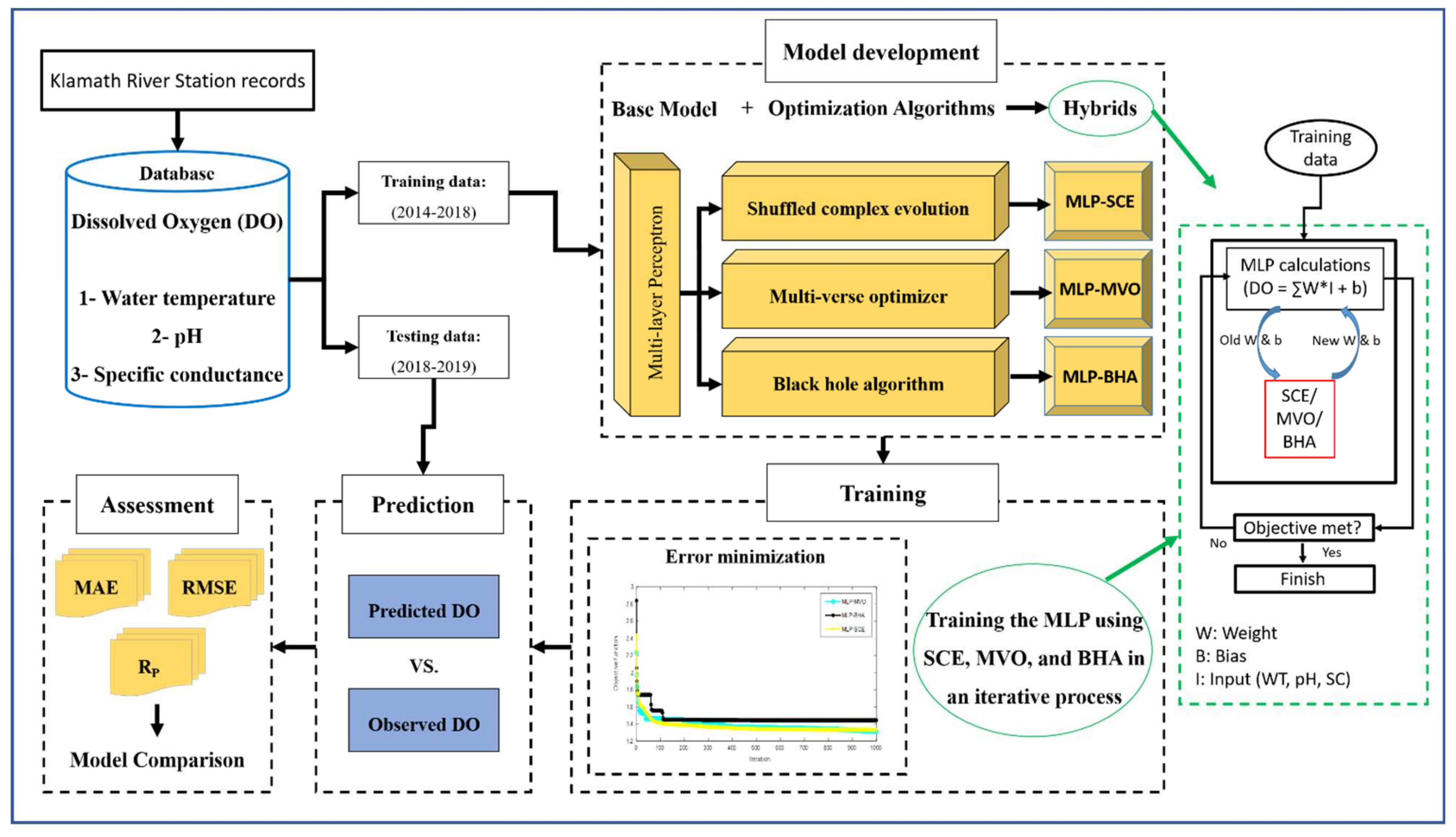
The steps of this research are shown in Figure 1. After providing the appropriate dataset, the MLP is submitted to MVO, BHA, and SCE algorithms to adjust its parameters through metaheuristic schemes. During an iterative process, the MLP is optimized to present the best possible prediction of the DO.
2.1. The MVO
As is implied by its name, the MVO is obtained from multi-verse theory in physics [75]. According to this theory, there is more than one big bang event, each of which has initiated a separate universe. The algorithm was introduced by Mirjalili et al. [76]. The main components of the MVO are wormholes, black holes, and white holes. The concepts of black and white holes run the exploration phase, while the wormhole concept is dedicated to the exploitation procedure. The pseudo code of the MVO is presented as Algorithm 1.
| Algorithm 1. Pseudo code of the MVO [77] |
| Initialize the parameters (population size, iterations, wormhole existence probability (WEP), travelling distance rate (TDR)) While maximum iteration not reached Compute the fitness for each universe AU = Sort the population BI = Normalize the fitness values for i = 2:N Black hole = i for j = 1:size(i) Generate r1 as a random value if r1 < BI(U_i) white hole = Roulette Wheel Selection(-B) U(black hole, j) = AU(white hole, j) end if Generate r2 as a random value if r2 < WEP Generate r3 and r4 as a random value if r3 < 0.5 Update the position of the universe (Equation (4)) else Update the position of the universe (Equation (4)) end if end if end for end for end while Response = Best solution. |
In the MVO, the so-called parameter of “rate of inflation” (ROI) is defined for each universe. The objects are transferred from the universes with larger ROIs to those with lower values to improve the average ROI of the whole cosmos. During an iteration, the organization of the universes is carried out with respect to their ROIs, and after a roulette wheel selection (RWS), one of them is deemed the white hole. In this relation, a set of universes can be defined as:
where g symbolizes the number of objects and k stands for the number of universes. The jth objective in the ith solution is generated according to the below equation:
where and denote upper and lower bounds, and the function produces a discrete randomly distributed number.
In each repetition, there are two options for the : (i) it is selected from earlier solutions using RWS (e.g., ∈ (, , …, ) and (ii) it does not change. It can be written as follows:
In the above equation, stands for the ith universe, gives the corresponding normalized ROI, and is a random value in [0, 1].
Equation (4) expresses the measures considered to deliver the variations of the whole universe. In this sense, the wormholes are supposed to enhance the ROI.
where signifies the jth best-fitted universe obtained so far, and , , and are random values in [0, 1]. Moreover, the two parameters of WEP and TDR stand for the wormhole existence probability and the traveling distance rate, respectively. Given Iter as the running iteration, and as the maximum number of Iters, these parameters can be calculated as follows:
where q is the accuracy of exploitation, and a and b are constant pre-defined values [78,79].
2.2. The BHA
Inspired by black hole incidents in space, Hatamlou [80] proposed the BHA in 2013. Emerging after the collapse of massive stars, a black hole is distinguished by a huge gravitational power. The stars move toward this mass, and it explains the pivotal strategy of the BHA for achieving an optimum response. A randomly generated constellation of stars represents the initial population. Based on the fitness of these stars, the most powerful one is deemed as the black hole that will absorb the surrounding ones. The pseudo code of the BHA is presented as Algorithm 2.
| Algorithm 2. Pseudo code of the BHA [81] |
| Initialize the stars xi Initialize the parameters (fitness function and iterations (Iter)) Select the best-fitted star (xb) as the black hole (BH) While maximum Iter not reached for each xi Compute the fitness if fitness (xi) > fitness (xb) xb = xi end if Update fitness and compute Equation (8) if < RBH Replace with a new star end if end for Iter = Iter + 1 end while Response = Best solution. |
In this procedure, the positions change according to the relationship below:
where rand is a random number in [0, 1], is the black hole’s position, Z is the total number of stars, and Iter symbolizes the iteration number.
Once the fitness of a star surpasses that of the black hole, they exchange their positions. In this regard, Equation (8) calculates the radius of the event horizon for the black hole.
where is the fitness of the ith star, and is the value for the black hole [82].
2.3. The SCE
Originally proposed by Duan et al. [82], the SCE has been efficiently used for dealing with optimization problems with high dimensions. The SCE can be defined as a hybrid of complex shuffling and competitive evolution concepts with the strengths of the controlled random search strategy. This algorithm (i.e., the SCE) benefits from a deterministic strategy to guide the search. Additionally, utilizing random elements has resulted in a flexible and robust algorithm. The pseudo code of the SCE is presented as Algorithm 3.
| Algorithm 3. Pseudo code of the SCE [83] |
| Initialize the population (s) Sample the population {x1, x2, …, xs} Compute the fitness (f) for each member Sort based on the obtained f values Create D0 = {xi, fi, where i = 1, 2, …, s} Create complexes W.R.T Equation (9) While maximum It not reached for q = 1:i Evolve using Competitive Complex Evolution end for Di = Di+1 end while Response = Best solution. |
The SCE is implemented in seven steps. Assuming NC as the number of complexes and NP as the number of points existing in one complex, the sample size of the algorithm is generated as S = NC × NP. In this sense, NC ≥ 1 and NP ≥ 1 + the number of design variables. Next, the samples x1, x2, …, xs are created in the viable space (i.e., within the bounds). The fitness values are also calculated using sampling distribution. In the third step, these samples are arranged with reference to their fitness. An array-like D = {xi, fi, where i = 1, 2, …, s} can be considered for storing them. This array is then divided into NC complexes (, , …, ), each of which contains NP samples (Equation (9))
In the fifth step, each complex is evolved by the competitive complex evolution algorithm. Later, in a process named the shuffling of the complexes, all complexes are replaced in array D. This array is then sorted based on the fitness values. Lastly, the algorithm checks for stopping criteria that terminate the process [84].
2.4. Accuracy Criteria
The quality of the results is lastly evaluated using Pearson’s correlation coefficient (RP) along with mean absolute error (MAE) and RMSE. They analyze the agreement and difference between the observed and predicted values of a target parameter. In the present work, given and as the predicted and observed DOs, the RP, MAE, and RMSE are expressed by the following equations:
where K signifies the number of compared pairs.
3. Data
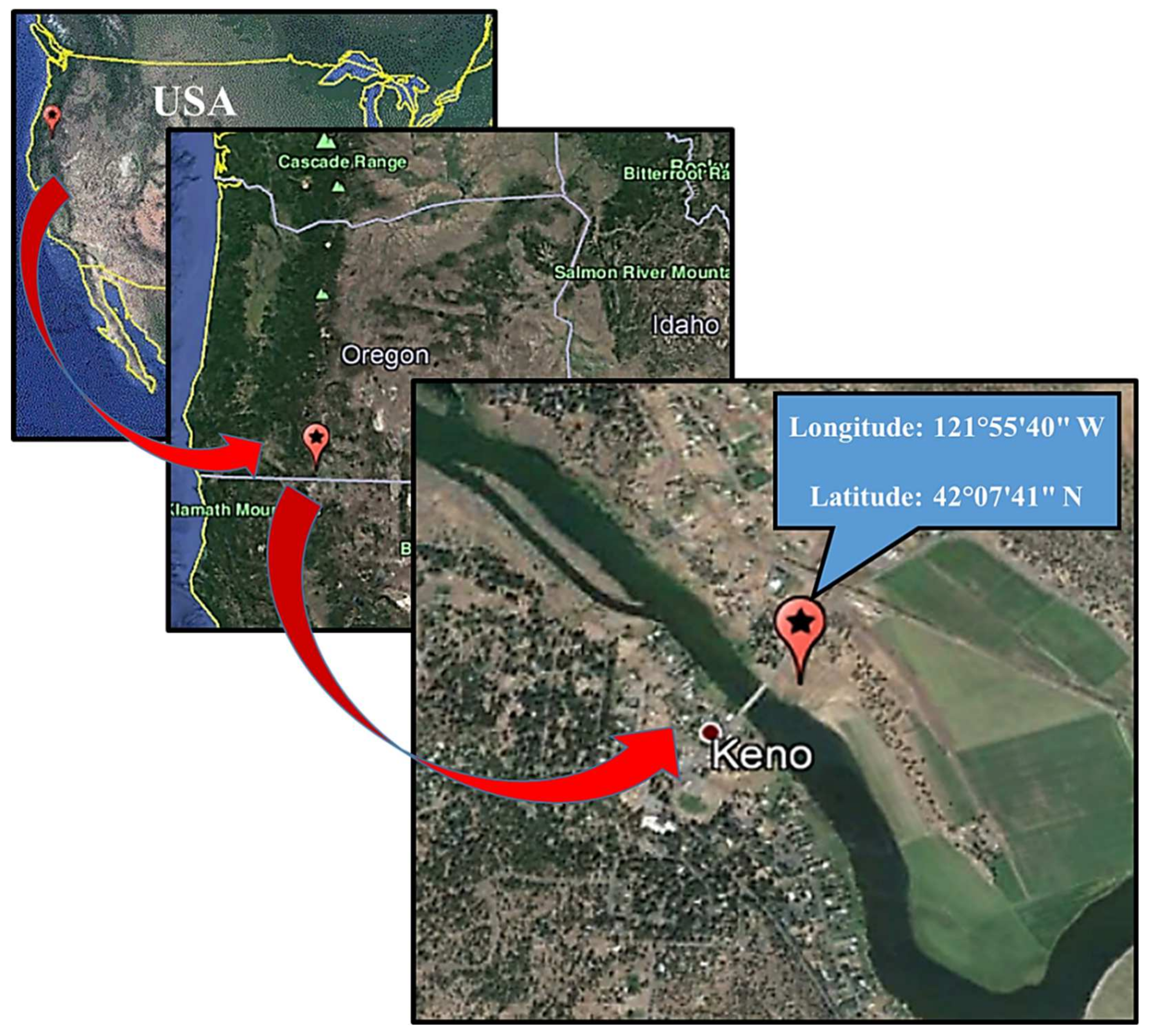
As a matter of fact, intelligent models should first learn the pattern of the intended parameter in order to predict it. This learning process is carried out by analyzing the dependence of the target parameter on some independent factors. In this work, DO is the target parameter for water temperature (WT), pH, and specific conductance (SC). This study uses the data belonging to a US Geological Survey (USGS) station, namely, the Klamath River (station number: 11509370). As Figure 2 illustrates, this station is located in Klamath County, Oregon State.
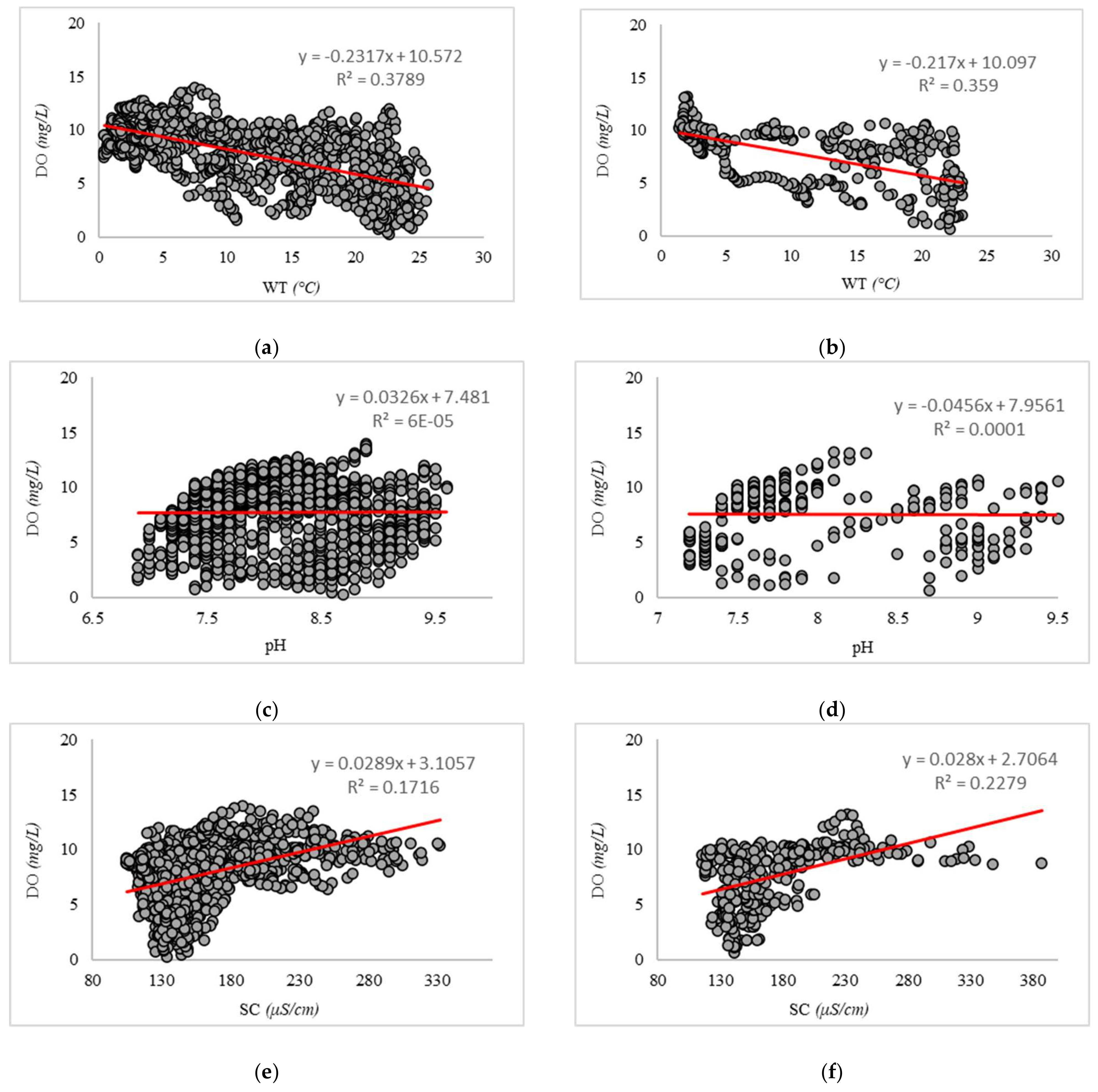
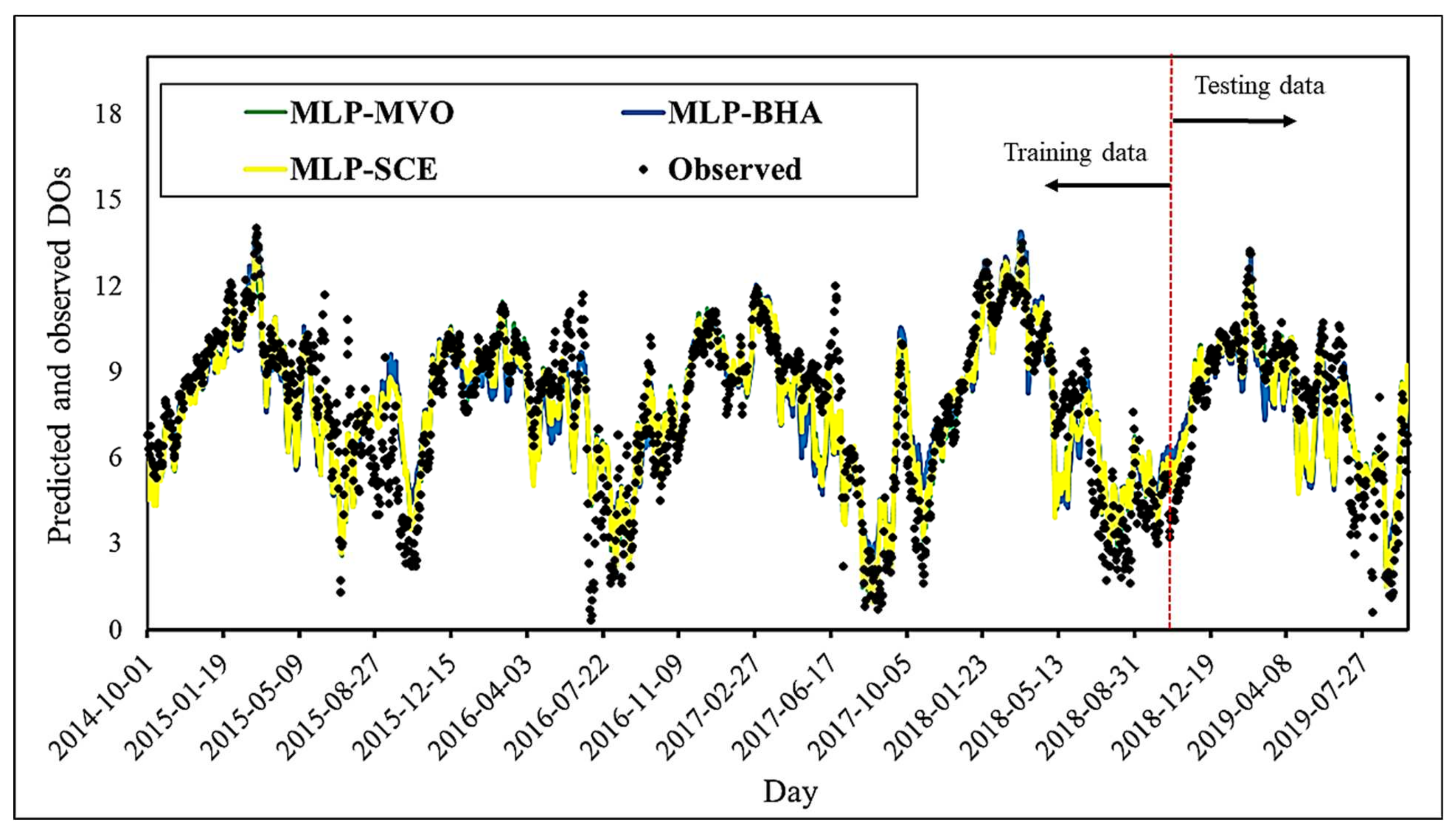
Pattern recognition is fulfilled by means of data obtained between 1 October 2014 and 30 September 2018. After training the models, the DO for the subsequent year (i.e., from 1 October 2018 to 30 September 2019) is predicted. Since the models do not know this data, the accuracy of this process will reflect their capability to predict DO in unseen conditions. Hereafter, these two groups are categorized as training data and testing data, respectively. Figure 3 depicts DO vs. WT, PH, and SC for the (a, c, and e) training and (b, d, and f) testing data. Based on the available data for the mentioned periods, the training and testing groups contain 1430 and 352 records, respectively. Moreover, the statistical description of these datasets is presented in Table 1
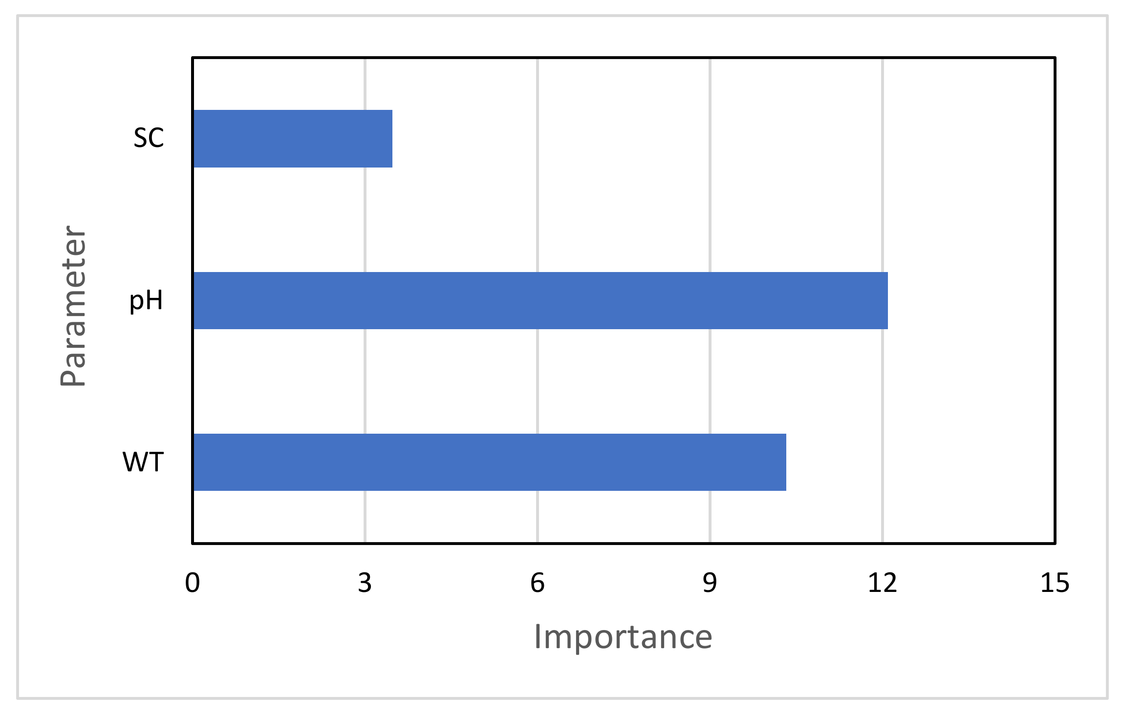
Moreover, the effect of the inputs on DO is investigated using a tree-based ensemble method. To do this, a bagged ensemble of 200 regression trees is implemented, and the outcome is reported as a value of importance. Figure 4 shows the results. As can be seen, SC is smaller than WT and the effect of WT smaller than pH. In other words, pH has the greatest impact on DO concentration in this case.
4. Results and Discussion
4.1. Optimization and Weight Adjustment
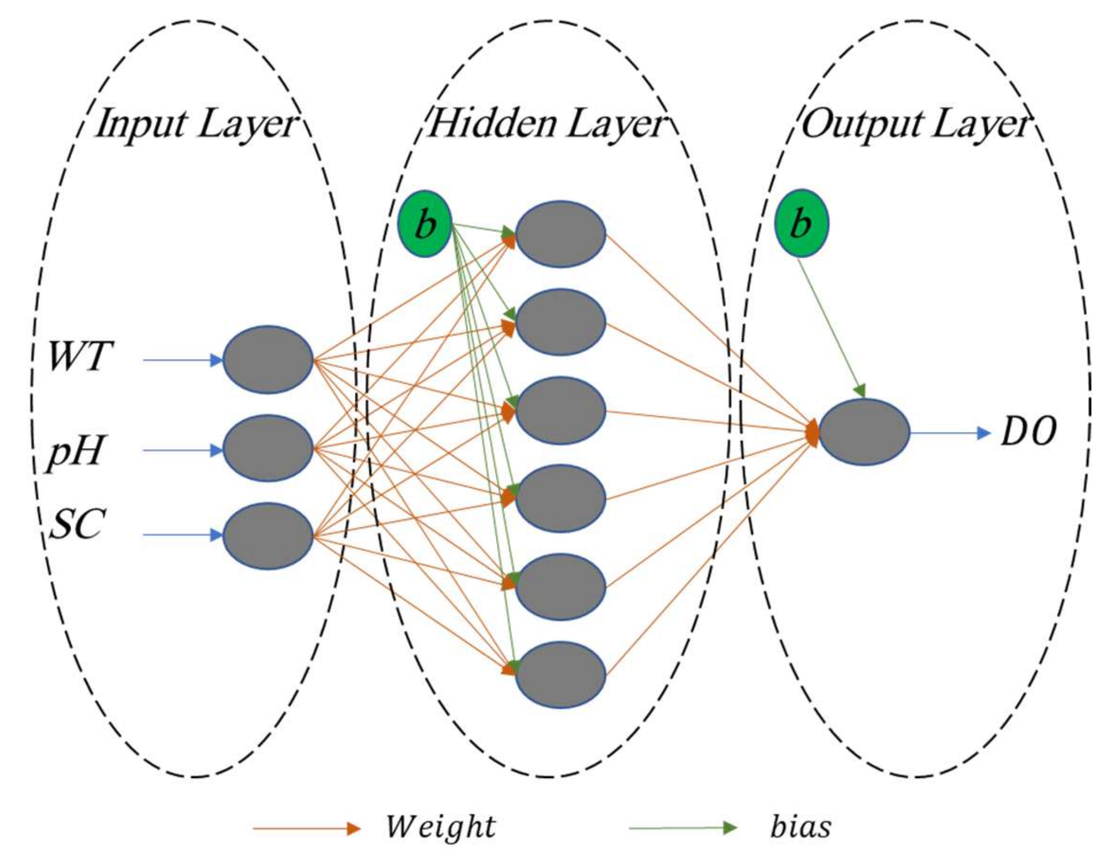
As explained, the proposed hybrid models are designed in the way that MVO, BHA, and SCE algorithms are responsible for adjusting the weights and biases of the MLP. To do this, a raw MLP structure (that wants to predict DO from WT, pH, and SC) should be given as the optimization problem to the mentioned algorithms. In this work, a three-layered MLP with three neurons in the input layer (each for one input), six neurons in the middle layer, and one neuron (for DO) in the last layer was considered, noting that the value of 6 was determined after a trial and error process; this is schematically shown in Figure 5.
The overall formulation of a neuron can be expressed as follows:
where f(x) is the activation function used by the neurons in a layer; additionally, RN and IN denote the response and input of the neuron N, respectively. With a large number of these equations, each algorithm first suggests a stochastic response for the W and b values. In the next iterations, the algorithms improve this response in order to build a more accurate MLP. The formulation of a trained MLP network is presented at the end of the study to better illustrate this concept.
RN = f(IN × W + b)
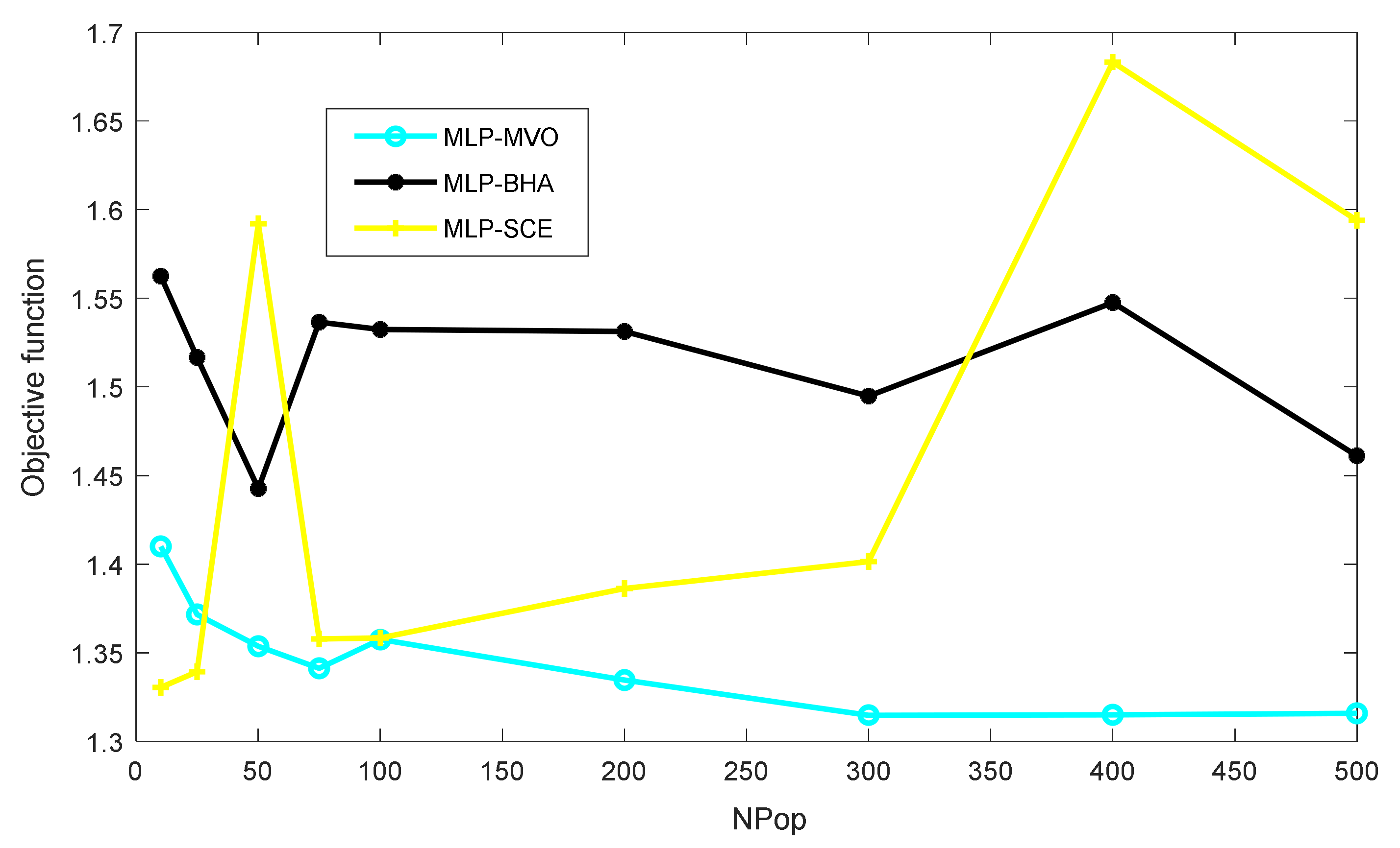
The created hybrids are implemented with different population sizes (NPops) of the trainer algorithm to achieve the best results. Figure 6 shows the values of the objective function obtained for the NPops of 10, 25, 50, 75, 100, 200, 300, 400, and 500. In the case of this study, the objective function is reported by the RMSE criterion. Figure 6 shows that unlike the SCE, which gives more quality training with small NPops, the MVO performs better with the three largest NPops. The BHA, however, did not show any specific behavior. Overall, the MVO, BHA, and SCE with the NPops of 300, 50, and 10, respectively, could adjust the MLP parameters with the lowest error.
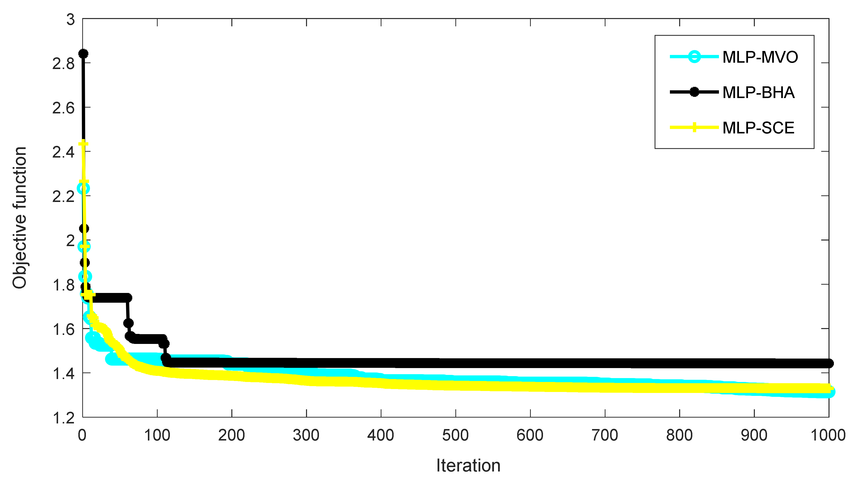
As stated, metaheuristic algorithms minimize the errors in an iterative process. Figure 7 shows the convergence curve plotted for the selected configurations of the MLP-MVO, BHA-MVO, and SCE-MVO. To this end, the training RMSE is calculated for a total of 1000 iterations. According to Figure 7, the optimum values of the objective function are 1.314816444, 1.442582978, and 1.33041779 for the MLP-MVO, BHA-MVO, and SCE-MVO, respectively. These configurations are applied in the next section to predict DO. Their results are then evaluated for accuracy assessment.
4.2. Assessment of the Results
Figure 8 shows a comparison between the observed DO rates and those predicted by the MLP-MVO, MLP-BHA, and MLP-SCE for the whole five years. At a glance, all three models could properly capture DO behavior. It indicates that the algorithms have designated appropriate weights for each input parameter (WT, PH, and SC). The results of the training and testing datasets are presented in detail in the following figure.
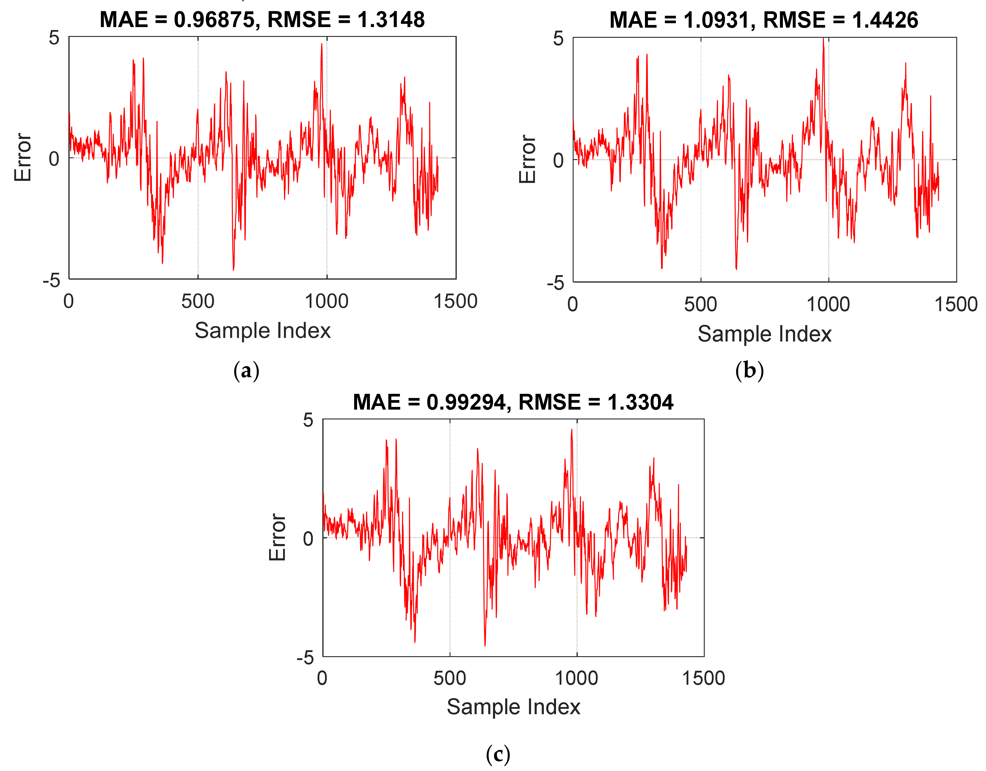
Focusing on the training results, an acceptable level of accuracy is reflected by the RMSEs of 1.3148, 1.4426, and 1.3304 for the MLP-MVO, MLP-BHA, and MLP-SCE. In this sense, the values of the MAE (0.9687, 1.0931, and 0.9929) confirmed this statement and showed that all three models had understood the DO pattern with good accuracy. By comparison, it can be deduced that both error values of the MLP-MVO are lower than the two other models. Based on the same reason, the MLP-SCE outperformed the MLP-BHA.
Figure 9 depicts the errors obtained for the training data. This value is calculated as the difference between the predicted and observed DOs. The errors of the MLP-MVO, MLP-BHA, and MLP-SCE have the following ranges: [−4.6396, 4.7003], [−4.4964, 4.9537], and [−4.5585, 4.5653].
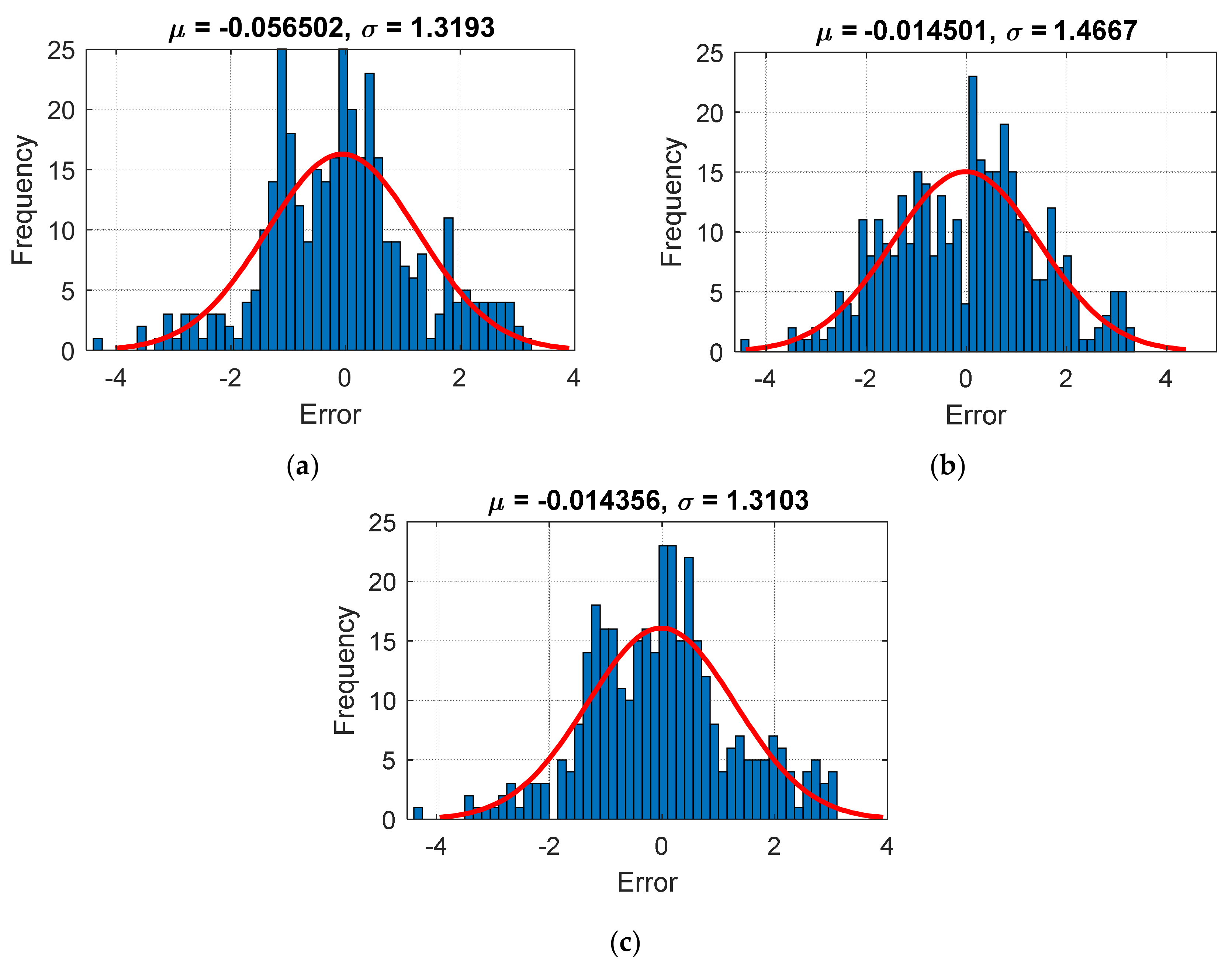
As stated previously, the quality of the testing results shows how successful a trained model can be in confronting new conditions. The data of the fifth year were considered as these conditions in this study. Figure 10 depicts the histogram of the testing errors. In these charts, µ stands for the mean error, and σ represents the standard error. In this phase, the RMSEs of 1.3187, 1.4647, and 1.3085, along with the MEAs of 1.0161, 1.1997, and 1.0122, imply the power of the used models for dealing with strange data. It means that the weights (and biases) determined in the previous section have successfully mapped the relationship between DO and WT, PH, and SC for the second phase. From the comparison point of view, unlike the training phase, the SCE-based hybrid outperformed the MLP-MVO. The MLP-BHA, however, presented the poorest prediction of DO, again.
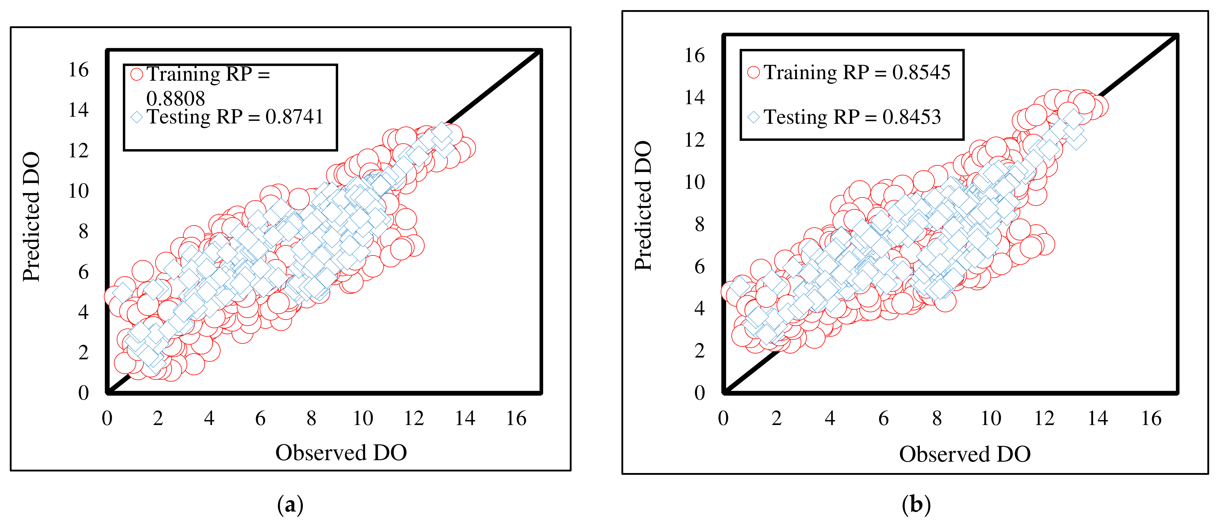
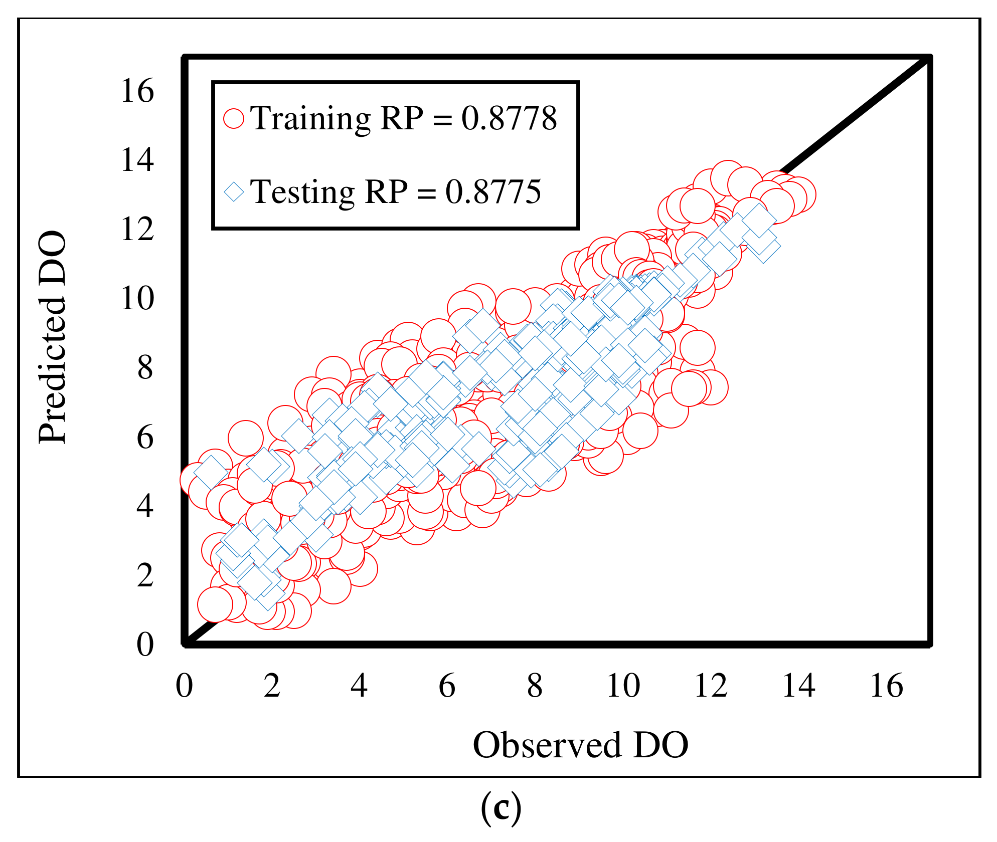
The third accuracy indicator (i.e., the RP) shows the agreement between the predicted and observed DO rates. This index can range within [−1, +1], where −1 (+1) indicates a totally negative (positive) correlation, and 0 means no correlation. Figure 11 shows a scatterplot for each model containing both training and testing results. As can be seen, all outputs are positively aggregated around the best-fit line (i.e., the black line). For the training results, the RPs of 0.8808, 0.8545, and 0.8778 indicate the higher consistency of the MLP-MVO results, while the values of 0.8741, 0.8453, and 0.8775 demonstrate the superiority of the MLP-SCE in the testing phase.
4.3. Cross-Validation
In order to further verify the potential of the implemented models, the trained models (i.e., the MVO, BHA, and SCE, with the NPops of 300, 50, and 10, respectively) are applied to another station called Fanno Creek (station number: 14206950). Similar to Klamath River, it is located in the Oregon State but in the northern part (longitude: 122°45′13″ W and latitude: 45°24′13″ N). The models predicted the DO for the water year 2019 using the daily records of WT, SC, and pH. Notably, the measured DO ranged from 5.40 to 13.20 mg/L in this site.
The results are shown in Table 2. As can be seen, the performance of all three models is satisfying, and the predicted values are well-correlated with the observed DO rates. It professes that the models can be used for new prediction cases. However, the combination of inputs (i.e., taking WT, pH, and SC into account) should be respected for all study cases.
4.4. Further Discussion
Due to the water quality situation in the Klamath River, this study was dedicated to suggesting novel predictive tools for analyzing the DO concentration in this reach. Notably, this river is important for irrigation, flows, and hydropower generation [72]. It was discussed that DO should be evaluated in response to different key parameters. Another difficulty is that the DO does not follow a certain pattern over time. Hence, it is necessary to tackle these complexities by selecting appropriate models.
Many scholars have stated their tendency regarding the use of hybrid methods for similar issues (e.g., sediment concentration [85] and salinity [86] predictions). The reason for the development of such models can be the use of an optimization technique in the position of a trainer algorithm. In the case of DO modeling in this study, each of the MVO, BHA, and SCE algorithms drove an MLP neural network. In other words, their specific solutions were employed to analyze the relationship between DO and influential parameters through a neural framework.
The high level of accuracy achieved shows that DO can be promisingly predicted. However, there are some suggestions that should be applied for even more efficient solutions. The first part is related to methodology. Optimization using metaheuristic techniques needs to be carefully monitored to select appropriate parameters. For example, the number of iterations and the complexity of the population are better optimized vs. time, where time is as important as accuracy. However, the focus of this study was mostly on the accuracy of prediction (Figure 6). Another idea in this regard can be to test different metaheuristic techniques to find the quickest [87]. Another potential idea would be conducting comparisons with benchmark machine learning solutions such as the ANFIS and SVR as well as their hybridized versions.
The dataset is also a key item. The factors that can be regarded are optimizing the number of input parameters, selecting the appropriate time period, and the pre-processing and purification of misleading samples, among others. In this work, a valid 5-year dataset with three inputs was used, and the results showed that it could provide sufficient samples to be analyzed by the algorithms. Since the models could predict the DO of the testing period without prior knowledge of it, they can be used for further unseen events. Additionally, these results were achieved with the effect of only three influential parameters. Such simplicity is effective for avoiding complicated simulations and reducing the cost of computations.
4.5. SCE-Based Formula
In this section, the formulation of the MLP-SCE model is presented due to its superiority in the prediction phase as well as a simpler configuration compared to the MVO and BHA. Moreover, considering time efficiency, the SCE could optimize the ANN in a meaningfully shorter time. The elapsed times were approximately 5980, 675, and 531 s for the selected configurations of the MLP-MVO, MLP-BHA, and MLP-SCE, respectively (under a core i7 (at 1.8 GHz) operating system with 16 gigs of RAM).
This formula can serve as a predictive equation that estimates DO for given values of WT, pH, and SC. This model predicts DO based on Equation (14), in which Input stands for three inputs, and IW and b1 are their corresponding weights and bias vectors, respectively. LW and b2 symbolize the same values but for the output layer (Figure 5). These numbers are optimally tuned by the SCE for the MLP so that the lowest training error is achieved (Figure 7). Additionally, f(x) (i.e., the activation function) is presented in Equation (20). It is worth noting that due to the neural network mechanism, this formula must be fed with normalized data.
DO = [LW] × (f (([IW] × [Input]) + [b1])) + [b2]
5. Conclusions
This research points out the suitability of metaheuristic strategies for analyzing the relationship between DO and three influential factors (WT, PH, and SC) through the principles of a multi-layer perceptron network. The algorithms used were multi-verse optimizer, black hole algorithm, and shuffled complex evolution, which showed high applicability for optimization objectives. A finding of this study was that while the MVO needs NPop = 300 to give proper training to the MLP, two other algorithms can do this with smaller populations (NPops of 50 and 10). According to the findings of the training phase, the MVO can achieve a more profound understanding of the mentioned relationship. The RMSE of this model was 1.3148, which was found to be smaller than MLP-BHA (1.4426) and MLP-SCE (1.3304). However, different results were observed in the testing phase. The SCE-based model came up with the largest accuracy (the RPs were 0.8741, 0.8453, and 0.8775). All in all, the authors believe that the tested models can serve as promising ways for predicting DO. However, assessing other metaheuristic techniques and other hybridization strategies is recommended for future studies.
Author Contributions
F.Y., writing—review and editing, visualization, supervision; H.M., methodology, software validation, writing—original draft preparation; A.M., writing—review and editing, visualization, supervision, project administration. All authors have read and agreed to the published version of the manuscript.
Funding
This research received no external funding.
Institutional Review Board Statement
Not applicable.
Informed Consent Statement
Not applicable.
Data Availability Statement
Not applicable.
Conflicts of Interest
The authors declare no conflict of interest.
Abbreviations
| DO | Dissolved oxygen |
| SVR | Support vector regression |
| ANN | Artificial neural networks |
| MLP | Multi-layer perceptron |
| RBF | Radial basis function |
| GRNN | General regression neural network |
| ANFIS | Adaptive neuro-fuzzy inference system |
| GA | Genetic algorithm |
| SFLA | Shuffled frog leaping algorithm |
| FOA | Fruit fly optimization |
| PSO | Particle swarm optimization |
| MVO | Multi-verse optimizer |
| BHA | Black hole algorithm |
| SCE | Shuffled complex evolution |
| MLR | Multiple linear regression |
| RNN | Recurrent neural network |
| ROI | Rate of inflation |
| RWS | Roulette wheel selection |
| RP | Pearson’s correlation coefficient |
| MAE | Mean absolute error |
| RMSE | Root mean square error |
| WT | Water temperature |
| SC | Specific conductance |
References
- Kisi, O.; Alizamir, M.; Gorgij, A.D. Dissolved oxygen prediction using a new ensemble method. Environ. Sci. Pollut. Res. 2020, 27, 9589–9603. [Google Scholar] [CrossRef] [PubMed]
- Liu, S.; Yan, M.; Tai, H.; Xu, L.; Li, D. Prediction of dissolved oxygen content in aquaculture of Hyriopsis cumingii using Elman neural network. In Proceedings of the International Conference on Computer and Computing Technologies in Agriculture, Beijing, China, 29–31 October 2011; Springer: Berlin/Heidelberg, Germany, 2011; pp. 508–518. [Google Scholar]
- Heddam, S.; Kisi, O. Extreme learning machines: A new approach for modeling dissolved oxygen (DO) concentration with and without water quality variables as predictors. Environ. Sci. Pollut. Res. 2017, 24, 16702–16724. [Google Scholar] [CrossRef]
- Li, C.; Li, Z.; Wu, J.; Zhu, L.; Yue, J. A hybrid model for dissolved oxygen prediction in aquaculture based on multi-scale features. Inf. Process. Agric. 2018, 5, 11–20. [Google Scholar] [CrossRef]
- Ay, M.; Kisi, O. Modeling of Dissolved Oxygen Concentration Using Different Neural Network Techniques in Foundation Creek, El Paso County, Colorado. J. Environ. Eng. 2012, 138, 654–662. [Google Scholar] [CrossRef]
- Elkiran, G.; Nourani, V.; Abba, S.; Abdullahi, J. Artificial intelligence-based approaches for multi-station modelling of dissolve oxygen in river. Glob. J. Environ. Sci. Manag. 2018, 4, 439–450. [Google Scholar]
- Zhang, M.; Zhang, L.; Tian, S.; Zhang, X.; Guo, J.; Guan, X.; Xu, P. Effects of graphite particles/Fe3+ on the properties of anoxic activated sludge. Chemosphere 2020, 253, 126638. [Google Scholar] [CrossRef] [PubMed]
- Sun, M.; Hou, B.; Wang, S.; Zhao, Q.; Zhang, L.; Song, L.; Zhang, H. Effects of NaClO shock on MBR performance under continuous operating conditions. Environ. Sci. Water Res. Technol. 2021, 7, 396–404. [Google Scholar] [CrossRef]
- Zhao, C.; Li, J. Equilibrium Selection under the Bayes-Based Strategy Updating Rules. Symmetry 2020, 12, 739. [Google Scholar] [CrossRef]
- Liu, M.; Xue, Z.; Zhang, H.; Li, Y. Dual-channel membrane capacitive deionization based on asymmetric ion adsorption for continuous water desalination. Electrochem. Commun. 2021, 125, 106974. [Google Scholar] [CrossRef]
- Yang, Y.; Li, Y.; Yao, J.; Iglauer, S.; Luquot, L.; Zhang, K.; Sun, H.; Zhang, L.; Song, W.; Wang, Z. Dynamic Pore-Scale Dissolution by CO2-Saturated Brine in Carbonates: Impact of Homogeneous Versus Fractured Versus Vuggy Pore Structure. Water Resour. Res. 2020, 56, 26112. [Google Scholar] [CrossRef]
- Zhao, X.; Gu, B.; Gao, F.; Chen, S. Matching Model of Energy Supply and Demand of the Integrated Energy System in Coastal Areas. J. Coast. Res. 2020, 103, 983–989. [Google Scholar] [CrossRef]
- Zuo, X.; Dong, M.; Gao, F.; Tian, S. The Modeling of the Electric Heating and Cooling System of the Integrated Energy System in the Coastal Area. J. Coast. Res. 2020, 103, 1022–1029. [Google Scholar] [CrossRef]
- Liu, J.; Yi, Y.; Wang, X. Exploring factors influencing construction waste reduction: A structural equation modeling approach. J. Clean. Prod. 2020, 276, 123185. [Google Scholar] [CrossRef]
- Gao, N.; Wang, B.; Lu, K.; Hou, H. Complex band structure and evanescent Bloch wave propagation of periodic nested acoustic black hole phononic structure. Appl. Acoust. 2021, 177, 107906. [Google Scholar] [CrossRef]
- Liu, J.; Liu, Y.; Wang, X. An environmental assessment model of construction and demolition waste based on system dynamics: A case study in Guangzhou. Environ. Sci. Pollut. Res. 2019, 27, 37237–37259. [Google Scholar] [CrossRef] [PubMed]
- Zuo, C.; Chen, Q.; Tian, L.; Waller, L.; Asundi, A. Transport of intensity phase retrieval and computational imaging for partially coherent fields: The phase space perspective. Opt. Lasers Eng. 2015, 71, 20–32. [Google Scholar] [CrossRef]
- Zuo, C.; Sun, J.; Jialin, Z.; Zhang, J.; Asundi, A.; Chen, Q. High-resolution transport-of-intensity quantitative phase microscopy with annular illumination. Sci. Rep. 2017, 7, 1–22. [Google Scholar] [CrossRef]
- Zhang, L.; Zheng, J.; Tian, S.; Zhang, H.; Guan, X.; Zhu, S.; Zhang, X.; Bai, Y.; Xu, P.; Zhang, J.; et al. Effects of Al3+ on the microstructure and bioflocculation of anoxic sludge. J. Environ. Sci. 2020, 91, 212–221. [Google Scholar] [CrossRef]
- Hong, X.-C.; Wang, G.-Y.; Liu, J.; Song, L.; Wu, E.T. Modeling the impact of soundscape drivers on perceived birdsongs in urban forests. J. Clean. Prod. 2021, 292, 125315. [Google Scholar] [CrossRef]
- Zhang, W.; Hu, Y.; Liu, J.; Wang, H.; Wei, J.; Sun, P.; Wu, L.; Zheng, H. Progress of ethylene action mechanism and its application on plant type formation in crops. Saudi J. Biol. Sci. 2020, 27, 1667–1673. [Google Scholar] [CrossRef]
- Han, C.; Zhang, B.; Chen, H.; Wei, Z.; Liu, Y. Spatially distributed crop model based on remote sensing. Agric. Water Manag. 2019, 218, 165–173. [Google Scholar] [CrossRef]
- Qiao, W.; Wang, Y.; Zhang, J.; Tian, W.; Tian, Y.; Yang, Q. An innovative coupled model in view of wavelet transform for predicting short-term PM10 concentration. J. Environ. Manag. 2021, 289, 112438. [Google Scholar] [CrossRef]
- Seyedashraf, O.; Mehrabi, M.; Akhtari, A.A. Novel approach for dam break flow modeling using computational intelligence. J. Hydrol. 2018, 559, 1028–1038. [Google Scholar] [CrossRef]
- Moayedi, H.; Mehrabi, M.; Mosallanezhad, M.; Rashid, A.S.A.; Pradhan, B. Modification of landslide susceptibility mapping using optimized PSO-ANN technique. Eng. Comput. 2019, 35, 967–984. [Google Scholar] [CrossRef]
- Xu, Y.; Chen, H.; Luo, J.; Zhang, Q.; Jiao, S.; Zhang, X. Enhanced Moth-flame optimizer with mutation strategy for global optimization. Inf. Sci. 2019, 492, 181–203. [Google Scholar] [CrossRef]
- Xia, J.; Chen, H.; Li, Q.; Zhou, M.; Chen, L.; Cai, Z.; Fang, Y.; Zhou, H. Ultrasound-based differentiation of malignant and benign thyroid Nodules: An extreme learning machine approach. Comput. Methods Programs Biomed. 2017, 147, 37–49. [Google Scholar] [CrossRef]
- Wang, M.; Chen, H.; Yang, B.; Zhao, X.; Hu, L.; Cai, Z.; Huang, H.; Tong, C. Toward an optimal kernel extreme learning machine using a chaotic moth-flame optimization strategy with applications in medical diagnoses. Neurocomputing 2017, 267, 69–84. [Google Scholar] [CrossRef]
- Chen, H.-L.; Wang, G.; Ma, C.; Cai, Z.-N.; Liu, W.-B.; Wang, S.-J. An efficient hybrid kernel extreme learning machine approach for early diagnosis of Parkinson׳s disease. Neurocomputing 2016, 184, 131–144. [Google Scholar] [CrossRef] [Green Version]
- Xu, X.; Chen, H.-L. Adaptive computational chemotaxis based on field in bacterial foraging optimization. Soft Comput. 2013, 18, 797–807. [Google Scholar] [CrossRef]
- Zhao, D.; Liu, L.; Yu, F.; Heidari, A.A.; Wang, M.; Liang, G.; Muhammad, K.; Chen, H. Chaotic random spare ant colony optimization for multi-threshold image segmentation of 2D Kapur entropy. Knowl.-Based Syst. 2021, 216, 106510. [Google Scholar] [CrossRef]
- Zhao, X.; Li, D.; Yang, B.; Ma, C.; Zhu, Y.; Chen, H. Feature selection based on improved ant colony optimization for online detection of foreign fiber in cotton. Appl. Soft Comput. 2014, 24, 585–596. [Google Scholar] [CrossRef]
- Moayedi, H.; Mehrabi, M.; Kalantar, B.; Mu’Azu, M.A.; Rashid, A.S.A.; Foong, L.K.; Nguyen, H. Novel hybrids of adaptive neuro-fuzzy inference system (ANFIS) with several metaheuristic algorithms for spatial susceptibility assessment of seismic-induced landslide. Geomat. Nat. Hazards Risk 2019, 10, 1879–1911. [Google Scholar] [CrossRef] [Green Version]
- Chen, H.; Heidari, A.A.; Chen, H.; Wang, M.; Pan, Z.; Gandomi, A.H. Multi-population differential evolution-assisted Harris hawks optimization: Framework and case studies. Future Gener. Comput. Syst. 2020, 111, 175–198. [Google Scholar] [CrossRef]
- Zhang, Y.; Liu, R.; Wang, X.; Chen, H.; Li, C. Boosted binary Harris hawks optimizer and feature selection. Eng. Comput. 2020, 25, 1–30. [Google Scholar] [CrossRef]
- Zhao, X.; Zhang, X.; Cai, Z.; Tian, X.; Wang, X.; Huang, Y.; Chen, H.; Hu, L. Chaos enhanced grey wolf optimization wrapped ELM for diagnosis of paraquat-poisoned patients. Comput. Biol. Chem. 2019, 78, 481–490. [Google Scholar] [CrossRef] [PubMed]
- Hu, J.; Chen, H.; Heidari, A.A.; Wang, M.; Zhang, X.; Chen, Y.; Pan, Z. Orthogonal learning covariance matrix for defects of grey wolf optimizer: Insights, balance, diversity, and feature selection. Knowl.-Based Syst. 2021, 213, 106684. [Google Scholar] [CrossRef]
- Zhang, Y.; Liu, R.; Heidari, A.A.; Wang, X.; Chen, Y.; Wang, M.; Chen, H. Towards augmented kernel extreme learning models for bankruptcy prediction: Algorithmic behavior and comprehensive analysis. Neurocomputing 2021, 430, 185–212. [Google Scholar] [CrossRef]
- Tu, J.; Chen, H.; Liu, J.; Heidari, A.A.; Zhang, X.; Wang, M.; Ruby, R.; Pham, Q.-V. Evolutionary biogeography-based whale optimization methods with communication structure: Towards measuring the balance. Knowl.-Based Syst. 2021, 212, 106642. [Google Scholar] [CrossRef]
- Shan, W.; Qiao, Z.; Heidari, A.A.; Chen, H.; Turabieh, H.; Teng, Y. Double adaptive weights for stabilization of moth flame optimizer: Balance analysis, engineering cases, and medical diagnosis. Knowl.-Based Syst. 2021, 214, 106728. [Google Scholar] [CrossRef]
- Yu, H.; Li, W.; Chen, C.; Liang, J.; Gui, W.; Wang, M.; Chen, H. Dynamic Gaussian bare-bones fruit fly optimizers with abandonment mechanism: Method and analysis. Eng. Comput. 2020, 1–29. [Google Scholar] [CrossRef]
- Hu, L.; Hong, G.; Ma, J.; Wang, X.; Chen, H. An efficient machine learning approach for diagnosis of paraquat-poisoned patients. Comput. Biol. Med. 2015, 59, 116–124. [Google Scholar] [CrossRef]
- Shen, L.; Chen, H.; Yu, Z.; Kang, W.; Zhang, B.; Li, H.; Yang, B.; Liu, D. Evolving support vector machines using fruit fly optimization for medical data classification. Knowl.-Based Syst. 2016, 96, 61–75. [Google Scholar] [CrossRef]
- Wang, M.; Chen, H. Chaotic multi-swarm whale optimizer boosted support vector machine for medical diagnosis. Appl. Soft Comput. 2020, 88, 105946. [Google Scholar] [CrossRef]
- Li, C.; Hou, L.; Sharma, B.Y.; Li, H.; Chen, C.; Li, Y.; Zhao, X.; Huang, H.; Cai, Z.; Chen, H. Developing a new intelligent system for the diagnosis of tuberculous pleural effusion. Comput. Methods Programs Biomed. 2018, 153, 211–225. [Google Scholar] [CrossRef] [PubMed]
- Liu, Z.; Gilbert, G.; Cepeda, J.M.; Lysdahl, A.O.K.; Piciullo, L.; Hefre, H.; Lacasse, S. Modelling of shallow landslides with machine learning algorithms. Geosci. Front. 2021, 12, 385–393. [Google Scholar] [CrossRef]
- Csábrági, A.; Molnár, S.; Tanos, P.; Kovács, J. Application of artificial neural networks to the forecasting of dissolved oxygen content in the Hungarian section of the river Danube. Ecol. Eng. 2017, 100, 63–72. [Google Scholar] [CrossRef]
- Csábrági, A.; Molnár, S.; Tanos, P.; Kovács, J.; Molnár, M.; Szabó, I.; Hatvani, I.G. Estimation of dissolved oxygen in riverine ecosystems: Comparison of differently optimized neural networks. Ecol. Eng. 2019, 138, 298–309. [Google Scholar] [CrossRef]
- Heddam, S. Simultaneous modelling and forecasting of hourly dissolved oxygen concentration (DO) using radial basis function neural network (RBFNN) based approach: A case study from the Klamath River, Oregon, USA. Model. Earth Syst. Environ. 2016, 2, 1–18. [Google Scholar] [CrossRef] [Green Version]
- Heddam, S. Fuzzy Neural Network (EFuNN) for Modelling Dissolved Oxygen Concentration (DO). In Intelligence Systems in Environmental Management: Theory and Applications; Springer: Berlin/Heidelberg, Germany, 2017; pp. 231–253. [Google Scholar]
- Khan, U.T.; Valeo, C. Dissolved oxygen prediction using a possibility theory based fuzzy neural network. Hydrol. Earth Syst. Sci. 2016, 20, 2267–2293. [Google Scholar] [CrossRef] [Green Version]
- Ahmed, A.M.; Shah, S.M.A. Application of adaptive neuro-fuzzy inference system (ANFIS) to estimate the biochemical oxygen demand (BOD) of Surma River. J. King Saud Univ. Eng. Sci. 2017, 29, 237–243. [Google Scholar] [CrossRef] [Green Version]
- Heddam, S. Modeling hourly dissolved oxygen concentration (DO) using two different adaptive neuro-fuzzy inference systems (ANFIS): A comparative study. Environ. Monit. Assess. 2014, 186, 597–619. [Google Scholar] [CrossRef] [PubMed]
- Ranković, V.; Radulović, J.; Radojevic, I.; Ostojić, A.; Čomić, L. Prediction of dissolved oxygen in reservoirs using adaptive network-based fuzzy inference system. J. Hydroinform. 2011, 14, 167–179. [Google Scholar] [CrossRef]
- Heddam, S.; Kisi, O. Modelling daily dissolved oxygen concentration using least square support vector machine, multivariate adaptive regression splines and M5 model tree. J. Hydrol. 2018, 559, 499–509. [Google Scholar] [CrossRef]
- Kisi, O.; Akbari, N.; Sanatipour, M.; Hashemi, A.; Teimourzadeh, K.; Shiri, J. Modeling of Dissolved Oxygen in River Water Using Artificial Intelligence Techniques. J. Environ. Inform. 2013, 22. [Google Scholar] [CrossRef]
- Li, X.; Sha, J.; Wang, Z.-L. A comparative study of multiple linear regression, artificial neural network and support vector machine for the prediction of dissolved oxygen. Hydrol. Res. 2016, 48, 1214–1225. [Google Scholar] [CrossRef]
- Antanasijević, D.; Pocajt, V.; Pericgrujic, A.A.; Ristić, M. Modelling of dissolved oxygen in the Danube River using artificial neural networks and Monte Carlo Simulation uncertainty analysis. J. Hydrol. 2014, 519, 1895–1907. [Google Scholar] [CrossRef]
- Ouma, Y.O.; Okuku, C.O.; Njau, E.N. Use of Artificial Neural Networks and Multiple Linear Regression Model for the Prediction of Dissolved Oxygen in Rivers: Case Study of Hydrographic Basin of River Nyando, Kenya. Complexity 2020, 2020, 9570789. [Google Scholar] [CrossRef]
- Zhang, Y.-F.; Fitch, P.; Thorburn, P.J. Predicting the Trend of Dissolved Oxygen Based on the kPCA-RNN Model. Water 2020, 12, 585. [Google Scholar] [CrossRef] [Green Version]
- Ali, S.A.; Parvin, F.; Vojteková, J.; Costache, R.; Linh, N.T.T.; Pham, Q.B.; Vojtek, M.; Gigović, L.; Ahmad, A.; Ghorbani, M.A. GIS-based landslide susceptibility modeling: A comparison between fuzzy multi-criteria and machine learning algorithms. Geosci. Front. 2021, 12, 857–876. [Google Scholar] [CrossRef]
- Ahmed, M.H. Prediction of the Concentration of Dissolved Oxygen in Running Water by Employing A Random Forest Machine Learning Technique. J. Hydrol. 2021. [Google Scholar] [CrossRef]
- Ay, M.; Kişi, Ö. Estimation of dissolved oxygen by using neural networks and neuro fuzzy computing techniques. J. Civil Eng. 2017, 21, 1631–1639. [Google Scholar] [CrossRef]
- Rajaee, T.; Khani, S.; Ravansalar, M. Artificial intelligence-based single and hybrid models for prediction of water quality in rivers: A review. Chemom. Intell. Lab. Syst. 2020, 200, 103978. [Google Scholar] [CrossRef]
- Faruk, D.Ö. A hybrid neural network and ARIMA model for water quality time series prediction. Eng. Appl. Artif. Intell. 2010, 23, 586–594. [Google Scholar] [CrossRef]
- Bui, D.T.; Khosravi, K.; Tiefenbacher, J.; Nguyen, H.; Kazakis, N. Improving prediction of water quality indices using novel hybrid machine-learning algorithms. Sci. Total Environ. 2020, 721, 137612. [Google Scholar] [CrossRef] [PubMed]
- Ravansalar, M.; Rajaee, T.; Ergil, M. Prediction of dissolved oxygen in River Calder by noise elimination time series using wavelet transform. J. Exp. Theor. Artif. Intell. 2016, 28, 689–706. [Google Scholar] [CrossRef]
- Antanasijević, D.; Pocajt, V.; Perić-Grujić, A.; Ristić, M. Multilevel split of high-dimensional water quality data using artificial neural networks for the prediction of dissolved oxygen in the Danube River. Neural Comput. Appl. 2020, 32, 3957–3966. [Google Scholar] [CrossRef]
- Nacar, S.; Bayram, A.; Baki, O.T.; Kankal, M.; Aras, E. Spatial Forecasting of Dissolved Oxygen Concentration in the Eastern Black Sea Basin, Turkey. Water 2020, 12, 1041. [Google Scholar] [CrossRef] [Green Version]
- Mahmoudi, N.; Orouji, H.; Fallah-Mehdipour, E. Integration of Shuffled Frog Leaping Algorithm and Support Vector Regression for Prediction of Water Quality Parameters. Water Resour. Manag. 2016, 30, 2195–2211. [Google Scholar] [CrossRef]
- Zhu, C.; Liu, X.; Ding, W. Prediction model of dissolved oxygen based on FOA-LSSVR. In Proceedings of the 36th Chinese Control Conference (CCC), Dalian, China, 26–28 July 2017; IEEE: Piscataway, NJ, USA, 2017; pp. 9819–9823. [Google Scholar]
- Sullivan, A.B.; Deas, M.L.; Asbill, J.; Kirshtein, J.D.; Butler, K.D.; Stewart, M.A.; Wellman, R.W.; Vaughn, J. Klamath River Water Quality and Acoustic Doppler Current Profiler Data from Link River Dam to Keno Dam, 2007. U.S. Geological Survey Open-File Report 2008-1185. Available online: https://pubs.usgs.gov/of/2008/1185/ (accessed on 19 July 2021).
- Raheli, B.; Aalami, M.T.; El-Shafie, A.; Ghorbani, M.A.; Deo, R.C. Uncertainty assessment of the multilayer perceptron (MLP) neural network model with implementation of the novel hybrid MLP-FFA method for prediction of biochemical oxygen demand and dissolved oxygen: A case study of Langat River. Environ. Earth Sci. 2017, 76, 503. [Google Scholar] [CrossRef]
- Deng, C.; Wei, X.; Guo, L. Application of Neural Network Based on PSO Algorithm in Prediction Model for Dissolved Oxygen in Fishpond. In Proceedings of the 6th World Congress on Intelligent Control and Automation, Dalian, China, 21–23 June 2006; IEEE: Piscataway, NJ, USA, 2006. [Google Scholar]
- Barrow, J.D.; Davies, P.C.; Harper, C.L., Jr. Science and Ultimate Reality: Quantum Theory, Cosmology, and Complexity; Cambridge University Press: Cambridge, UK, 2004. [Google Scholar]
- Mirjalili, S.; Mirjalili, S.M.; Hatamlou, A. Multi-verse optimizer: A nature-inspired algorithm for global optimization. Neural Comput. Appl. 2016, 27, 495–513. [Google Scholar] [CrossRef]
- Chen, L.; Li, L.; Kuang, W. A hybrid multiverse optimisation algorithm based on differential evolution and adaptive mutation. J. Exp. Theor. Artif. Intell. 2021, 33, 239–261. [Google Scholar] [CrossRef]
- Abasi, A.K.; Khader, A.T.; Al-Betar, M.A.; Naim, S.; Makhadmeh, S.N.; Alyasseri, Z.A.A. Link-based multi-verse optimizer for text documents clustering. Appl. Soft Comput. 2020, 87, 106002. [Google Scholar] [CrossRef]
- Faris, H.; Hassonah, M.A.; Al-Zoubi, A.M.; Mirjalili, S.; Aljarah, I. A multi-verse optimizer approach for feature selection and optimizing SVM parameters based on a robust system architecture. Neural Comput. Appl. 2018, 30, 2355–2369. [Google Scholar] [CrossRef]
- Hatamlou, A. Black hole: A new heuristic optimization approach for data clustering. Inf. Sci. 2013, 222, 175–184. [Google Scholar] [CrossRef]
- Qasim, O.S.; Al-Thanoon, N.A.; Algamal, Z.Y. Feature selection based on chaotic binary black hole algorithm for data classification. Chemom. Intell. Lab. Syst. 2020, 204, 104104. [Google Scholar] [CrossRef]
- Duan, Q.; Gupta, V.K.; Sorooshian, S. Shuffled complex evolution approach for effective and efficient global minimization. J. Optim. Theory Appl. 1993, 76, 501–521. [Google Scholar] [CrossRef]
- Naeini, M.R.; Analui, B.; Gupta, H.V.; Duan, Q.; Sorooshian, S. Three decades of the Shuffled Complex Evolution (SCE-UA) optimization algorithm: Review and applications. Sci. Iran. 2019, 26, 2015–2031. [Google Scholar]
- Majeed, K.; Qyyum, M.A.; Nawaz, A.; Ahmad, A.; Naqvi, M.; He, T.; Lee, M. Shuffled Complex Evolution-Based Performance Enhancement and Analysis of Cascade Liquefaction Process for Large-Scale LNG Production. Energies 2020, 13, 2511. [Google Scholar] [CrossRef]
- Ehteram, M.; Ahmed, A.N.; Latif, S.D.; Huang, Y.F.; Alizamir, M.; Kisi, O.; Mert, C.; El-Shafie, A. Design of a hybrid ANN multi-objective whale algorithm for suspended sediment load prediction. Environ. Sci. Pollut. Res. 2021, 28, 1596–1611. [Google Scholar] [CrossRef] [PubMed]
- Nazari, H.; Taghavi, B.; Hajizadeh, F. Groundwater salinity prediction using adaptive neuro-fuzzy inference system methods: A case study in Azarshahr, Ajabshir and Maragheh plains, Iran. Environ. Earth Sci. 2021, 80, 1–10. [Google Scholar] [CrossRef]
- Moayedi, H.; Ghareh, S.; Foong, L.K. Quick integrative optimizers for minimizing the error of neural computing in pan evaporation modeling. Eng. Comput. 2021, 1–17. [Google Scholar] [CrossRef]
Figure 1.
The steps taken in this research for predicting DO.

Figure 2.
Location of the studied USGS station.

Figure 3.
Scatterplots showing DO vs. (a) WT training, (b) WT testing, (c) pH training, (d) pH testing, (e) SC training, and (f) SC testing.
Figure 3.
Scatterplots showing DO vs. (a) WT training, (b) WT testing, (c) pH training, (d) pH testing, (e) SC training, and (f) SC testing.

Figure 4.
Importance assessment of the inputs.

Figure 5.
The used MLP structure.

Figure 6.
The quality of training for different configurations of the MVO, BHA, and SCE.

Figure 7.
Error reduction carried out by the selected configurations of the MVO, BHA, and SCE.

Figure 8.
The predicted and observed DO rates from 1 October 2014 to 30 September 2019.

Figure 9.
Training errors for the (a) MLP-MVO, (b) MLP-BHA, and (c) MLP-SCE.

Figure 10.
The histogram of the testing errors for the (a) MLP-MVO, (b) MLP-BHA, and (c) MLP-SCE.

Figure 11.
The error line and scatterplot plotted for the testing data of (a) MLP-MVO, (b) MLP-BHA, and (c) MLP-SCE.
Figure 11.
The error line and scatterplot plotted for the testing data of (a) MLP-MVO, (b) MLP-BHA, and (c) MLP-SCE.


Table 1.
Statistical indicators of DO and independent factors.
| Indicator | Train Data | Test Data | ||||||
|---|---|---|---|---|---|---|---|---|
| WT (°C) | pH | SC (μS/cm) | DO (mg/L) | WT (°C) | pH | SC (μS/cm) | DO (mg/L) | |
| Average | 12.20 | 8.05 | 160.46 | 7.74 | 11.54 | 7.97 | 174.20 | 7.59 |
| Standard Deviation | 7.38 | 0.64 | 39.81 | 2.78 | 7.43 | 0.65 | 45.80 | 2.69 |
| Sample Variance | 54.43 | 0.41 | 1584.75 | 7.72 | 55.23 | 0.42 | 2097.97 | 7.24 |
| Skewness | 0.07 | 0.48 | 1.54 | −0.54 | 0.11 | 0.96 | 1.49 | −0.57 |
| Minimum | 0.40 | 6.90 | 105.00 | 0.30 | 1.40 | 7.20 | 116.00 | 0.60 |
| Maximum | 25.70 | 9.60 | 332.00 | 14.00 | 23.10 | 9.60 | 387.00 | 13.20 |
Table 2.
The results of cross-validation.
| Model | RMSE | MAE | RP |
|---|---|---|---|
| MLP-MVO | 0.7090 | 0.5767 | 0.9413 |
| MLP-BHA | 0.6980 | 0.5686 | 0.9430 |
| MLP-SCE | 0.6989 | 0.5686 | 0.9431 |
Publisher’s Note: MDPI stays neutral with regard to jurisdictional claims in published maps and institutional affiliations. |
© 2021 by the authors. Licensee MDPI, Basel, Switzerland. This article is an open access article distributed under the terms and conditions of the Creative Commons Attribution (CC BY) license (https://creativecommons.org/licenses/by/4.0/).
Share and Cite
MDPI and ACS Style
Yang, F.; Moayedi, H.; Mosavi, A. Predicting the Degree of Dissolved Oxygen Using Three Types of Multi-Layer Perceptron-Based Artificial Neural Networks. Sustainability 2021, 13, 9898. https://0-doi-org.brum.beds.ac.uk/10.3390/su13179898
AMA Style
Yang F, Moayedi H, Mosavi A. Predicting the Degree of Dissolved Oxygen Using Three Types of Multi-Layer Perceptron-Based Artificial Neural Networks. Sustainability. 2021; 13(17):9898. https://0-doi-org.brum.beds.ac.uk/10.3390/su13179898
Chicago/Turabian StyleYang, Fen, Hossein Moayedi, and Amir Mosavi. 2021. "Predicting the Degree of Dissolved Oxygen Using Three Types of Multi-Layer Perceptron-Based Artificial Neural Networks" Sustainability 13, no. 17: 9898. https://0-doi-org.brum.beds.ac.uk/10.3390/su13179898
Note that from the first issue of 2016, this journal uses article numbers instead of page numbers. See further details here.