Evaluating the Efficiency of Water Distribution Network Sectors Using the DEA-Weight Russell Directional Distance Model: The Case of the City of Valencia (Spain)

Abstract

In many cities, sectorization projects of the drinking water distribution network have been implemented. This study provides a methodology to evaluate the efficiency of the sectors of a water distribution network by applying a data envelopment analysis weighted Russell directional distance (DEA-WRDD) model. This non-radial DEA model gives the overall efficiency of each unit of analysis, as well as each input, output, and undesirable output considered in the evaluation. The variables used in the analysis provide a multidisciplinary view: economic factors (covering costs), water quality parameters, and technical aspects. The empirical analysis was performed for the sectors of the water distribution network of the city of Valencia (Spain) for the year 2016. In this particular case, the results showed that approximately half of the sectors were efficient. The efficiency values of each variable indicate that the main challenges (faced by the water distribution company) were the optimization of maintenance costs and the reduction of leaks, both of which have an impact on the quality of the distributed water. So, the purpose of this article is to highlight the usefulness of efficiency analysis to help the decision making of managers of sectorized water distribution networks so that they can optimize the management.

1. Introduction

Competition between different water uses in many areas of developed countries (especially in cities) exerts strong pressure on water resources, causing greater possibilities of suffering from scarcity situations. This is the case in the city of Valencia, where, as in the entire Mediterranean region, the problems associated with water resource scarcity generate significant tensions between the different uses of water. Specifically, Valencia constitutes a large, important urban area (it is the third most populous city in Spain) within the Jucar River Basin, in which agricultural demands represent a very important percentage (about 80%). For this reason, the urban area of Valencia, with a growing population and highly seasonal service activities, must compete for water resource use with an important agricultural area and a natural park, la Albufera [1]. This competition forces an efficient use of available water.

Some municipalities in the Metropolitan Area of Valencia have carried out sectorization processes. The project of sectorization of the drinking water distribution network in the city of Valencia’ began in 2003, until sectors were established in most parts of the city. The works consisted of the execution of the sectorization stations, the installation of valves to isolate these sectors from the rest of the distribution network, together with their corresponding pipes and connections, and a remote-control system. In this way, the general sectorization project with the aim of fragmenting the water supply network by sectors allows all the districts to function and be controlled independently. The management of water networks is adapted to the specific needs of each sector to optimize their operation, following a general criterion of efficient use and management of water resources, so that it is possible to maximize volume of water consumed, minimize breakdowns and save a scarce resource.

According to the Valencia City Council, the implementation of the project has saved more than 4 million m³ of water each year through the detection of leaks and fraud. The automatic detection of leaks has allowed us to reduce the action time and the losses in the network by 18% due to these causes. Overall, it has been possible to increase the efficiency in the network by 30% compared to the previous situation, reaching 85% of total efficiency.

The literature has dealt with the analysis of efficiency in the provision of water management services, one of the main concerns of policy makers and urban water service managers. The use of efficiency analysis in water service management companies provides information that may be of great importance, not only contributing to improving management and optimizing resource use but also assisting in the creation and improvement of water resource management policies.

Efficiency in the provision of water management services has been examined from different approaches, such as evaluation of the efficiency of water companies [2,3,4,5,6,7,8], differences in water service management between public and private ownership [9,10,11,12,13], or the evaluation of distribution networks [14]. However, until now, there is the knowledge gap in the literature because efficiency analysis has scarcely been used in relation to sectorization (defined as the division of the network into sectors that are subsystems with independent water inputs and outputs, each sector being independent of the others) and distribution network management. The literature on sectorization has focused on designing an optimal solution for a new or existing and operating water distribution network (WDN).

At a methodological level, the methods that have been applied in the literature on the evaluation of water distribution networks are life-cycle assessment [15,16] and other more specific methods focused on specific aspects of network management, such as WATERLOSS [17,18] and AWARE-P [19,20]. Previous studies that have used DEA models have made use of conventional DEA models, which provide information on efficiency and inefficiency scores in total. However, the data-envelopment-analysis weighted-Russell-directional-distance (DEA-WRDD) model never has been used for assessing the efficiency of the sectors of a WDN, despite the fact that it may provide valuable information for the goal-setting and benchmarking process and help managers and policymakers to make strategic decisions, since the WRDD model helps in identifying the inefficiencies of both input and output variables [21].

For this reason, this study examines the efficiency of distribution networks, focusing on the sectors of the network, defining the DMUs as individual sectors of the distribution network (what is a novel point of view) using DEA–WRDDM (and this is a methodological innovation). Determining the efficiency of each sector of the network allows management companies to optimize resources and time because they will know which sector(s) should be prioritized to improve the service. Moreover, once the inefficiency of a sector is known, understanding which parameters cause this inefficiency will enable further optimization because it will indicate which variable(s) should be addressed.

The paper is organized as follows. After this introduction, Section 2 briefly reviews the literature both on the evaluation of efficiency and productivity in the provision of water management services and sectorization. Section 3 justifies and explains the model used to achieve the research objectives. Section 4 presents the data and the case study. Section 5 describes and discusses the results. Section 6 offers a discussion. Finally, Section 7 presents the conclusions.

2. Theoretical Framework

This section deals with three aspects related to water distribution services: efficiency–productivity studies, network sectorization, and variables used as inputs and outputs in water supply efficiency studies.

2.1. Literature Analysing Efficiency and Productivity in Water Supply: DEA Specifications

There are a vast literature of studies of water supply management from a wide variety of perspectives, with a wide body of research in this area focused exclusively on efficiency and productivity (which has led to literature reviews [22]). Most of the reviewed studies analyze efficiency in water supply, with fewer examining productivity [2,23,24].

From the methodological point of view, in these studies of the water supply systems, the bench-marking method of DEA has been used extensively, with a diversity of the DEA models used to analyze the efficiency or the productivity. This diversity is reflected in aspects such as the type of returns to scale assumed or the statistical procedure used to give more solid results.

Regarding returns to scale:

• Variable returns to scale (VRS) were assumed in some studies evaluating the efficiency/inefficiency of water supply services [3,5], the role of service quality in the efficiency [25], or regulatory aspects [26];
• Constant returns (CRS) were adopted to assess the sustainable efficiency [27] and to analyze the relationship between efficiency and management system [28] and between urban water use and wastewater decontamination systems [29];
• Variables and constant returns were used to understand the performance patterns in water utilities [6,30,31], to estimate potential savings in water distribution [32], to measure the impact of reforms in the sector [33], to assess the relevance or the type of ownership on efficiency [34,35], to study the setting of price limits [32], to incorporate qualitative indicators in water delivery [36,37], etc.

As far as DEA models, Malmquist Data Envelopment Analysis or Malmquist productivity index was used to measure the performance and productivity and efficiency improvement [2,31], to assess the effectiveness of policies to improve the performance, efficiency and sustainability of water services [24], or for exploring the role of quality (the lack of quality) of service to customers on the productivity change over time [23].

Recent studies have used complex variants of the DEA, such as super-efficiency (e.g., to investigate the potential for efficiency improvement [4]), DEA-scale efficiency (e.g., to examine the efficiency of leakage-management [14]); DEA model with statistical tolerance (e.g., to assess the efficiency of water and sewerage companies (WaSCs) [38]); shared input data envelopment analysis model (e.g., to separately measure the efficiency when the same operator delivers more than one service, as water and wastewater services [39]); the directional metadistance function (e.g., to revisit the relationship between ownership and performance [13]; Bootstrap DEA (e.g., to identify the determinants of efficiency of water provision services [40,41] or to evaluate the influence of the management nature (private vs. public) on efficiency [10]); DEA double bootstrap (e.g., to overcome the limitation of deterministic method that does not allow identifying environmental factors influencing efficiency scores [42]); the DEA-based approach on Directional Distance Function (DDF) (e.g., to measure the performance of the integrated production of desirable and undesirable outputs [43]); or Network DEA models (e.g., to overcome the shortcomings of the standard AED for relative performance assessment (which do not allow setting clear guidelines for improvement) [44]).

Likewise, some studies compare the results of different DEA models and those of other types of models [2,4,6,7,10,37], and other works in the literature compare/combine DEA specifications with other methods, including regression analysis and DEA (discussing regulated water industry [45]), DEA (non-parametric method) and other non-parametric statistic methods (e.g., analyzing the operative cost efficiency with reference to ownership structure, size, and geographical location of the companies [46]), DEA and parametric methods (e.g., Tobit model, for investigating major factors behind inefficiencies [47]), DEA and a two-stage double bootstrap procedure (e.g., analyzing urban water utilities efficiency [48], or DEA and the slacks-based model (SBM) model under Constant Returns-to-Scale (CRS) technology (CRS-SBM-DEA) (e.g., estimating the total factor water usage efficiencies and sewage treatment efficiencies [49]).

After this literature analysis of models for water distribution efficiency, a brief reference should be made to the limitations of the models. In general, as a DEA approach, the models suffer from the limitations of that method, as the model is deterministic (this implies that there is no room for randomness in ineffectiveness) or the DMUs involved in the analysis need to use the same kind of inputs to generate the same type of outputs, among other limitations. On the other hand, the models of these works (and many others not cited) focus on analyzing and comparing the efficiency or productivity of different supplies. Although the results of these studies generally help to identify which supply is most efficient or productive when compared to the rest, many do not indicate the efficiency of the variables. In this sense, the aforementioned models do not provide information on the efficiency of each of the variables (inputs and desired and undesired outputs) of each of the DMUs, or that they only incorporate information on the generation of desirable outputs but not on undesirable ones, or that they are not directional. Only one of the models cited in that section incorporates information on evils and also considers the directional distance function [43], but it does not include inputs in the DDF (unlike the DEA–WRDD model). In other words, DEA–WRDDM assigns a specific inefficiency value for each variable and each DMU, while the DDF chooses only one for each DMU, not for each variable (therefore, the information provided by the WRDDM is much richer).

The data-envelopment-analysis weighted-Russell-directional-distance model (DEA-WRDD) has been used in eco-efficiency in environmental studies and in various fields of water economics. In the first strand of studies, this model has been applied to eco-efficiency, incorporating multi-environmental pollutants, calculating productivity in terms both the economic and environmental performance, using inclusive wealth as a sustainability measurement, capturing the efficient utilization of natural capital and other conventional inputs, including undesirable output in a productivity measure, etc. [50,51].

In the second group, the model has been applied to wastewater treatment plants to analyze industrial wastewater management efficiency (e.g., trying to identify the main drivers of industrial wastewater management, pollution abatement, market factors, production technology [50,52]) or to estimate eco-efficiency (e.g., an inefficiency score obtained for different variables such as cost factors, pollutant removal, and greenhouse gases [53]; to evaluate dynamic eco-efficiency (changes in eco-productivity over time) of wastewater treatment plants [54]; to solve problems regarding the usual definition of desirable outputs and the impossibility of removing higher levels of pollutants than those contained in the effluent [55]; or to evaluate the eco-efficiency, integrating the total cost as input, recyclable waste as desirable output, and unsorted waste as undesirable output [56]).

Finally, it has also been applied to water distribution services to evaluate the efficiency of water and sewerage companies considering variables representing the lack of service quality as undesirable outputs [8] and evaluating the productivity growth of WaSCs and analyzing the effects that inputs and outputs have on WaSCs´ overall productivity change [57].

2.2. Sectorization

As a crucial component of the urban infrastructure, the water distribution network (WDN) is an indispensable element of civil infrastructure and in the stable development of urban production and living, inasmuch as it provides fresh water for domestic use, industrial development, etc. [58,59].

The partitioning of a WDN into multiple subnetworks called district metered areas (DMAs) defining smaller permanent network districts represents one strategy for improving operation and management efficiency [59], water balance, and pressure control of a water distribution system (WDS) in order to control and reduce water leakage in a water distribution network [58,60,61,62,63]. Leakages poses a considerable environmental impact and expensive management, which may also trigger social detriments when the water demand is not properly satisfied [58].

By installing flowmeters or valves in certain locations, the WDN is partitioned into a number of district metered areas (DMAs). Division of a large water network into k smaller subsystems allows simplifying and improving the management of a WDS, since this allows the flow within each DMA and across DMAs to be monitored [58]. If the subsystems are isolated zones (sectors or cluster) such that each zone is fed by its water source (or water sources), the process can be called “sectorization”, which is achieved by closing gate valves in the network pipes that link the DMAs [63,64,65,66]. In water network sectorization (WNS), if each district in the system is completely separated (or isolated) from all other districts, it is called an isolated DMA (i-DMA) [63]. The core idea behind sectorization of water supply networks (WSNs) is to establish areas partially isolated from the rest of the network to improve operational control [61]. Sectorization of distribution networks adds management complexity but can improve leak detection.

In addition to water leakage, sectorization entails other benefits, such as the reduction of domestic consumption, reduction of burst frequency, and the enhanced capacity to detect and intervene over future leakage events. However, some drawbacks must be taken into consideration by water operators: the economic investment associated with both boundary valves and flowmeters and the reduction of both pressure and system resilience. The target of sectorization is to properly balance these negative and positive aspects [61].

Designing an optimal sectorization solution for existing and operating WDN is an extremely difficult task. Traditionally, WDN sectorization is conducted by local experts using a trial-and-error approach, often resulting in the identification of arbitrary solutions [67]; however, the design and operational settings should be optimized to satisfy water-demand, water-quality, pressure constraints, as well as efficiency indices under stringent conditions [68]. In this sense, some recently published methods try to improve WDN sectorization using optimization and introducing various sectorization criteria, constraints, and limitations. However, they often fail to consider the issues faced by poorly managed WDNs such as limited funds and shortage of water balance data [67].

Most of the literature on sectorization has approached it from the point of view of engineering (see [59]). The scarce economic literature addressed to sectorizing WSNs or to assess aspects of sectorization consider costs (of valves and flowmeters, of energy, etc.), and the benefits (in terms of water saving linked to pressure reduction, etc.) [61,67,69].

2.3. Inputs and Outputs Used to Analyze the Efficiency of the Water Supply Management

Another aspect to take into consideration is that of inputs and outputs used in the literature to analyze the efficiency and productivity of the water supply. Since with DEA it is not possible to test the significance of variables, variables that have been previously used in the literature have to be identified to ensure adequate variable selection.

The International Water Association (IWA) has defined numerous indicators to evaluate the quality of the supply service, management and maintenance operations, water resources, and economic and financial features [70,71], which include variables commonly used in the literature as inputs, desired outputs, and undesirable outputs.

From the point of view of inputs, the ones most used in different works are included in the IWA’s category of indicators of maintenance management operations or quality of service. They are staff cost, operational expenditures, energy, and length of mains [72,73].

In the literature reviewed, a commonly used input variable is operation or maintenance costs [2,3,4,5,6,8,13,23,24,25,37,42], but other costs have also been considered, such as staff cost [3,4], indirect labor cost for pipe network management [14], capital expenditure [37], amortization and taxes, water purchased and energy cost for producing drinking water [3], total expenses [71], or total production cost [10]. In some works, the production inputs have been included, such as labor in absolute terms [6,8,13,24,42], relative terms (staff per 1000 connections [5], number of employees per 1000 consumers [41]), total assets or capital stock [2,23,25], and energy [4].

Network characteristics are used in many studies as an input variable, including the length of the network [2,4,6,7,8,10,13,26,42], water distribution [41], number of water pump houses, wastewater pump houses [2], sewerage network length [10], and leakage (directly or indirectly [26], such as through non-revenue water [5]). It should also be noted that costs related to water leakage have been included, such as active leakage management cost, rapid, accurate leakage repair cost, and appropriate pipe body management cost [14].

With regard to the main variables used as desirable outputs, two groups can be highlighted, which would broadly include the number of users served by the distribution network [4,6,13], households [23,25,26] or number of water connections [2,5,24], and variables related to the flow that users receive. This group includes water quantity, with variables such as total drinking water produced [3,26], system input volume [7] or average dairly clear water production [5], accounted for water [37], distributed water volume [4,6,8,13,23,25,42], or hours of supply [37] (also mention revenue form service delivered [10]). The water flow supplied is the variable most used in DEA works as the desired output. This is because the main objective of water distribution networks is to guarantee water arrives in sufficient quantity and quality to meet user demand [74].

Other variables considered are characteristics of the distribution network and quality of the water supplied. Network efficiency is the inverse of leaks (network efficiency and leaks are related parameters). This parameter reflects the quantity of water that is not supplied to the user. Its importance lies in the fact that it represents the best technical condition of the water supply network, has implications for the quality of the service (quality of water and quantity of water supplied), and is even often used as an indicator to assess the degree of development of a country [74]. It is one of the most frequently used desired outputs in works on the efficiency of water supply services under different specifications: efficiency in reducing leaks [14], indicators such as the index of the reciprocal of water [2], or the ratio of water volume paid to water volume produced [41]. In addition, some studies [37,42] have also included the quality of the water supplied. Water quality is inversely related to the variation in turbidity [75,76,77,78,79,80,81], variation in residual-free chlorine [79,82,83,84,85,86,87,88,89], and pressure [90,91,92,93].

With reference to undesirable outputs (if the model allows them), they are designed to provide information on water losses from the distribution network and quality of the supply service. With regard to the first feature, it has been considered leakage volume [3] or unbilled water [8]. With regard to the second feature, water quality is considered (properties below the reference level [23,25]), as well as interruptions in water supply (unplanned interruptions [23,25], failure in drinking water requirements [8]), and number of complaints [6,23].

Finally, an aspect of great importance and common to the majority of articles reviewed are the explanatory factors. These are defined as any element or variable that can explain the values obtained by an indicator as long as they do not play an active role in the analysis stage. Its identification and analysis is of great importance to evaluate the proper functioning of the service analysis, since the value of the indicator variable has to be related to the differences between a correct procedure. The most used context variables are demography, economy, or characteristics of the supply system.

3. Method

To determine the efficiency of each sector of the distribution network and the efficiency of each input, desired output, and undesirable output, the chosen model is the data-envelopment-analysis weighted-Russell-directional-distance (DEA-WRDD) model [94,95,96]. It is based on a directional distance function combined with a non-parametric DEA model [95].

In this study, each sector of the distribution network is considered using a vector x ∈ ${\mathfrak{N}}_{+}^N$ to produce two types of output vectors: desired outputs, indicated by the vector y ∈ ${\mathfrak{N}}_{+}^M$, and undesirable outputs, represented by the vector b ∈ ${\mathfrak{N}}_{+}^J$ [96].

$$T=\left\{\left(x,y,b\right):xcanproduce\left(y,b\right)\right\}$$

(1)

$$\left(x,y,b\right)\in Tand{y}^{\prime }\le y\to \left(x,y^{\prime },b\right)\in T$$

(2)

$$if\left(x,y,b\right)\in Tand0\le \theta \le 1,then\left(x,\theta y,\theta b\right)\in T$$

(3)

$$if\left(x,y,b\right)\in Tandb=0,theny=0$$

(4)

Formally, the technology reference set (T) has to meet a series of assumptions [97].The first one is the free availability of the desired outputs, as shown in Equation (2). That is, it is possible to reduce the desired outputs without having to reduce the undesirable outputs. The second one refers to the weak availability of undesirable outputs, as shown in Equation (3). That is, it is feasible to proportionally reduce the amount of desired and undesirable outputs. Finally, the third assumption is that the desired and undesirable outputs satisfy the axiom null-jointness, as shown in Equation (4). That is, the desired outputs cannot be produced without producing undesirable outputs at the same time [98].

The objective of the distance function, shown in Equation (5), is to increase the desired outputs while decreasing the undesirable inputs and outputs:

$$\overrightarrow{D}\left(x,y,b;g\right)=sup\left\{\rho \left(x+\rho g_x,y+\rho g_y,b\rho g_b\right)\left.\in T\right\}\right.$$

(5)

where the vector g = (g_x, g_y, g_b) = (−x, y − b) determines the directions in which the levels of inputs, desired outputs, and undesirable outputs are modified.

Likewise, $\rho$ reflects the distance between the unit analysed (in this study, the sector of the distribution network) and the frontier. If this unit is on the frontier, then $\overrightarrow{D}\left(x,y,b;g\right)=0$ and therefore the sector is efficient. However, if $\overrightarrow{D}\left(x,y,b;g\right)>0$, then the sector is inefficient [95].

The DEA–WRDD model is based on the assumption that k = 1,…, K and uses inputs $x^k=\left(x_1^k,x_2^k,\dots x_N^k\right)\in {\mathfrak{R}}_{+}^N$ to produce the desired outputs $y^k=\left(y_1^k,y_2^k,\dots y_M^k\right)\in {\mathfrak{R}}_{+}^M$ and the undesirable outputs $b^k=\left(b_1^k,b_2^k,\dots b_J^k\right)\in {\mathfrak{R}}_{+}^J$. Thus, the calculation of the efficiency of each sector is carried out as described in Equation (6) [96]

$$\overrightarrow{D}\left(x^{k^{\prime }},y^{k^{\prime }},b^{k^{\prime }};g\right)={\rho }^{k^{\prime }}=\max \sum _{n=1}^N{\omega }_n^{k^{\prime }}{\beta }_n^{k^{\prime }}+\sum _{m=1}^M{\omega }_m^{k^{\prime }}{\beta }_m^{k^{\prime }}+\sum _{j=1}^J{\omega }_j^{k^{\prime }}{\beta }_j^{k^{\prime }}$$

(6)

s.t

$$\sum _{k+1}^K{z}^k{y}_m^k\ge y_m^{k^{\prime }}+{\beta }_m^{k^{\prime }}{g}_{ym}\hspace{1em}\hspace{1em}m=1,\dots ,M$$

$$\sum _{k+1}^K{z}^k{b}_j^k=b_j^{k^{\prime }}+{\beta }_j^{k^{\prime }}{g}_{bj}\hspace{1em}\hspace{1em}j=1,\dots ,J$$

$$\sum _{k+1}^K{z}^k{x}_n^k\le x_n^{k^{\prime }}+{\beta }_n^{k^{\prime }}{g}_{xn}\hspace{1em}\hspace{1em}n=1,\dots ,N$$

$$\sum _{k+1}^K{z}^k=1\hspace{1em}k=1,\dots ,K$$

$$z^k\ge 0\hspace{1em}k=1,\dots ,K$$

where ${\beta }_n^{k{}^{\prime }},{\beta }_m^{k{}^{\prime }},and{\beta }_j^{k{}^{\prime }}$ are the individual inefficiency values for each input x_n, each desired output y_m, and each undesirable output b_j, respectively.

The coefficients $\omega$_n, $\omega$_m, and $\omega$_j indicate the weights assigned to each of the inputs, desired outputs, and undesirable outputs, respectively. Although there are methods to assign weights to a set of variables all sectors in the present study have the same weights for the inputs, desired outputs, and undesirable outputs, assuming that all variables are of equal importance.

Finally, the DEA–WRDD model in Equation (6) includes the convexity constraint under the assumption of variable returns to scale (VRS). In this way, the model is a combination of the DDF and non-radial models, based on the VRS, and it works on the assumption that the inefficiency of any DMU can be decreased while decreasing the inputs and undesirable outputs and increasing desirable outputs.

4. Data and Variables

All the data in this study were provided by EMIVASA, the company that manages the water distribution network of the city of Valencia. The data provided by the company were limited to the period from October 2015 to October 2016.

In order to apply the method described in the previous section, the first step is to define the decision-making units. The present defines the DMUs as the individual sectors of the distribution network, with each sector being an independent unit. Together, these units form the supply network, and each unit has its own characteristic data setting it apart from the rest.

The availability of the data determined the number of sectors in the sample. Of the 47 sectors in the city of Valencia, only 29 sectors had detailed enough data to be able to apply the model. This is because, in the data provided, not all sensors had yet been installed in all sectors of the sample. The 29 sectors are numbered, since the company, for confidentiality reasons, has not identified them by name.

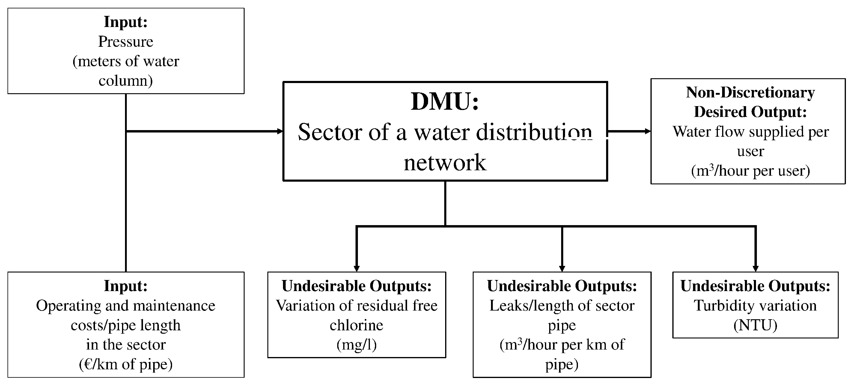
The selection of inputs, desired outputs, and undesirable outputs is always a challenge, depending on existing literature, the analyst’s criteria, and data availability. In the present case, the last factor mentioned was decisive in the selection of the two inputs, one desired output, and three undesirable outputs used (see Figure 1). This is because the study is strictly based on the variables provided by the company EMIVASA.

In spite of this, the variables used find support in the efficiency evaluation studies within the framework of the efficiency of the water distribution network: operating and maintenance costs [2,3,4,5,6,8,13,23,24,25,37,42], water flow supplied (water quantity) [3,4,5,6,8,23,25], leaks [3,14,26,42], pipe length of the sector [2,6,7,8,13,14,26,42], and number of users in the sector [4,6,8,13,25]. Like other studies in the literature [37], variables related to quality that have also been used in the literature on water distribution quality and health, are included: turbidity variation [75,76,77,78,79,80,81], variation of residual free chlorine [79,82,83,84,85,86,87,88,89], and pressure [90,91,92,93].

Regarding the chosen variables, it should be noted that:

• Sectors were divided by the length of the pipes in the sector to work with the unit value, since there were many differences in size between the sectors in operation and maintenance costs.
• The flow (defined as “delivered water flow divided by number of users”) was not considered a discretional or controllable output, but as a non-discretionary (or exogenously fixed) desired output; that is, managers cannot modify its level given that the demand that users require must be supplied.

The variables, constructed in this way, allow all sectors to be compared regardless of their size.

The water quality variables (provided by the company) indicate how these quality parameters change from the exit of the drinking water treatment plant to the DMU. In this context, they represent a loss of quality and have a negative impact on public health, which is why they are considered an undesirable output.

Table 1. Descriptive statistics for the variables (from Oct-2015 to Sep-2016).

	Inputs				Desired Outputs
	Pressure		Operating and Maintenance Costs/Pipe Length of the Sector		Flow Supplied/Users
Quarter	(Meters of Water Column)		(€/km Pipe)		(m3/Hour per Users)
	Mean	SD	Mean	SD	Mean	SD
2015 4th	104,024	17,148	413,271	468,980	0.142	0.470
2016 1st	105,278	23,592	446,036	449,470	0.143	0.462
2016 2nd	102,278	13,359	489,726	597,668	0.136	0.416
2016 3rd	99,715	12,356	548,224	923,062	0.128	0.364
Undesirable Outputs
	Leaks/Pipe Length of Sector		Turbidity Variation		Variation of Residual Free Chlorine
Quarter	(m3/Hour Per km Pipe)		(NTU)		(mg/L)
	Mean	SD	Mean	SD	Mean	SD
2015 4th	2921	1641	1272	0.860	1302	0.486
2016 1st	2919	1706	0.783	0.336	1229	0.555
2016 2nd	2865	1398	0.401	0.273	1328	0.407
2016 3rd	3070	0.364	0.329	0.280	1340	0.383

provides the descriptive statistics for the variables. Spearman’s correlation coefficient was used to ensure that there was no correlation between these variables within each analysis period.

Finally, mention should be made that the number of DMUs limits the number of variables that can be used in the analysis. This limitation was determined by Cooper’s rule, which is defined as $n\ge max\left\{m\times s,3\times \left(m+s\right)\right\}$, where n is the number of DMUs, m is the number of inputs, and s is the number of outputs [99]. Therefore, with a sample of 29 DMUs, this study obeyed Cooper’s rule because $29\ge max\left\{2\times 4,3\times \left(2+4\right)\right\}$, this is, $29\ge max\left\{4,18\right\}$.

In addition, given that EMIVASA provided data on the number of users, the length (in kilometres) of the pipelines in each sector, and kilometres of pipelines reviewed, for each of the sectors studied (DMUs) (see Appendix A

Table A2. Description of the sectors that use environmental variables.

DMU	Number of Users	Pipe Sector Length (Km)	Density (Users/Pipe Sector Length)	Revised Pipeline (Km)
1	9979	21,386	466.613672	25.6632
2	30,244	50.448	599.508405	60.5376
3	92	3.56	25.8426966	2.848
4	6695	30.397	220.251999	24.3176
5	577	2.151	268.247327	2.5812
6	16	3.103	5.15630035	2.4824
7	13,886	49.544	280.276118	59.4528
8	4482	14.248	314.570466	17.0976
9	2328	3.642	639.209226	4.3704
10	3778	14.675	257.444634	17.61
11	909	3.412	266.412661	2.7296
12	4216	18.249	231.026358	21.8988
13	488	4.401	110.88389	5.2812
14	196	2.355	83.2271762	1.884
15	2875	22.586	127.291242	18.0688
16	497	7.077	70.2274975	5.6616
17	2474	55.15	44.8594742	44.12
18	3149	16.206	194.310749	12.9648
19	5023	7.246	693.210047	8.6952
20	10,572	25.153	420.307717	30.1836
21	8536	25.819	330.609241	30.9828
22	553	6.396	86.4602877	5.1168
23	3529	23.393	150.857094	28.0716
24	11,441	18.833	607.497478	15.0664
25	3171	22.82	138.957055	18.256
26	1773	10.504	168.792841	8.4032
27	6429	10.994	584.773513	13.1928
28	21,616	39.575	546.203411	47.49
29	2684	6.11	439.279869	7.332

Source: EMIVASA.

), this makes it possible to carry out a second-stage analysis based on ANOVA.

5. Results for Case Study

The DEA–WRDD model presented in Section 3 was applied to the geographical area of the study, the city of Valencia, using the variables described in Section 4, to obtain the efficiency of each sector (DMU) of the water distribution network.

Table 2. Results of overall efficiency.

DMU	4th Quarter	1st Quarter	2nd Quarter	3rd Quarter
	2015	2016	2016	2016
1	0.387	0	0	0.397
2	0.213	0.092	0.199	0.414
3	0	0	0	0
4	0	0	0	0
5	0.482	0.325	0	0.473
6	0	0	0	0
7	0.262	0	0.347	0.44
8	0.237	0	0.139	0.381
9	0.387	0.334	0.305	0.447
10	0.128	0.282	0	0.45
11	0.278	0	0.274	0
12	0.265	0.157	0.275	0.503
13	0.377	0	0.205	0.431
14	0	0	0	0
15	0	0	0	0.233
16	0.134	0	0	0
17	0	0	0	0
18	0.064	0	0	0.246
19	0.34	0.308	0.434	0
20	0.218	0	0.167	0.424
21	0.468	0.344	0	0.281
22	0	0	0	0.076
23	0.356	0.26	0.373	0.455
24	0.373	0	0.226	0
25	0.16	0	0	0.292
26	0	0	0	0
27	0.205	0.054	0	0.387
28	0.303	0.156	0.324	0.473
29	0.22	0.148	0	0.336
Mean	0.202	0.085	0.113	0.246
SD	0.158	0.127	0.147	0.201

shows the overall efficiency of the 29 sectors. A value of 0 indicates that the sector is efficient. The further this value is from 0, the larger the inefficiency is.

The network sectors that are efficient in all quarters account for 20%, whereas the sectors classified as inefficient in all quarters make up 17% (the rest, 63%, are classified as inefficient in at least one quarter). The efficiency is generally lower in the fourth and third quarters than in the second and third quarters. Furthermore, in the third quarter, the efficiency is lower than the initial efficiency.

Table 3. Efficient DMUs evolution in percentage.

	4th Quarter	1st Quarter	2nd Quarter	3rd Quarter	Annual Mean
	2015	2016	2016	2016
Efficient Sectors (%)	0.28	0.59	0.59	0.31	0.44
Mean	0.2	0.08	0.11	0.25	0.16
SD	0.16	0.13	0.15	0.2	0.16

shows the percentages of efficient sectors per quarter, the mean values, the standard deviation per quarter, and the annual mean value. On average, the percentage of efficient network sectors is 44%. The quarters with the highest percentage of efficient sectors are the first and second quarters. Thus, the average value of inefficiency falls into the first quarter before increasing. This increase is particularly notable from the second to the third quarter.

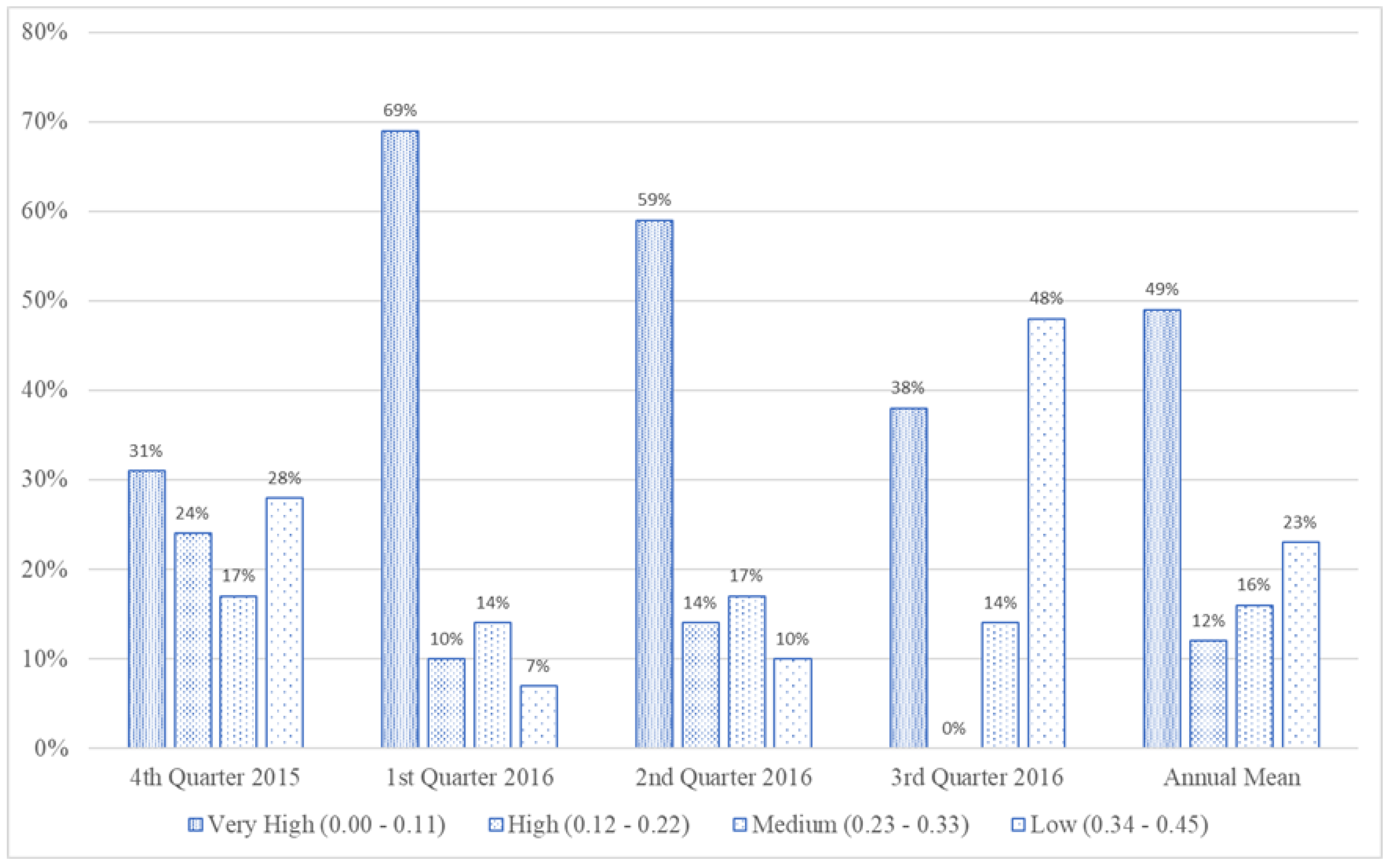
Figure 2 shows the percentage of efficient sectors in each quarter in terms of four efficiency levels from very high to low. The average annual value is also to check the change in the efficiency level of each sector over time. On average over the year, 49% of the network sectors have very high efficiency.

With regard to change in efficiency over time, efficiency (irrespective of the category) improves in the first quarter, declines slightly in the second quarter, and then declines sharply in the third quarter. The medium category (0.23–0.33) is more stable over time than the other categories. Notably, there is a large decrease in efficiency in the second quarter, explained by the large increase in the low efficiency category, coupled with the decrease and absence of sectors in the very high and high categories, respectively.

Once the efficiency indices have been obtained, the objective is to evaluate the possible relationships between these measures and some explanatory variable. To do this, a second-stage analysis was applied to the results obtained using the DEA–WRDD model and to two characterizing variables of urban water distribution networks, namely the density (understood as the number of users per kilometer of pipes) and the kilometers of pipeline revised (specifically, the percentage of the pipelines of the network that during the study period (annual) were reviewed to check the level of leaks in the sector). Among the options offered by the literature, a one-way analysis of variance (ANOVA) was considered appropriate.

The analysis of variance tries to identify if there are significant differences between the mean values of the variables “density” and “kilometres of pipes reviewed” as a function of the efficiency indices obtained. In the

Table 4. Analysis of Variance ANOVA: KMs revised pipes.

Groups	N	Sum	Mean	Variance
Annual average efficiency	29	4.68	0.1614	0.0149
% KMs revised pipes	29	28.40	0.9793	0.0410
Sources of Variations	Sum Sq	Df	Mean Sq	F-test	P-Level	Crit F-Value
Between groups	9.7006	1	9.7006	346.9311	0.0000	4.0130
Within groups	1.5658	56	0.0280
Total	11.2665	57

and

Table 5. Analysis of Variance ANOVA: Users/KMs of network.

Groups	N	Sum	Mean	Variance
Annual average efficiency	29	4.68	0.1614	0.0149
Users/KMs of network	29	8372	288.7002	42,318.4238
Sources of Variations	Sum Sq	Df	Mean Sq	F-Test	P-Level	Crit F-Value
Between groups	9.7006	1	9.7006	346.9312	0.0000	4.0130
Within groups	1,184,916	56	21,159.2194
Total	2,392,109	57

, we can see how, with 5% significance, the F statistic leads to rejecting the null hypothesis of equality of means between the two groups, and it can be accepted that the differences observed in the mean values for the reference indices of the different groups are not random.

As mentioned in Section 3, one of the main advantages of the DEA–WRDD model is that it gives an efficiency value for each variable.

Table A1. Efficiency of the variables by quarter.

DMU	Pressure		Operating and Maintenance Costs/Pipe Length of the Sector		Leaks/Pipe Length of the Sector		Turbidity Variation		Variation of Residual Free Chlorine
	(P)		(O&M)		(F)		(T)		(Cl)
1	0.268	0	0.685	0	0.316	0	0.233	0	0.345	0
	0	0.065	0	0.868	0	0.604	0	0.341	0	0.035
2	0.156	0	0.477	0.179	0	0.302	0.133	0.459	0.199	0.166
	0.086	0.11	0.179	0.868	0.153	0.446	0	0.56	0	0.012
3	0	0	0	0	0	0	0	0	0	0
	0	0	0	0	0	0	0	0	0	0
4	0	0	0	0	0	0	0	0	0	0
	0	0	0	0	0	0	0	0	0	0
5	0.204	0	0.933	0	0.484	0	0.176	0	0.529	0
	0.081	0	0.733	0.956	0.692	0.781	0	0.541	0.036	0.08
6	0	0	0	0	0	0	0	0	0	0
	0	0	0	0	0	0	0	0	0	0
7	0.256	0.087	0.304	0.513	0.274	0.627	0.16	0.554	0.297	0
	0	0.034	0	0.804	0	0.38	0	0.645	0	0.357
8	0.205	0	0.532	0.247	0	0.079	0.234	0.381	0.081	0
	0	0.07	0	0.719	0	0	0	0.897	0	0.205
9	0.286	0	0.686	0.507	0.49	0.363	0.251	0.54	0.126	0.165
	0	0.079	0.72	0.785	0.42	0.27	0.374	0.893	0.132	0.222
10	0	0	0.513	0	0	0	0	0	0	0
	0.055	0.121	0.697	0.443	0.561	0.654	0	0.905	0	0.292
11	0.288	0.337	0.583	0.453	0.048	0.152	0	0.044	0.316	0.262
	0	0	0	0	0	0	0	0	0	0
12	0.206	0.15	0.516	0.557	0	0.456	0.127	0.05	0.379	0.084
	0.141	0.074	0	0.748	0.364	0.675	0.151	0.919	0.217	0.191
13	0.231	0.021	0.598	0.215	0.082	0.305	0.256	0.372	0.681	0.197
	0	0.02	0	0.518	0	0.773	0	0.716	0	0.292
14	0	0	0	0	0	0	0	0	0	0
	0	0	0	0	0	0	0	0	0	0
15	0	0	0	0	0	0	0	0	0	0
	0	0	0	0.219	0	0.252	0	0.364	0	0.452
16	0	0	0.369	0	0.022	0	0.227	0	0	0
	0	0	0	0	0	0	0	0	0	0
17	0	0	0	0	0	0	0	0	0	0
	0	0	0	0	0	0	0	0	0	0
18	0	0	0.079	0	0	0	0.025	0	0.238	0
	0	0	0	0	0	0.244	0	0.834	0	0.397
19	0.352	0.207	0.358	0.704	0.258	0.681	0.222	0.555	0.494	0
	0.057	0	0.797	0	0.191	0	0.185	0	0.19	0
20	0.316	0	0.274	0.192	0.1	0.155	0.169	0.247	0.157	0.311
	0	0.178	0	0.735	0	0.322	0	0.561	0	0.29
21	0.209	0	0.86	0	0.425	0	0.145	0	0.633	0
	0	0	0.772	0.288	0.778	0.76	0.096	0.214	0.032	0.283
22	0	0	0	0	0	0	0	0	0	0
	0	0	0	0	0	0	0	0.41	0	0.045
23	0.172	0.134	0.625	0.592	0	0.505	0.423	0.443	0.516	0.199
	0.071	0.095	0.315	0.811	0.552	0.063	0.18	0.9	0.248	0.406
24	0.328	0	0.735	0.451	0.328	0.052	0.147	0.371	0.165	0.259
	0	0	0	0	0	0	0	0	0	0
25	0	0	0.409	0	0.178	0	0.171	0	0	0
	0	0	0	0.491	0	0.121	0	0.568	0	0.325
26	0	0	0	0	0	0	0	0	0	0
	0	0	0	0	0	0	0	0	0	0
27	0.295	0	0.122	0	0.098	0	0.188	0	0.319	0
	0.004	0.071	0.044	0.626	0.252	0.329	0	0.72	0	0.224
28	0.295	0	0.304	0.416	0.317	0.539	0.19	0.444	0.409	0.34
	0	0.062	0.072	0.833	0.415	0.541	0.094	0.726	0.319	0.228
29	0.319	0	0.08	0	0.278	0	0.064	0	0.377	0
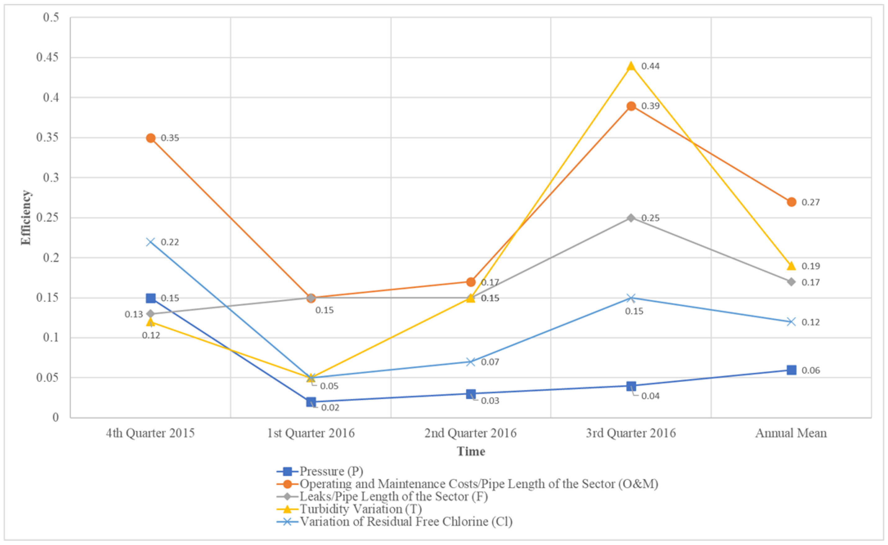
	0.011	0.143	0.131	0.549	0.107	0.045	0.24	0.909	0.33	0.022

in the Appendix shows the efficiency of each variable by quarter. The desired output “Flow supplied per user” is not included because it is a non-discretionary variable (managers cannot modify its level because it is determined by user’s demand). To interpret the results, the criteria explained above (for Table 2) are followed: a value equal to 0 indicates that the variable is efficient, while the further it is from 0, the greater the inefficiency is. To show the efficiency of each variable, the mean values by quarter are summarized in Figure 3.

The annual efficiency values for the inputs show that the pressure variable (P) is more efficient than the operating and maintenance costs per length of pipe in the sector (O&M) variable. However, the values of P reflect a decrease in the mean value of quarterly efficiency. For the O&M variable, the average value of efficiency improves in the first quarter and subsequently decreases in the second quarter and, especially, the third quarter.

The undesirable outputs have similar annual mean values. Variable F shows an improvement in efficiency in the first quarter, which remains constant in the second quarter and then decreases in the third quarter. The variables F and Cl improve in terms of efficiency in the first quarter, then decrease in the second and third quarters. This decrease in efficiency is more pronounced for variable T than for the other variables.

6. Discussion

The results shown in Table 2 provide evidence that the sectors’ efficiency decreases in the second and third quarters (after an increment in the first quarter). Furthermore, the analysis of efficiency by variables reveals the same pattern as that observed for general efficiency. A possible explanation of this trend in the value of inefficiency could be the presence of seasonality in water consumption (in the city of Valencia, in summer, water consumption is reduced by between 5% and 10% compared to the annual average [1]) or the temperature in these quarters (the higher the temperature, the more pipe breaks that increase leakage, which in turn leads to an increase in turbidity and a decrease in free chlorine residual [100,101,102,103]).

Although these aspects are not considered in this paper, a possible explanation for the efficiency results obtained is the possible relationship between temperature and efficiency. Starting from the initial state of the fourth quarter of 2015 (from October to December), the efficiency reaches its maximum in the winter months (first and second quarters of 2016, from January to March) to later decrease in the following two quarters as the temperature increases. The justification is that the higher the temperature, the greater the risk of leaks and a possibly greater turbidity variation and more residual free chlorine decrease.

It may be relevant to note that the first and second quarters show the same percentage of efficient sectors, but the average value of efficiency decreases (see Table 3), which already represents a slight trend that may indicate the aforementioned possible relationship between efficiency and temperature.

Regarding the second-stage analysis, the ANOVA analysis (see Table 4 and Table 5) points to the existence of a link between higher efficiency and, on the one hand, revised kilometres of pipes and, on the other, users per kilometre of pipes (density): the corresponding average efficiency index of the sectors with a higher percentage of revised pipe kilometres and the sectors with a higher density are clearly shown, always on average, above the sectors with a lower percentage of revised pipe kilometres or with lower density. Since pipe density is related to population density, the relationship noted should not be surprising since population density, as a factor that defines one of the particular characteristics of the surroundings, has a statistically significant impact on the indexes of efficiency [34].

These results make it possible to verify the influence of these factors on the efficiency indicators obtained through DEA-WRDD.

Concerning inputs, the results of the efficiency analysis applied to the variables indicate that not all of them are used efficiently. The efficiency values for the inputs show that the pressure variable (P) is used more efficiently than O&M variable. This greater efficiency may be because, in comparative terms, the P input remains more constant than the O&M input since it is a “service variable” that is regulated and that must meet the established value to guarantee users a certain water pressure level [104]. The O&M input depends on other factors such as age, useful life, material, temperature, and so on. Therefore, it experiences some variations.

The undesirable outputs (F, T, and Cl) have similar annual mean values, and the variation in residual free chlorine and leaks per length of sector pipe generate fewer inefficiencies than turbidity variation. This similarity is because, according to the principles of hydraulics, they are “service variables” that are closely related to each other. Variable F, which has the highest annual inefficiency, affects turbidity variation directly and proportionally and the level of chlorine inversely [104,105].

Therefore, in order to improve the overall efficiency of each sector, it is necessary to act on the variables or sets of variables with the highest inefficiency values. On one hand, in general, implementing measures that reduce O&M costs will improve efficiency more than implementing measures that improve pressure. On the other hand, given that the average values of the undesired outputs are similar, acting on any of them will generate an increase in overall efficiency. However, it would be necessary to analyze the results of each sector in order to make the best decision to improve the efficiency of that sector.

All in all, this study has certain limitations related to the data. One is that available data only refer to one year, and it is impossible to verify the existence of seasonality. Another is the number of variables used, as we consider using only five variables to be weak and insufficient, but these variables are the ones that the company decided to provide us with. On the other hand, given that the objective of this work is basically to transfer a methodology for the management of sectorized water distribution networks, the companies that apply it in the future will have and will be able to use more variables for periods and stakeholder and sectors of interest.

7. Conclusions

The sectorization of hydraulic networks, among other advantages, allows a better and earlier detection of possible anomalies in the networks and allows limiting the operating range in case of repairs and maintenance work, thus minimizing the inconvenience to neighbor if work is needed. In addition, sectorizing the water network allows maintaining continuous control of the flows that run through each area, avoiding unnecessary water losses and consumption and achieving significant savings in drinking water. Thus, with sectorization, it is possible to improve hydraulic performance and control over parameters that affect water quality.

However, we are not aware that the literature has addressed the issue of sectorization efficiency, despite being of great importance to optimize the use of a scarce resources such as water for urban use. This lack of studies is more noticeable regarding the efficiency of the networks that have already been sectorized.

On this basis, the aim (and novelty) of this work is to provide a methodology to analyze the efficiency of networks by focusing on individual sectors (DMUs are considered each sector of the city’s distribution network as an independent unit of analysis) and applying the data-envelopment-analysis weighted-Russell-directional-distance (DEA-WRDD) model.

Unlike the previous models (which have the limitation of that they cannot provide individual (in)efficiency scores by variables), the advanced model WRDD addresses all these issues to make better management decisions. In this way, the main advantage of the model is that it combines Directional Distance Function (DDF) along with a non-radial model used in the evaluation of each variable contribution to inefficiency component. This makes it possible to understand its impact on changes in the efficiency of the decision-making units.

The application of the DEA–WRDDM model to sectorized water distribution networks may allow optimizing resources when it comes to improving management and efficiency. In the first place, knowing the comparative efficiency of each sector of the water distribution network allows deciding which sectors to act on to improve efficiency as a priority. Second, the WRDDM shows the efficiency of each variable. With this information, it is possible to know which variables or sets of variables determined the overall efficiency. Then, managers may use this information to improve efficiency and optimize the water distribution sector.

The city of Valencia was chosen as the study area. Valencia’s distribution network has 47 sectors and serves a population of almost 800,000 inhabitants. Based on the data provided by EMIVASA and a review of the literature, two inputs (pressure and operating and maintenance costs by length of pipe in the sector), one desired output (flow supplied/users), and three undesirable outputs (leaks/pipe length of the sector, turbidity variation, and variation in residual free chlorine) were chosen (obviously, in a future application, the water supply management companies may use different variables depending on their business objectives).

In the particular case analyzed, the results of the DEA–WRDDM analysis point to the existence of a seasonality factor in efficiency and show that almost half of the sectors analyzed have a very high efficiency, although the results of the analysis applied to each of the variables indicate that not all of these are used efficiently.

This methodology can be useful for water utilities. The specific results obtained by applying the DEA–WRDD model can allow managers to detect in which sectors of the water distribution network and in which specific variables they need to act in order to improve the efficiency of the service.

Information on the efficiency level of each network sector may allow managers to objectively determine which sectors should be prioritized over others when making investments and improvements. Furthermore, as the DEA–WRDD model gives the efficiency of each analyzed variable. Moreover, as the DEA–WRDD model provides the (in)efficiency of each variable analyzed and the (in)efficiency of each variable in each sector, it may be possible to detect which variable results in a lower level of efficiency. By doing so, specific measures or actions can be taken to improve the efficiency of variable, of the sector, and of the network.

Finally, as future lines of research, if the company provided us with a longer time series, we would study the existence (or not) of seasonality of efficiency. Likewise, with temporal data of the sectors, we could apply a panel data model to estimate the variables on which the efficiency of water distribution network sectors depends (age or materials of the pipes, percentage of revised pipes, density understood as users per km of pipes, investments made in the sector, seasonality in water consumption, temperature, etc.). Such research could provide a detailed explanation of the results presented here. Regardless of obtaining new data, with data used for this study, we propose carrying out an analysis of efficiency using a Fuzzy Data Envelopment Analysis (Fuzzy-DEA) to relax the assumption that flow is a non-discretionary and non-controlling factor.