
A Dragonfly Optimization Algorithm for Extracting Maximum Power of Grid-Interfaced PV Systems

 ,
,  , ,
, ,
Abstract
:1. Introduction
- The proficient and enhanced dragonfly optimization algorithm (DOA) was implemented.
- The suggested MPPT method can track the global MPP with fewer iterations under partial shading.
- The proposed DOA’s applicability was supported by the performance comparison with existing PSO, improved PSO, and P&O algorithm.
- The proposed DOA effectively applied to the PV-interfaced grid with the help of VSI that can efficiently transfer energy between the PV array and grid side.
2. Modeling of PV Array and Partial Shading
2.1. PV Array Modelling
2.2. Behavior of PV Array under Partial Shading
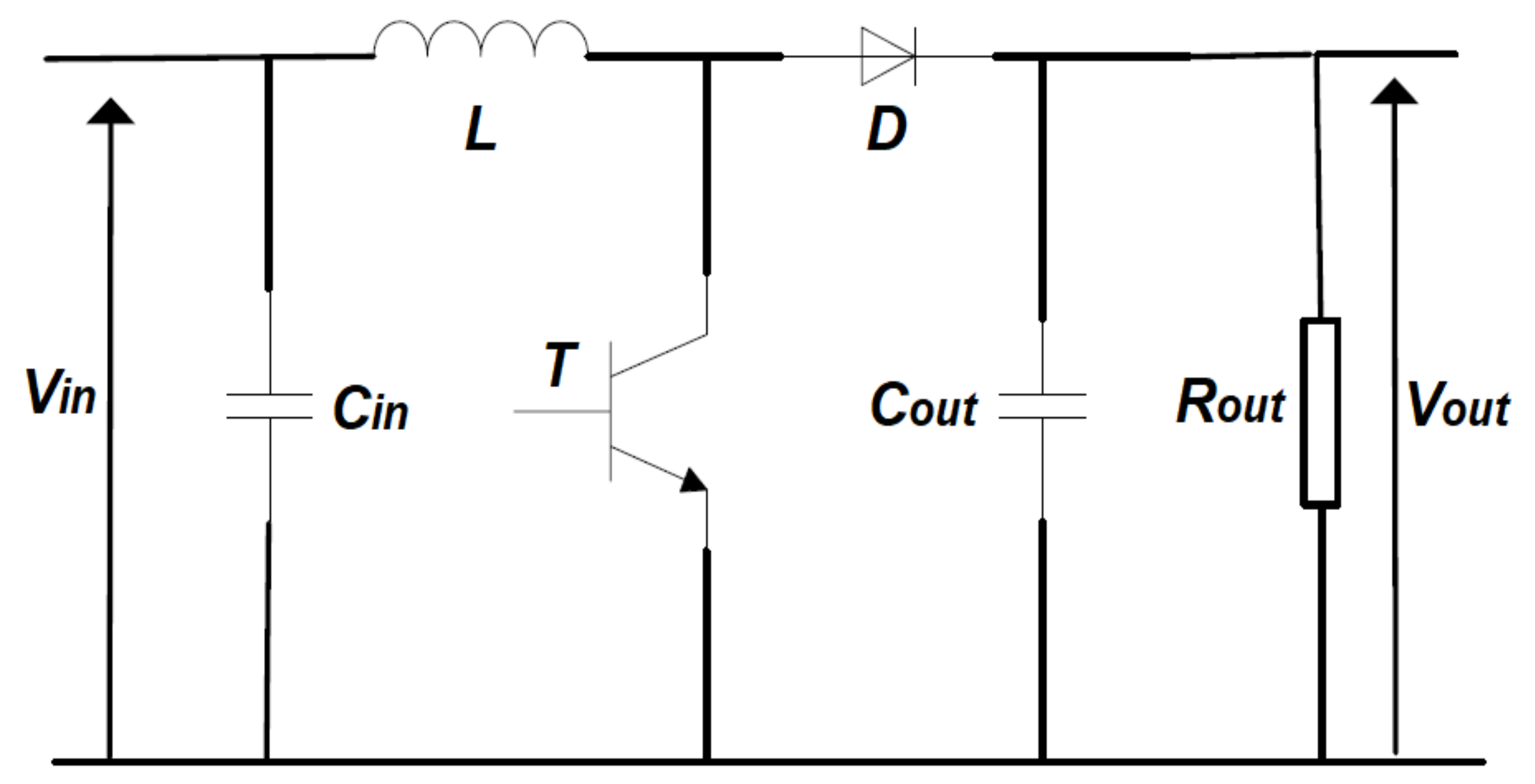
2.3. Boost Converter Modelling
3. MPPT Algorithms
3.1. Dragonfly Optimization Algorithm (DOA)
3.2. Application of DOA for MPPT Problem
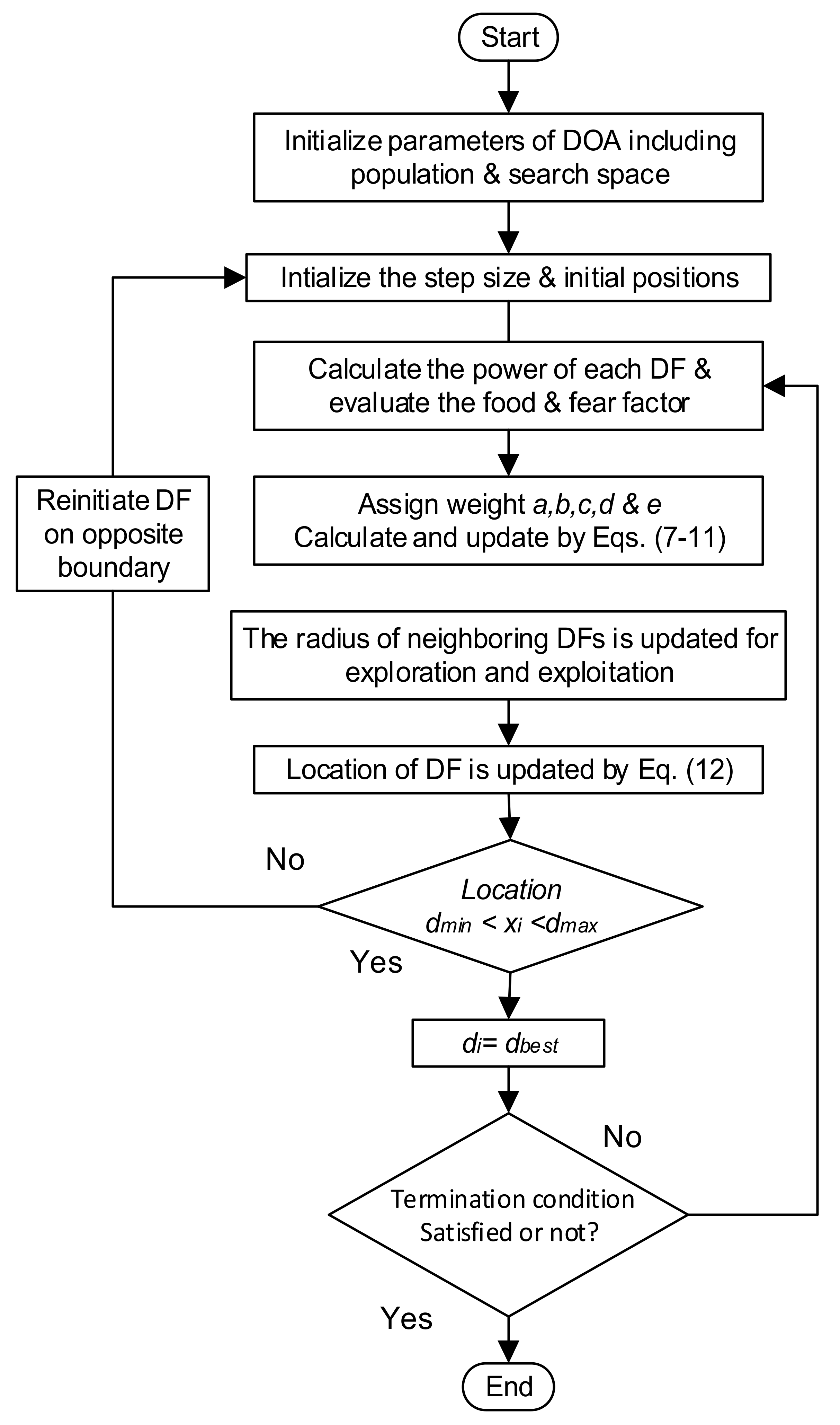
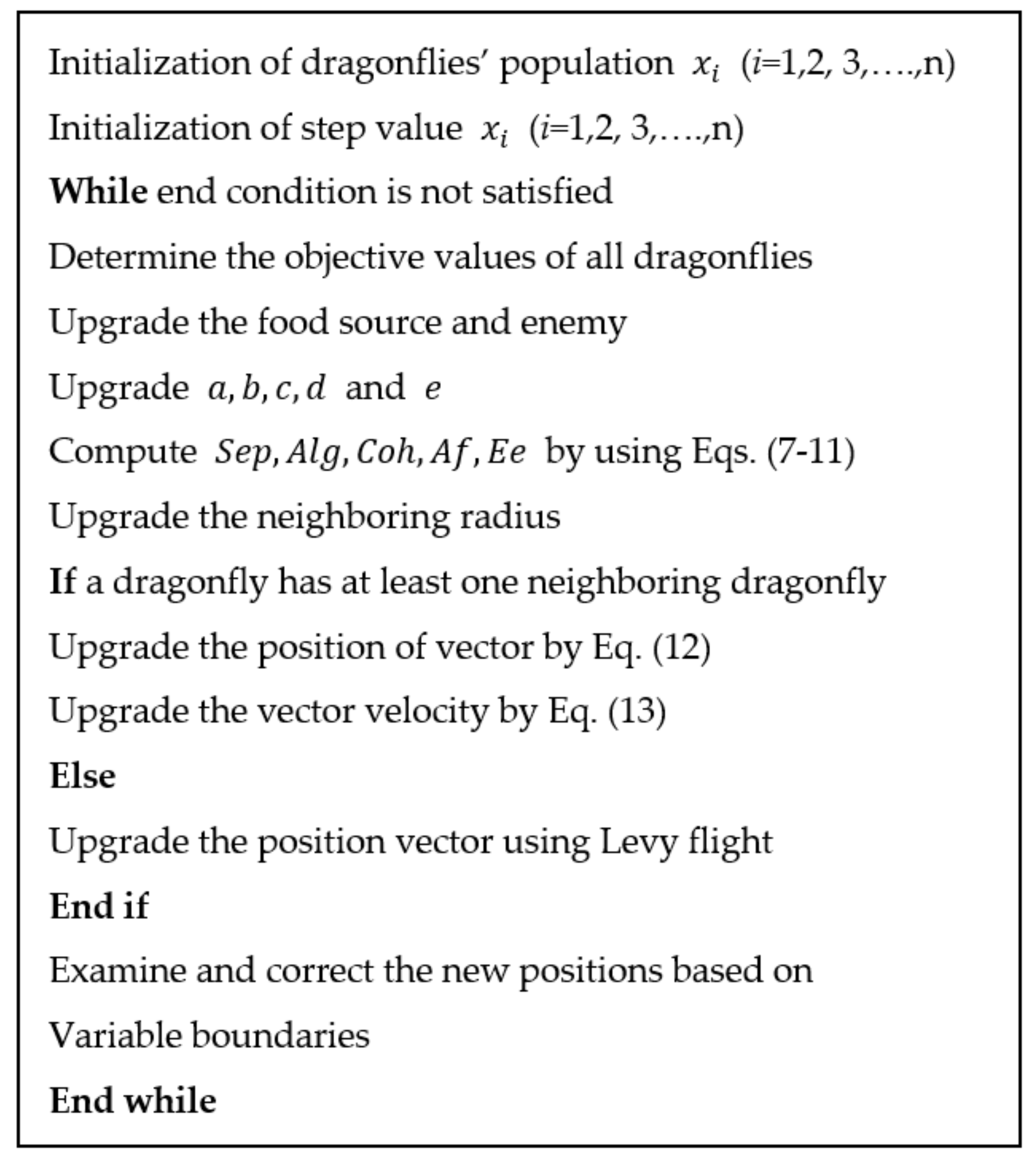
- Firstly, there is a need to initialize the particles around the search space between dmin and dmax, and the step value () for particles is initialized properly. The duty cycle is considered as the particle position and its value is randomly chosen between 0.2 and 0.9.
- During the second step, the boost converter is triggered by utilizing the control algorithm against each particle position and the best output power that is assumed to be the fitness (cost) function is calculated. Then, the food source and enemy location are updated. The cost function is monitored for changes and if there is any variation in power due to partial shading.
- Subsequently, the a, b, c, d, and e values are updated. The separation, alignment, cohesion, food, and enemy features for individual DFs are calculated by using Equations (7)–(11). For exploration and exploitation, the radius of neighboring dragonflies is updated.
- At this moment, the step and position of particle is calculated by using Equations (12) and (13) respectively. If the position of dragonflies lies outside the search space, then DOA is initiated at opposite boundary.
- Finally, if the termination condition (the best optimal position of dragonflies to operate on global MPP) is met or satisfied, then this algorithm will stop. It also restarts the search process if a sudden change occurs in the input power.
3.3. Comparison of DOA with Other MPPT Techniques
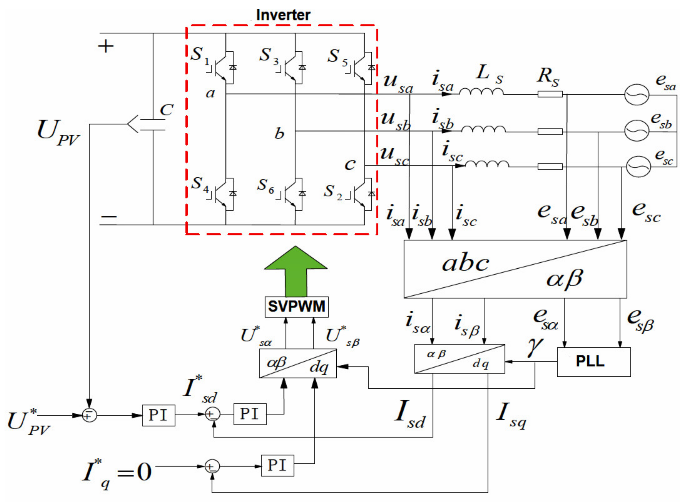
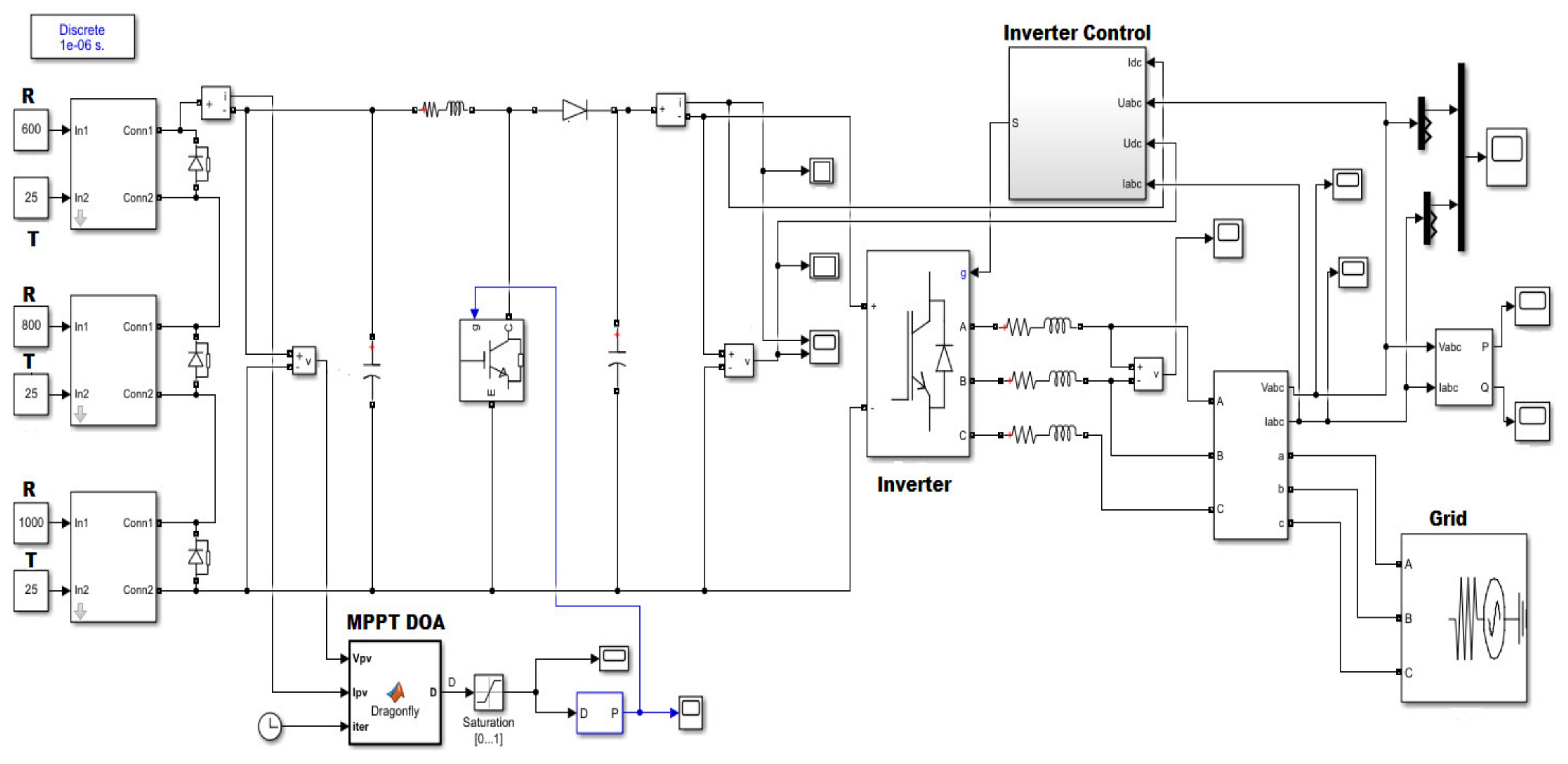
4. Inverter Control Methodology
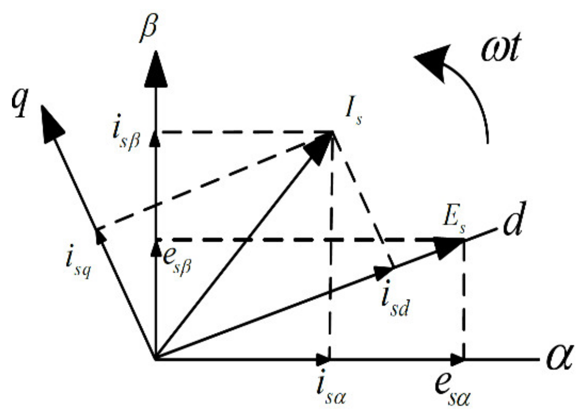
4.1. Voltage and Current Control Strategy
4.2. SVPWM Technology
4.3. Grid Connected Filter
5. Simulation Results and Discussion
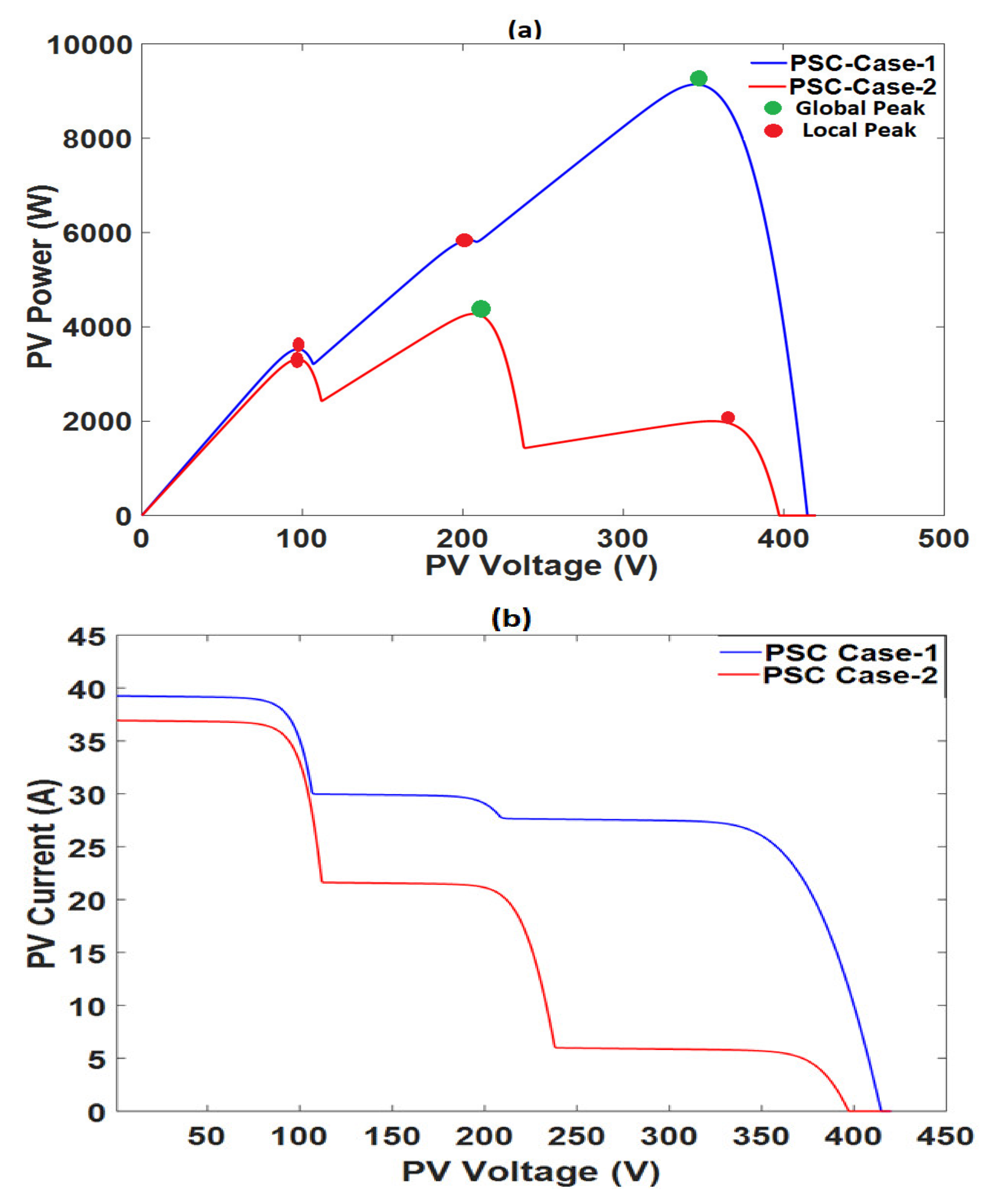
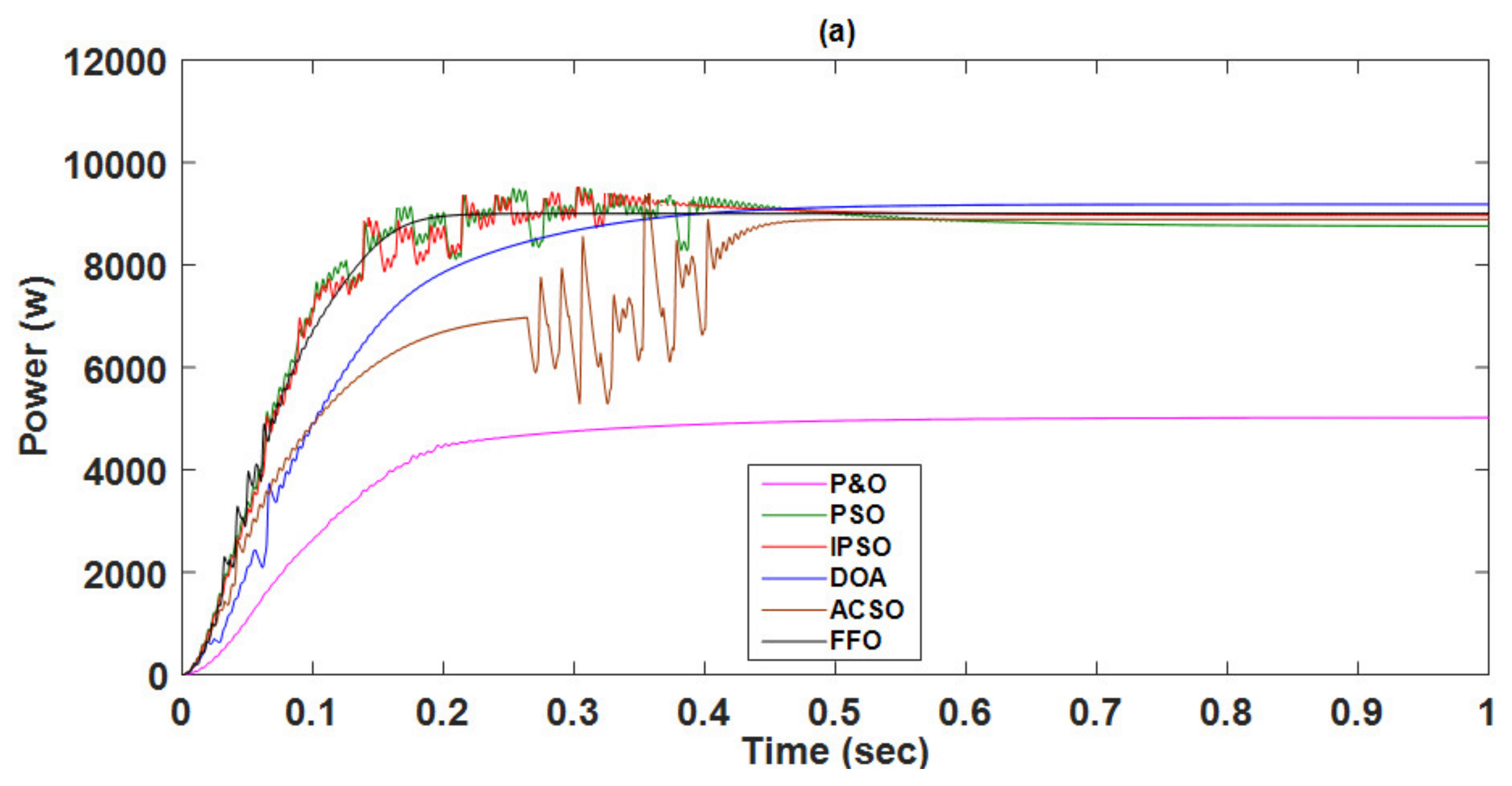
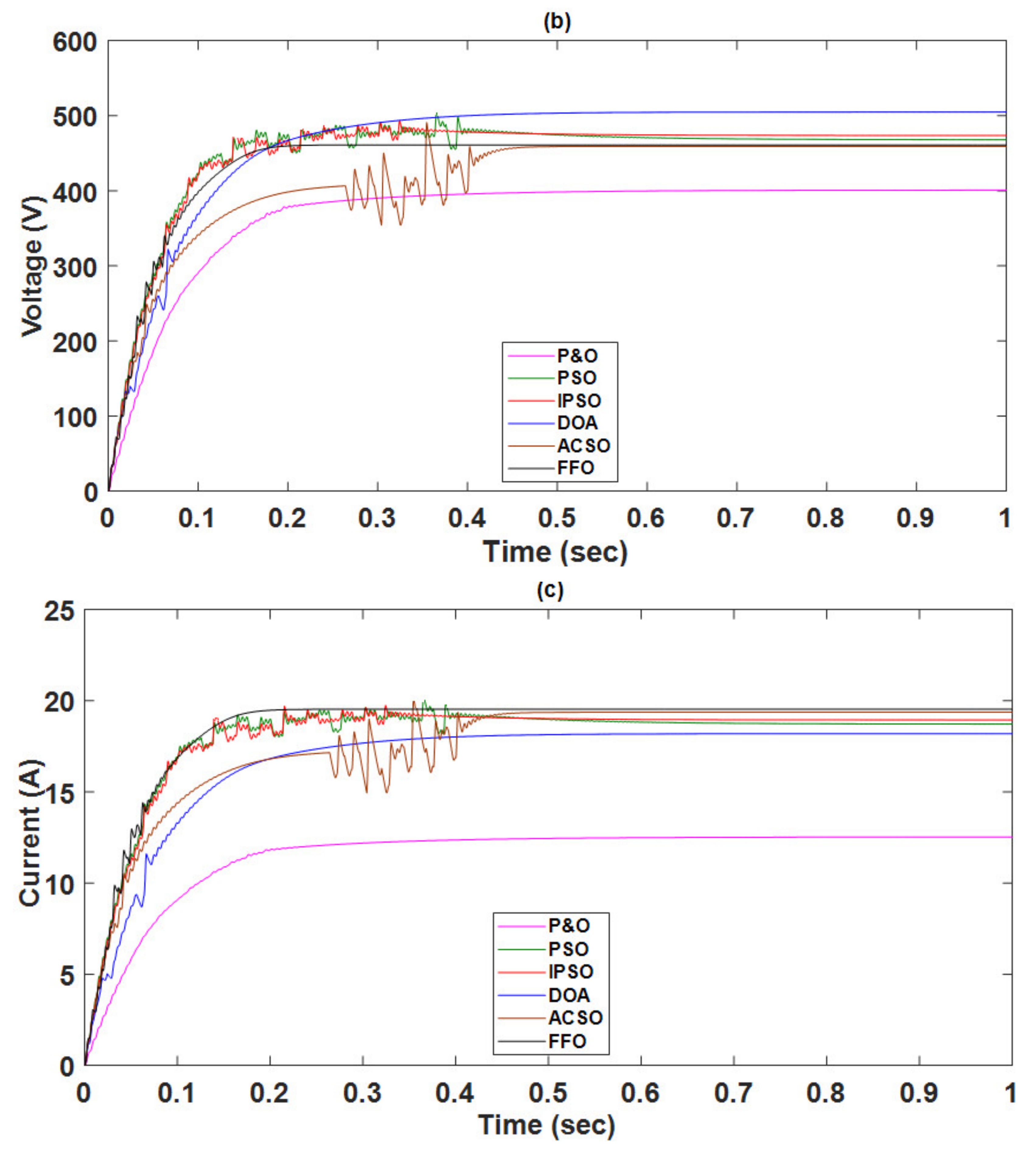
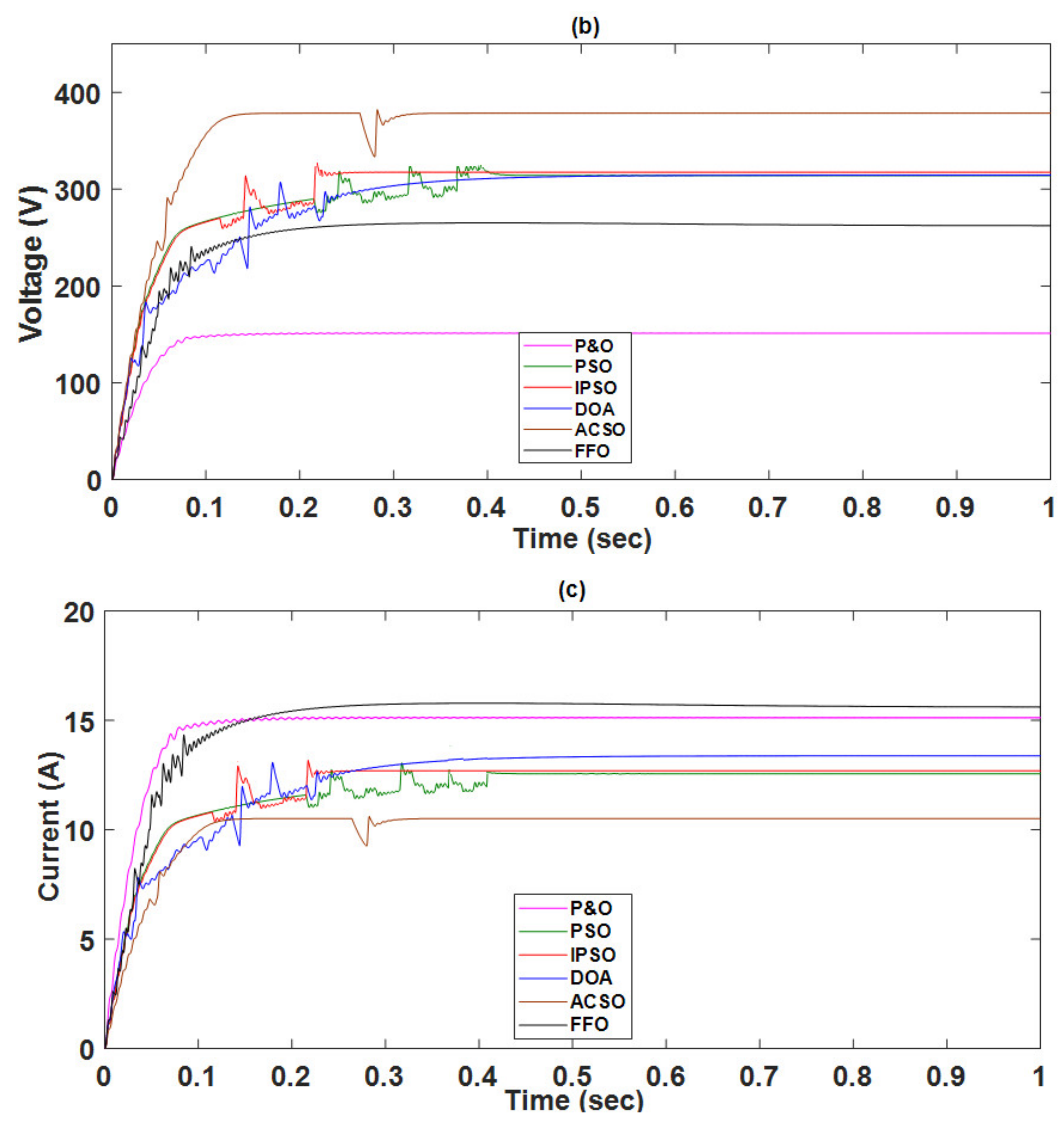
5.1. Partial Shading Case-1
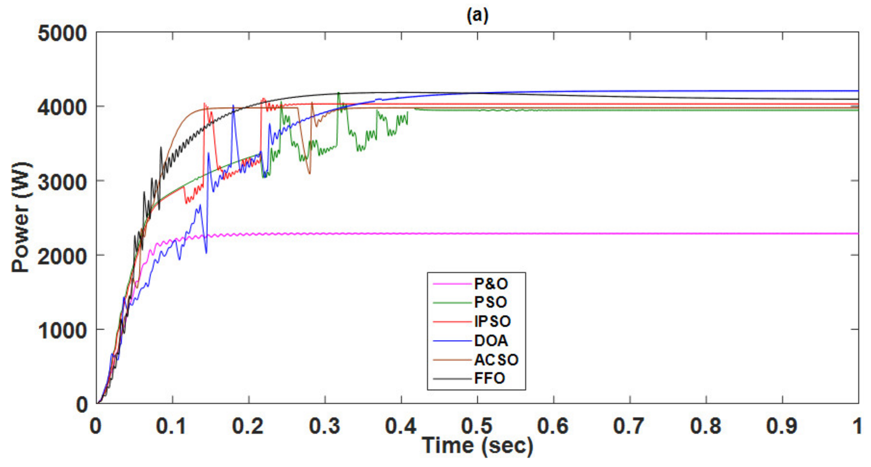
5.2. Partial Shading Case-2
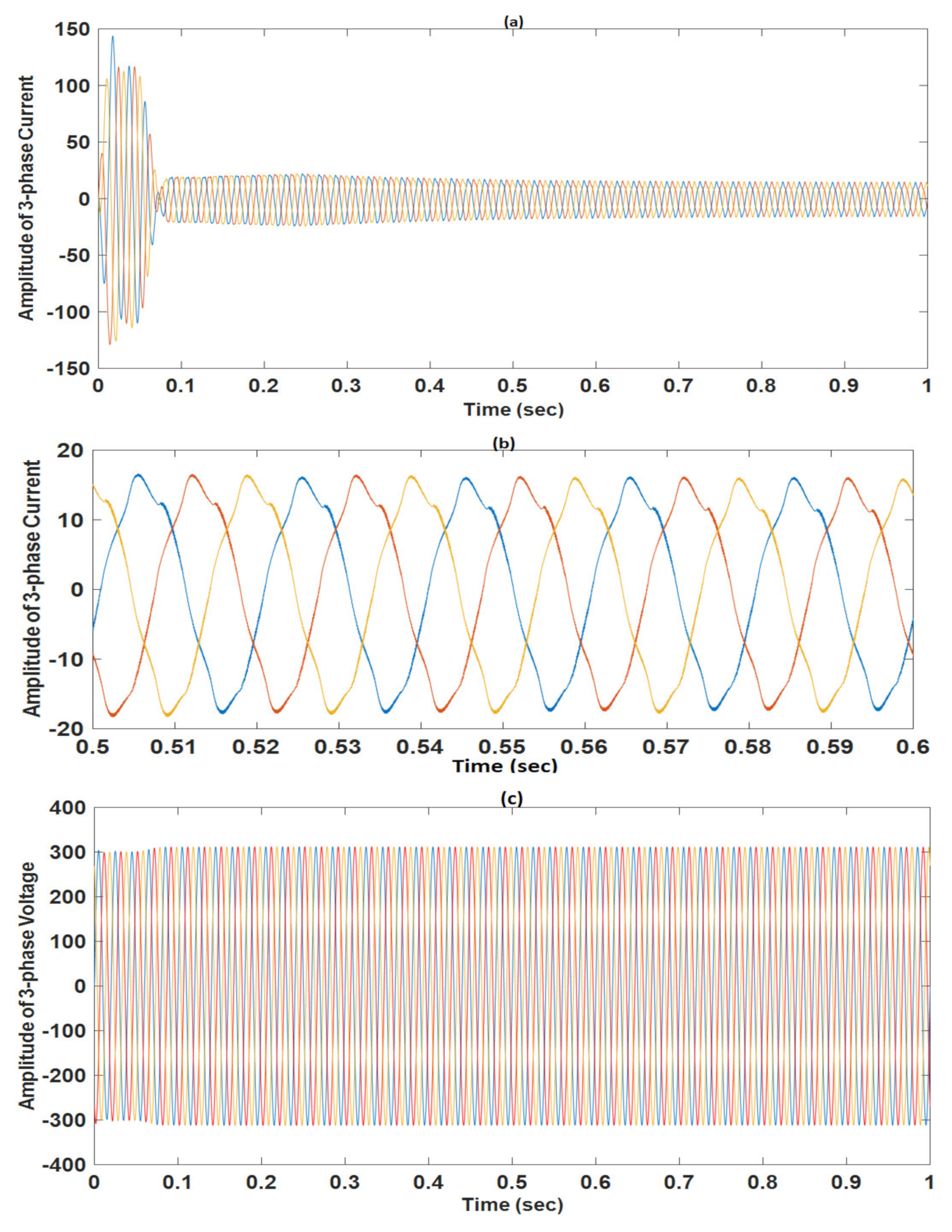
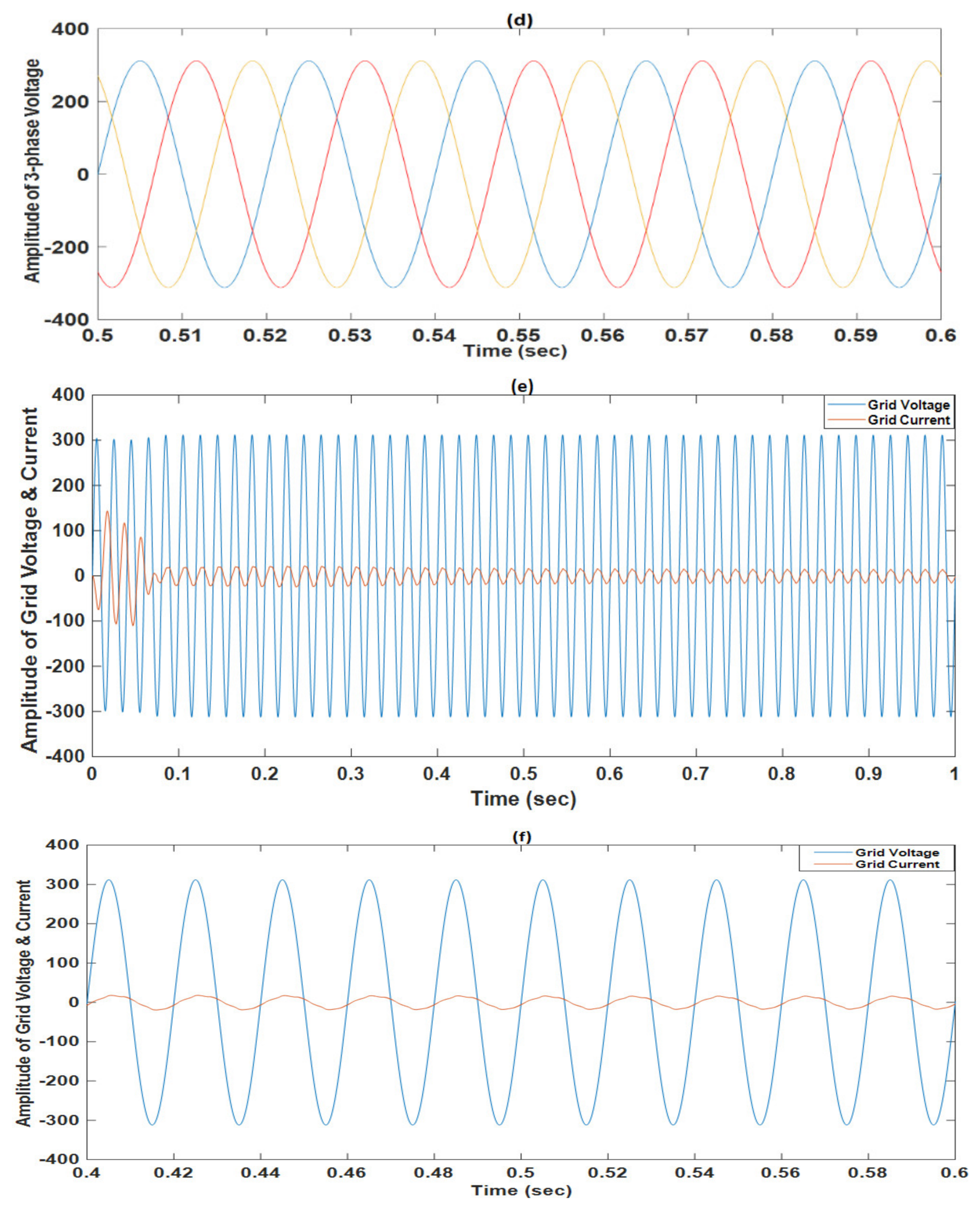
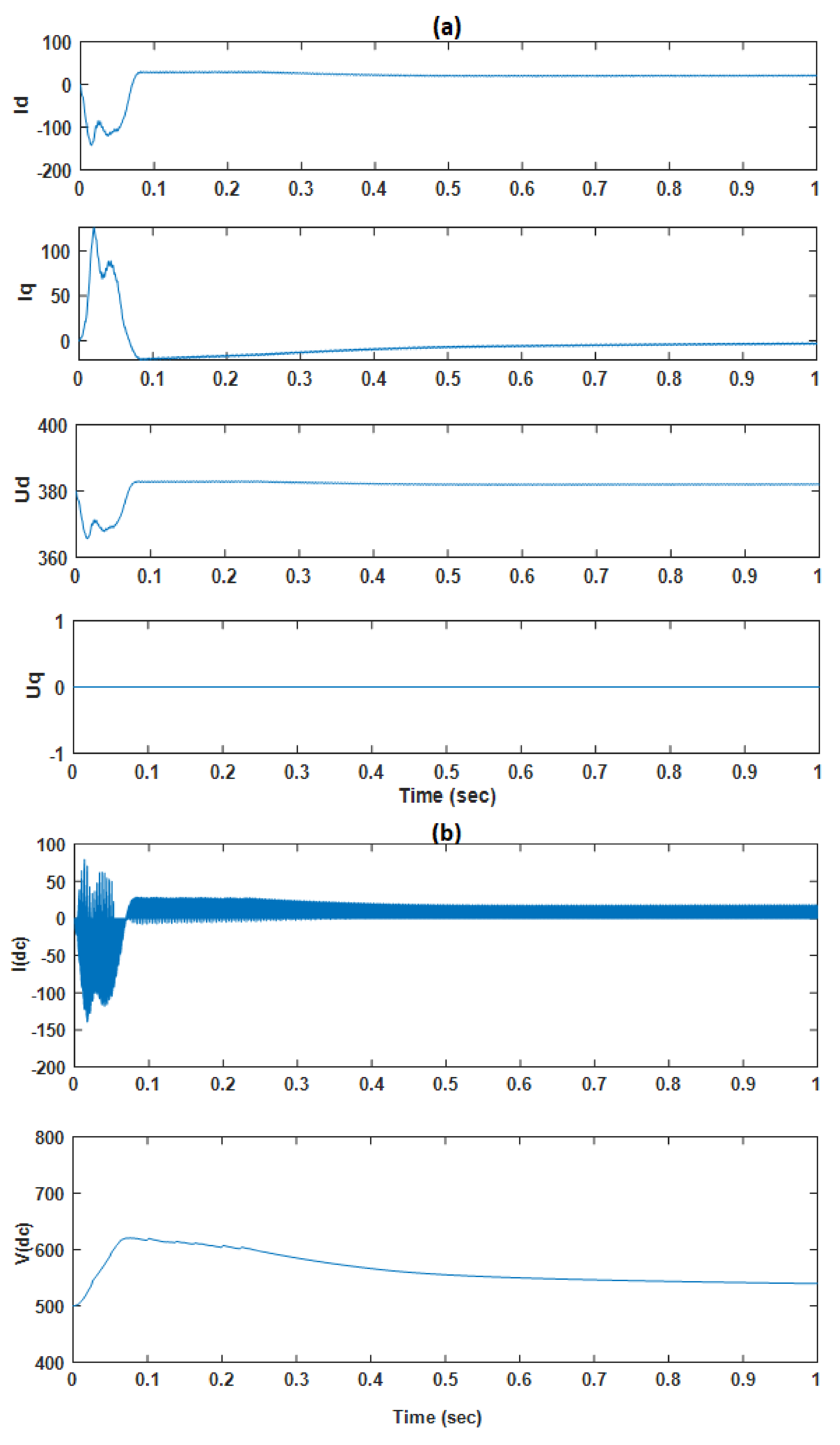
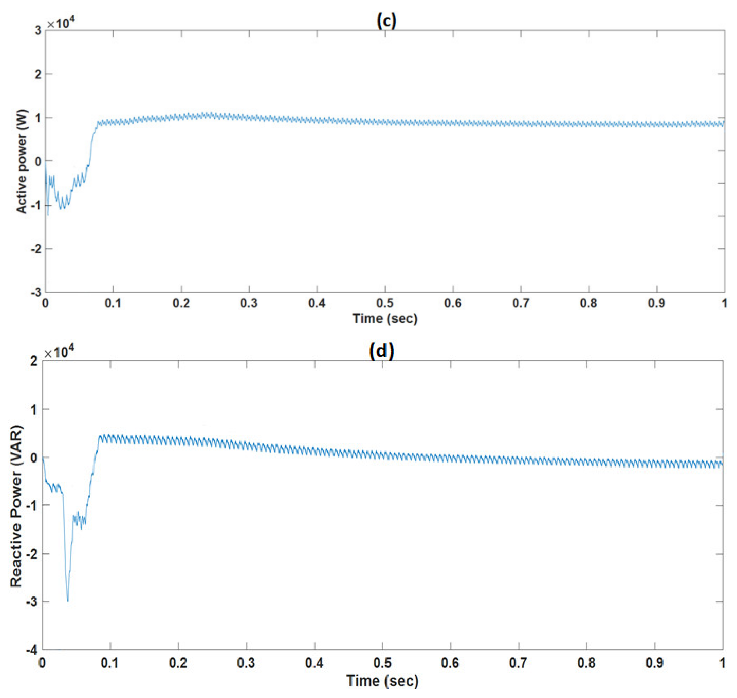
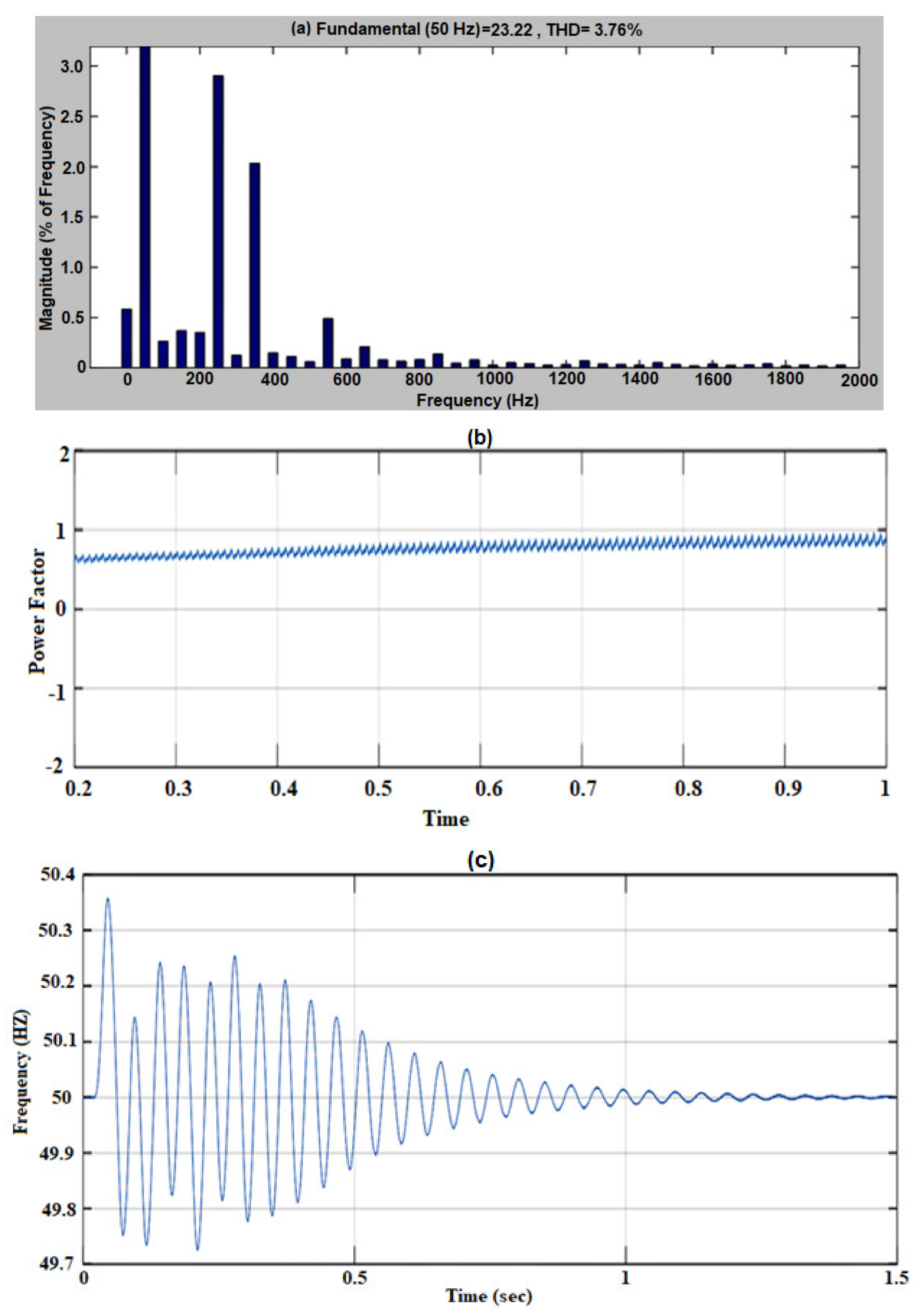
5.3. PV Array Interfaced with Grid Network
6. Conclusions
Author Contributions
Funding
Institutional Review Board Statement
Informed Consent Statement
Data Availability Statement
Conflicts of Interest
Appendix A

| Parameters | Values |
|---|---|
| Input Voltage | 337 V |
| Output Voltage | 540 V |
| PV maximum Power | 12,000 W |
| Frequency | 10 K Hz |
| Inductor ripple current | 10% |
References
- Li, K.; Liu, C.; Jiang, S.; Chen, Y. Review on hybrid geothermal and solar power systems. J. Clean. Prod. 2020, 250, 119481. [Google Scholar] [CrossRef]
- Agathokleous, R.A.; Kalogirou, S.A. Status, barriers and perspectives of building integrated photovoltaic systems. Energy 2020, 191, 116471. [Google Scholar] [CrossRef]
- Fathabadi, H. Novel stand-alone, completely autonomous and renewable energy based charging station for charging plug-in hybrid electric vehicles (PHEVs). Appl. Energy 2020, 260, 114194. [Google Scholar] [CrossRef]
- Vezin, T.; Meunier, S.; Quéval, L.; Cherni, J.; Vido, L.; Darga, A.; Dessante, P.; Kitanidis, P.; Marchand, C. Borehole water level model for photovoltaic water pumping systems. Appl. Energy 2020, 258, 114080. [Google Scholar] [CrossRef]
- Aziz, A.S.; Tajuddin, M.F.N.; Adzman, M.R.; Mohammed, M.F.; Ramli, M.A. Feasibility analysis of grid-connected and islanded operation of a solar PV microgrid system: A case study of Iraq. Energy 2020, 191, 116591. [Google Scholar] [CrossRef]
- Lodhi, E.; Jing, S.; Lodhi, Z.; Shafqat, R.N.; Ali, M. Rapid and Efficient MPPT Technique with Competency of High Accurate Power Tracking for PV System. In Proceedings of the 2017 4th International Conference on Information Science and Control Engineering (ICISCE), Changsha, China, 21–23 July 2017; pp. 1099–1103. [Google Scholar] [CrossRef]
- Ishaque, K.; Salam, Z. A review of maximum power point tracking techniques of PV system for uniform insolation and partial shading condition. Renew. Sustain. Energy Rev. 2013, 19, 475–488. [Google Scholar] [CrossRef]
- Grgić, I.; Bašić, M.; Vukadinović, D. Optimization of electricity production in a grid-tied solar power system with a three-phase quasi-Z-source inverter. J. Clean. Prod. 2019, 221, 656–666. [Google Scholar] [CrossRef]
- Lodhi, E.; Lina, W.; Pu, Y.; Javed, M.Y.; Lodhi, Z.; Zhijie, J.; Javed, U. Performance Evaluation of Faults in a Photovoltaic Array Based on V-I and V-P Characteristic Curve. In Proceedings of the 2020 12th International Conference on Measuring Technology and Mechatronics Automation (ICMTMA), Phuket, Thailand, 28–29 February 2020; pp. 85–90. [Google Scholar] [CrossRef]
- Belhachat, F.; Larbes, C. A review of global maximum power point tracking techniques of photovoltaic system under partial shading conditions. Renew. Sustain. Energy Rev. 2018, 92, 513–553. [Google Scholar] [CrossRef]
- Khan, I. Impacts of energy decentralization viewed through the lens of the energy cultures framework: Solar home systems in the developing economies. Renew. Sustain. Energy Rev. 2020, 119, 109576. [Google Scholar] [CrossRef]
- Lodhi, E.; Lodhi, Z.; Shafqat, R.N.; Chen, F. Performance analysis of two widely used Maximum Power Point Tracking Algorithms for PV Applications. IOP Conf. Ser. Mater. Sci. Eng. 2017, 220, 012029. [Google Scholar] [CrossRef]
- Liu, H.-D.; Lin, C.-H.; Pai, K.-J.; Lin, Y.-L. A novel photovoltaic system control strategies for improving hill climbing algorithm efficiencies in consideration of radian and load effect. Energy Convers. Manag. 2018, 165, 815–826. [Google Scholar] [CrossRef]
- Bounechba, H.; Bouzid, A.; Snani, H.; Lashab, A. Real time simulation of MPPT algorithms for PV energy system. Int. J. Electr. Power Energy Syst. 2016, 83, 67–78. [Google Scholar] [CrossRef] [Green Version]
- Motahhir, S.; Chalh, A.; El Ghzizal, A.; Derouich, A. Development of a low-cost PV system using an improved INC algorithm and a PV panel Proteus model. J. Clean. Prod. 2018, 204, 355–365. [Google Scholar] [CrossRef]
- Peng, L.; Zheng, S.; Chai, X.; Li, L. A novel tangent error maximum power point tracking algorithm for photovoltaic system under fast multi-changing solar irradiances. Appl. Energy 2018, 210, 303–316. [Google Scholar] [CrossRef]
- Mirza, A.F.; Ling, Q.; Javed, M.Y.; Mansoor, M. Novel MPPT techniques for photovoltaic systems under uniform irradiance and Partial shading. Sol. Energy 2019, 184, 628–648. [Google Scholar] [CrossRef]
- Yang, B.; Yu, T.; Zhang, X.; Li, H.; Shu, H.; Sang, Y.; Jiang, L. Dynamic leader based collective intelligence for maximum power point tracking of PV systems affected by partial shading condition. Energy Convers. Manag. 2019, 179, 286–303. [Google Scholar] [CrossRef]
- Mohamed, M.A.; Diab, A.A.Z.; Rezk, H. Partial shading mitigation of PV systems via different meta-heuristic techniques. Renew. Energy 2019, 130, 1159–1175. [Google Scholar] [CrossRef]
- Camilo, J.C.; Guedes, T.; Fernandes, D.; Melo, J.; Costa, F.; Filho, A.J.S. A maximum power point tracking for photovoltaic systems based on Monod equation. Renew. Energy 2019, 130, 428–438. [Google Scholar] [CrossRef]
- Venkateswari, R.; Sreejith, S. Factors influencing the efficiency of photovoltaic system. Renew. Sustain. Energy Rev. 2019, 101, 376–394. [Google Scholar] [CrossRef]
- Lodhi, E.; Shafqat, R.N.; Kerrouche, K.D.; Lodhi, Z. Application of Particle Swarm Optimization for Extracting Global Maximum Power Point in PV System under Partial Shadow Conditions. Int. J. Electron. Electr. Eng. 2017, 5, 223–229. [Google Scholar] [CrossRef] [Green Version]
- Li, H.; Yang, D.; Su, W.; Lu, J.; Yu, X. An Overall Distribution Particle Swarm Optimization MPPT Algorithm for Photovoltaic System under Partial Shading. IEEE Trans. Ind. Electron. 2019, 66, 265–275. [Google Scholar] [CrossRef]
- Prasanth Ram, J.; Rajasekar, N. A novel flower pollination based global maximum power point method for solar maximum power point tracking. IEEE Trans. Power Electron. 2017, 32, 8486–8499. [Google Scholar] [CrossRef]
- Guo, L.; Meng, Z.; Sun, Y.; Wang, L. A modified cat swarm optimization based maximum power point tracking method for photovoltaic system under partially shaded condition. Energy 2018, 144, 501–514. [Google Scholar] [CrossRef]
- Mokhtari, Y.; Rekioua, D. High performance of Maximum Power Point Tracking Using Ant Colony algorithm in wind turbine. Renew. Energy 2018, 126, 1055–1063. [Google Scholar] [CrossRef]
- Yang, B.; Yu, T.; Shu, H.; Zhu, D.; An, N.; Sang, Y.; Jiang, L. Energy reshaping based passive fractional-order PID control design and implementation of a grid-connected PV inverter for MPPT using grouped grey wolf optimizer. Sol. Energy 2018, 170, 31–46. [Google Scholar] [CrossRef]
- Nowdeh, S.A.; Moghaddam, M.J.H.; Nasri, S.; Abdelaziz, A.Y.; Ghanbari, M.; Faraji, I. A New Hybrid Moth Flame Optimizer-Perturb and Observe Method for Maximum Power Point Tracking in Photovoltaic Energy System. Modern Maximum Power Point Tracking Techniques for Photovoltaic Energy Systems; Springer: Berlin/Heidelberg, Germany, 2020; pp. 401–420. [Google Scholar]
- Sundareswaran, K.; Vigneshkumar, V.; Sankar, P.; Simon, S.P.; Nayak, P.S.R.; Palani, S. Development of an Improved P&O Algorithm Assisted Through a Colony of Foraging Ants for MPPT in PV System. IEEE Trans. Ind. Inform. 2016, 12, 187–200. [Google Scholar] [CrossRef]
- Seyedmahmoudian, M.; Rahmani, R.; Mekhilef, S.; Oo, A.M.T.; Stojcevski, A.; Soon, T.K.; Ghandhari, A.S. Simulation and Hardware Implementation of New Maximum Power Point Tracking Technique for Partially Shaded PV System Using Hybrid DEPSO Method. IEEE Trans. Sustain. Energy 2015, 6, 850–862. [Google Scholar] [CrossRef]
- Mohanty, S.; Subudhi, B.; Ray, P.K. A Grey Wolf-Assisted Perturb & Observe MPPT Algorithm for a PV System. IEEE Trans. Energy Convers. 2017, 32, 340–347. [Google Scholar] [CrossRef]
- Ishaque, K.; Salam, Z. A Deterministic Particle Swarm Optimization Maximum Power Point Tracker for Photovoltaic System under Partial Shading Condition. IEEE Trans. Ind. Electron. 2012, 60, 3195–3206. [Google Scholar] [CrossRef]
- Thongpron, J.; Kirtikara, K. Effects of low radiation on the power quality of a distributed PV-grid connected system. Sol. Energy Mater. Sol. Cells 2006, 90, 2501–2508. [Google Scholar] [CrossRef]
- Javed, M.Y.; Murtaza, A.F.; Ling, Q.; Qamar, S.; Gulzar, M.M. A novel MPPT design using generalized pattern search for partial shading. Energy Build. 2016, 133, 59–69. [Google Scholar] [CrossRef]
- Castaner, L.; Silvestre, S. Modeling Photovoltaic Systems Using PSpice; Wiley: Hoboken, NJ, USA, 2002. [Google Scholar]
- Mohan, N.; Robbin, W.P.; Undeland, T. Power Electronics: Converters, Applications, and Design, 2nd ed.; Wiley: New York, NY, USA, 1995. [Google Scholar]
- Salhi, M.; El-Bachtiri, R.; Matagne, E. The development of a new maximum power point tracker for a PV panel. Int. Sci. J. Altern. Energy Ecol. (ISJAEE) 2008, 62, 138–145. [Google Scholar]
- Hasaneen, B.M.; Mohammed, A.A.E. Design and simulation of DC/DC boost converter. In Proceedings of the 2008 12th International Middle-East Power System Conference, Aswan, Egypt, 12–15 March 2008; pp. 335–340. [Google Scholar]
- Yin, W.; Ma, Y. Research on three-phase PV grid-connected inverter based on LCL filter. In Proceedings of the 2013 IEEE 8th Conference on Industrial Electronics and Applications (ICIEA), Melbourne, VIC, Australia, 19–21 June 2013; pp. 1279–1283. [Google Scholar]
- Wang, L. PID Control System Design and Automatic Tuning Using MATLAB/Simulink; Wiley-IEEE Press: Hoboken, NJ, USA, 2020; ISBN 978-1-119-46940-7. [Google Scholar]


| Parameter | Values |
|---|---|
| Number of cells in series | 72 |
| Short circuit current | 3.87 A |
| Maximum current | 3.56 A |
| Open circuit voltage | 42.1 V |
| Maximum voltage | 33.7 V |
| Maximum power | 120 W |
| Parameter | Values |
|---|---|
| No. of series modules in a string | 10 |
| No. of parallel modules in a string | 10 |
| Voltage at output | 337 V |
| Current at output | 35.6 A |
| Max power at output | 12K W |
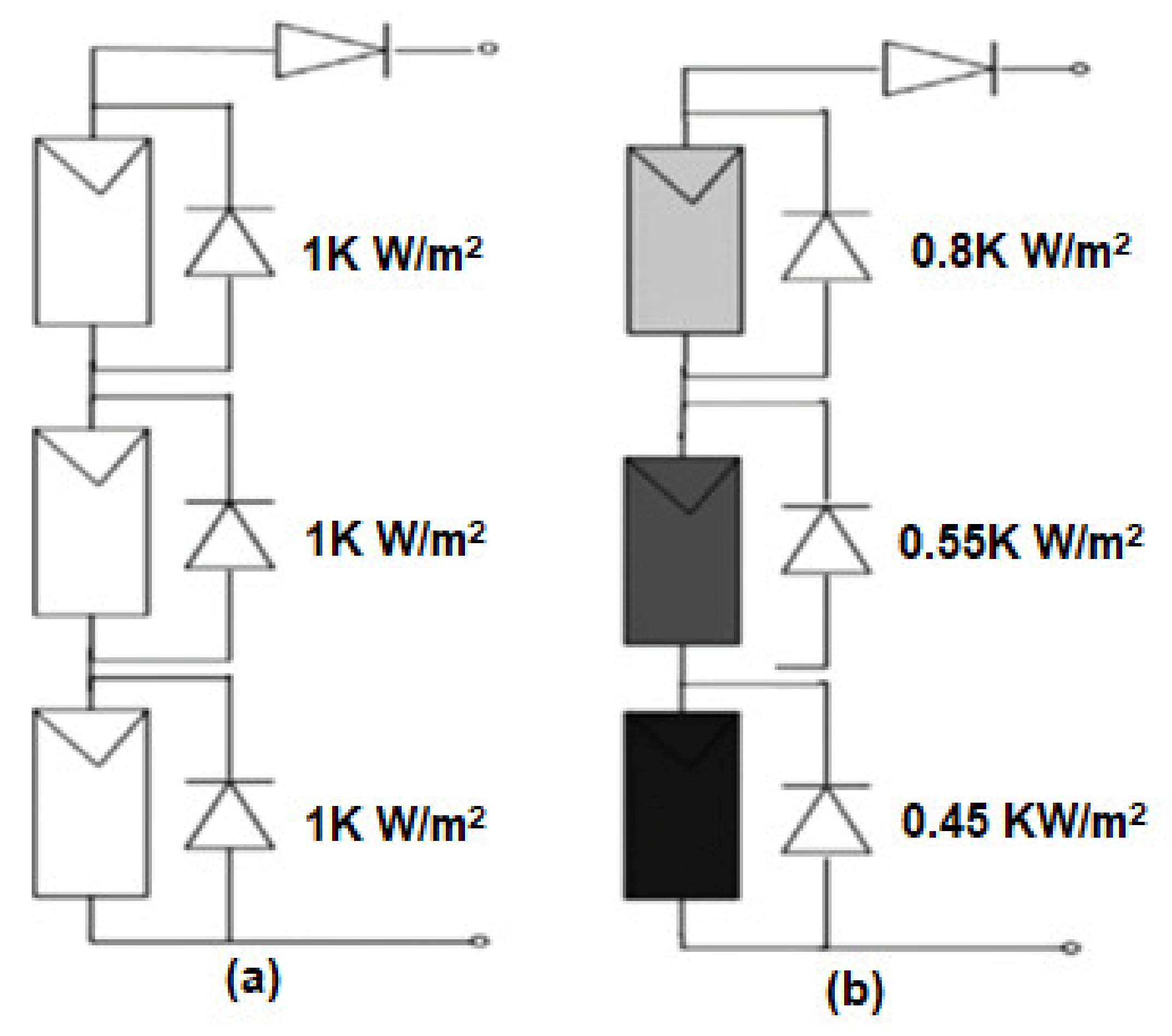
| PV Arrays Cases | Irradiance (W/m2) | Maximum Output Power | ||
|---|---|---|---|---|
| 1st Array | 2nd Array | 3rd Array | (W) | |
| Case-1 | 600 | 800 | 1000 | 9250 |
| Case-2 | 800 | 550 | 450 | 4240 |
| Symbol | Acronym |
|---|---|
| Separation of the ith individual dragonfly | |
| Alignment of the ith individual dragonfly | |
| Cohesion of the ith individual dragonfly | |
| Food attraction | |
| Enemy position | |
| Step size of DF movement | |
| w | Inertial weight |
| a | Separation weight |
| b | Alignment weight |
| b | Cohesion weight |
| d | Food factor |
| e | Enemy factor |
| Parameter | Symbol | Value |
|---|---|---|
| Quantity of particles | k | 4 |
| Separation weight | a | 0.2 |
| Alignment weight | b | 0.1 |
| Cohesion constant | c | 0.9 |
| Food factor | d | 0.5 |
| Enemy constant | e | 1 |
| MPPT Techniques | Sensed Variables | Steady State Error | Tracking Speed | GMPP Tracking | Tracking Accuracy | Efficiency | Complexity | Cost |
|---|---|---|---|---|---|---|---|---|
| P&O | V, I | High | Fast | No | Low | Less | Low | Cheap |
| PSO | V, I | Moderate | Fast | Yes | Medium | High | Medium | Moderate |
| ACSO | V, I | Less | Fast | Yes | High | High | High | Expensive |
| IPSO | V, I | Less | Fast | Yes | High | High | High | Expensive |
| FFO-GRNN | V, I | Less | Fast | Yes | High | High | High | Expensive |
| DOA | V, I | Less | Fast | Yes | High | High | High | Expensive |
| MPPT Techniques | Irradiance Cases | Converge Time (s) | Max Traced Power (W) | Global Max Power (W) | Global MPP Located | MPPT Accuracy | Percent Error |
|---|---|---|---|---|---|---|---|
| P&O | Case-1 | 0.18 | 5196 | 9250 | No | 56.17% | 43.82% |
| Case-2 | 0.12 | 2216 | 4240 | No | 52.26% | 47.73% | |
| PSO | Case-1 | 0.48 | 8767 | 9250 | Yes | 94.77% | 5.22% |
| Case-2 | 0.44 | 3948 | 4240 | Yes | 93.11% | 6.88% | |
| ACSO | Case-1 | 0.46 | 8889 | 9250 | Yes | 96.09% | 3.91% |
| Case-2 | 0.33 | 3979 | 4240 | Yes | 93.84% | 6.16% | |
| IPSO | Case-1 | 0.38 | 8982 | 9250 | Yes | 97.10% | 2.89% |
| Case-2 | 0.35 | 4032 | 4240 | Yes | 95.09% | 4.90% | |
| FFO-GRNN | Case-1 | 0.33 | 9003 | 9250 | Yes | 97.32% | 2.68% |
| Case-2 | 0.30 | 4094 | 4240 | Yes | 96.62% | 3.38% | |
| DOA | Case-1 | 0.29 | 9189 | 9250 | Yes | 99.34% | 0.65% |
| Case-2 | 0.32 | 4211 | 4240 | Yes | 99.31% | 0.68% |
Publisher’s Note: MDPI stays neutral with regard to jurisdictional claims in published maps and institutional affiliations. |
© 2021 by the authors. Licensee MDPI, Basel, Switzerland. This article is an open access article distributed under the terms and conditions of the Creative Commons Attribution (CC BY) license (https://creativecommons.org/licenses/by/4.0/).
Share and Cite
Lodhi, E.; Wang, F.-Y.; Xiong, G.; Mallah, G.A.; Javed, M.Y.; Tamir, T.S.; Gao, D.W. A Dragonfly Optimization Algorithm for Extracting Maximum Power of Grid-Interfaced PV Systems. Sustainability 2021, 13, 10778. https://0-doi-org.brum.beds.ac.uk/10.3390/su131910778
Lodhi E, Wang F-Y, Xiong G, Mallah GA, Javed MY, Tamir TS, Gao DW. A Dragonfly Optimization Algorithm for Extracting Maximum Power of Grid-Interfaced PV Systems. Sustainability. 2021; 13(19):10778. https://0-doi-org.brum.beds.ac.uk/10.3390/su131910778
Chicago/Turabian StyleLodhi, Ehtisham, Fei-Yue Wang, Gang Xiong, Ghulam Ali Mallah, Muhammad Yaqoob Javed, Tariku Sinshaw Tamir, and David Wenzhong Gao. 2021. "A Dragonfly Optimization Algorithm for Extracting Maximum Power of Grid-Interfaced PV Systems" Sustainability 13, no. 19: 10778. https://0-doi-org.brum.beds.ac.uk/10.3390/su131910778