
Deep Drilling for Groundwater in Bengaluru, India: A Case Study on the City’s Over-Exploited Hard-Rock Aquifer System


Abstract
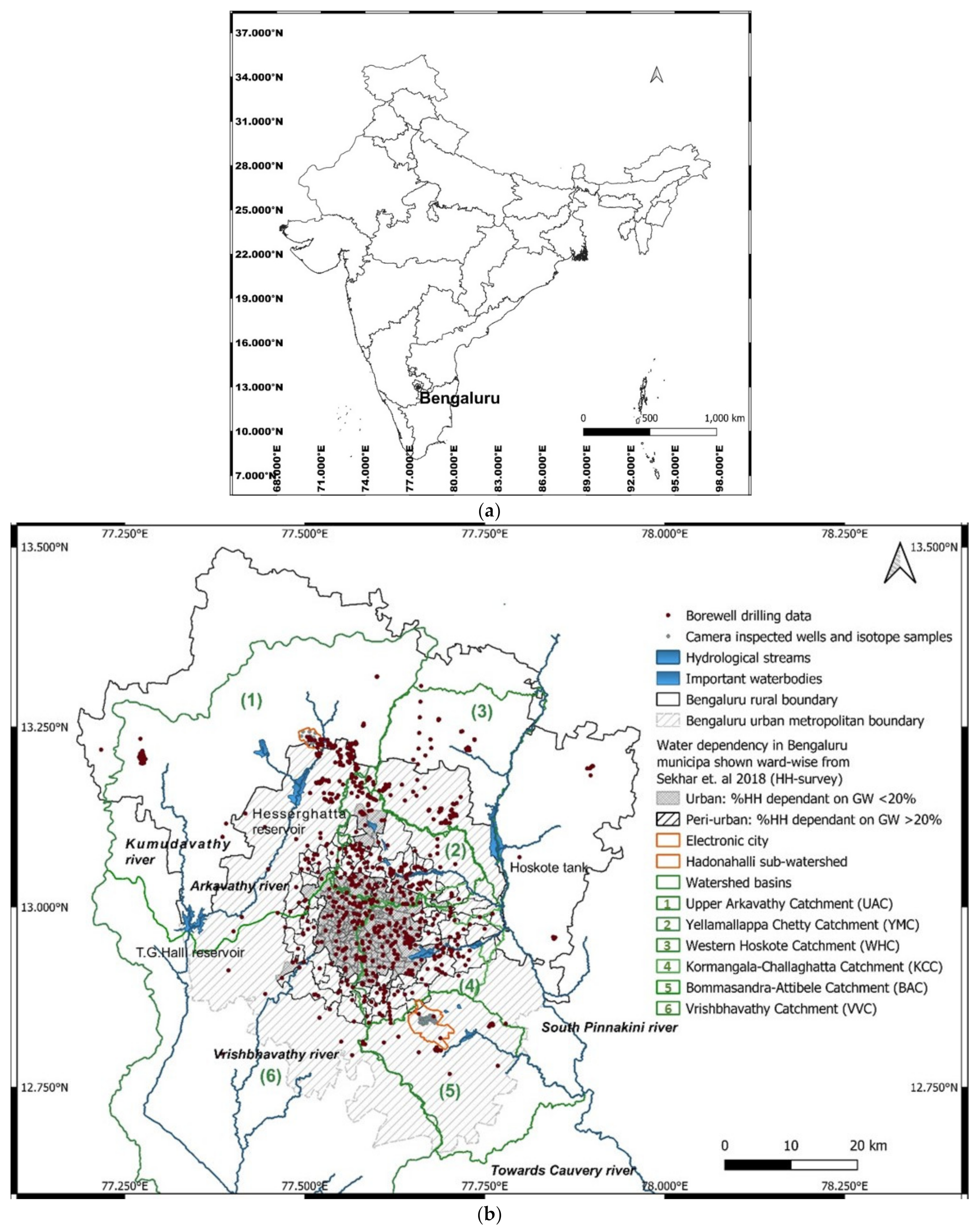
:1. Introduction
2. Materials and Methods
2.1. Reproducing Historical Groundwater Table Development of Bengaluru City
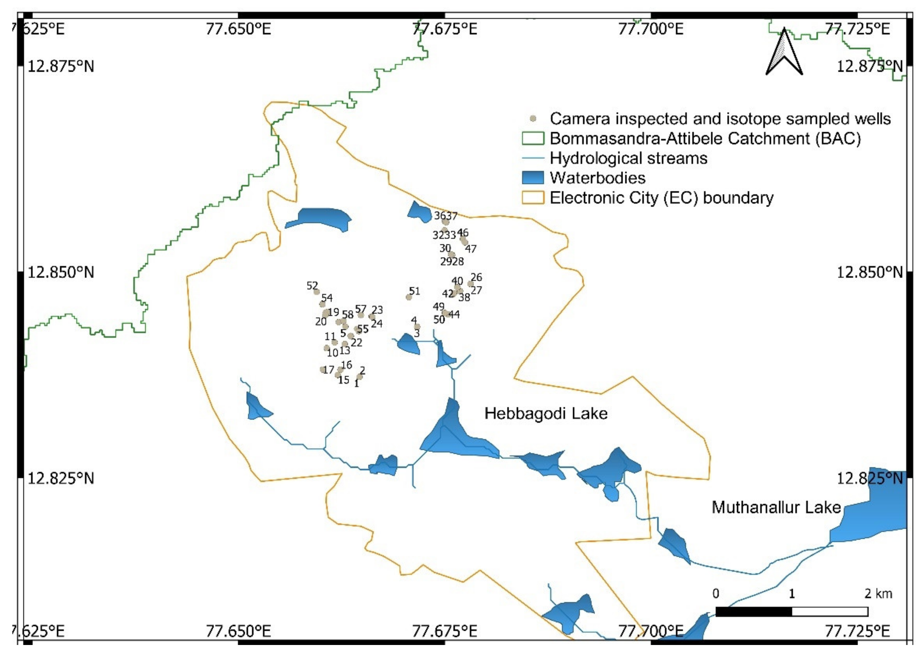
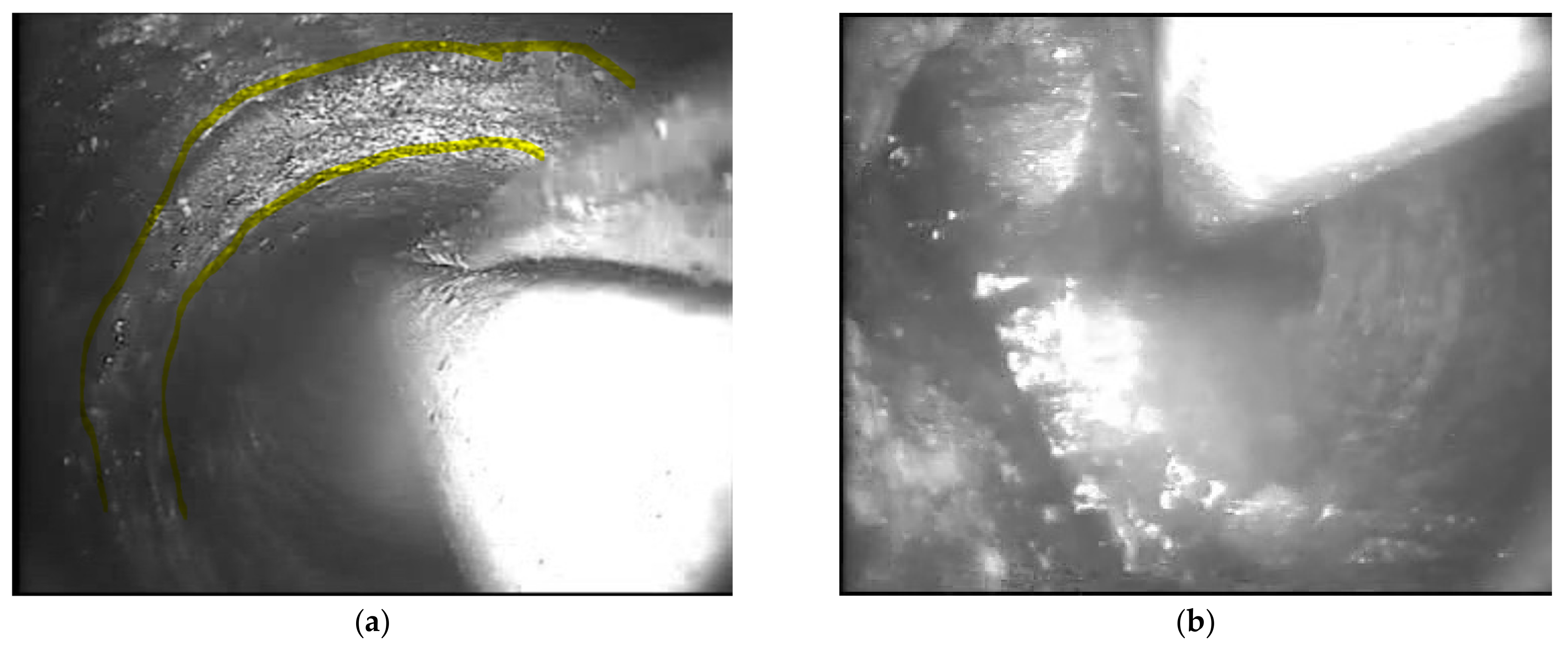
2.2. Aquifer Characterization through Hydrogeological Investigations by Camera Inspection
2.3. Hydro-Geochemical Investigations Using Stable Isotopes
3. Results and Discussions
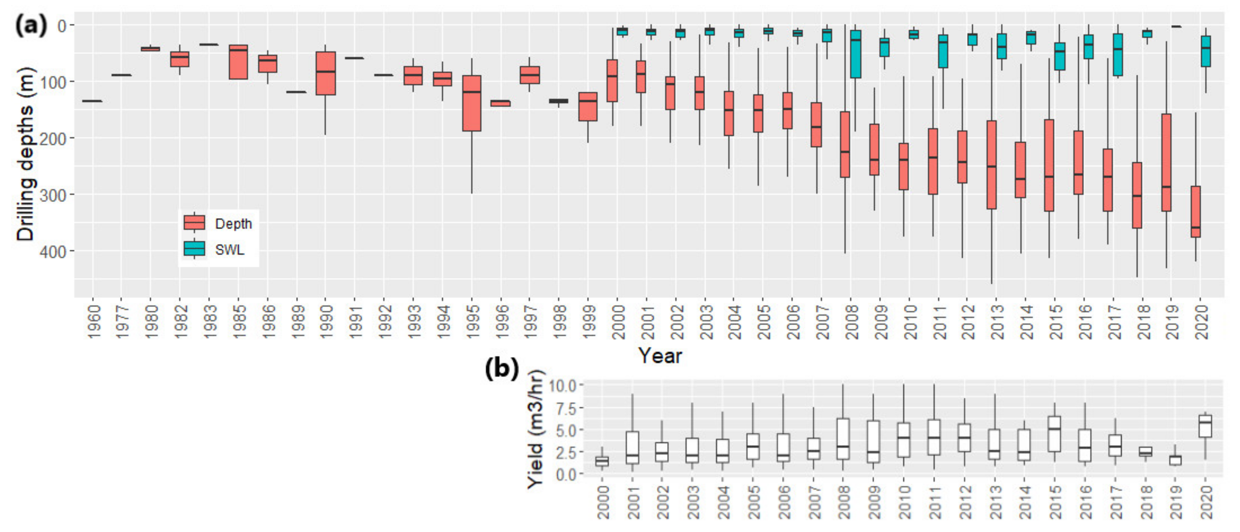
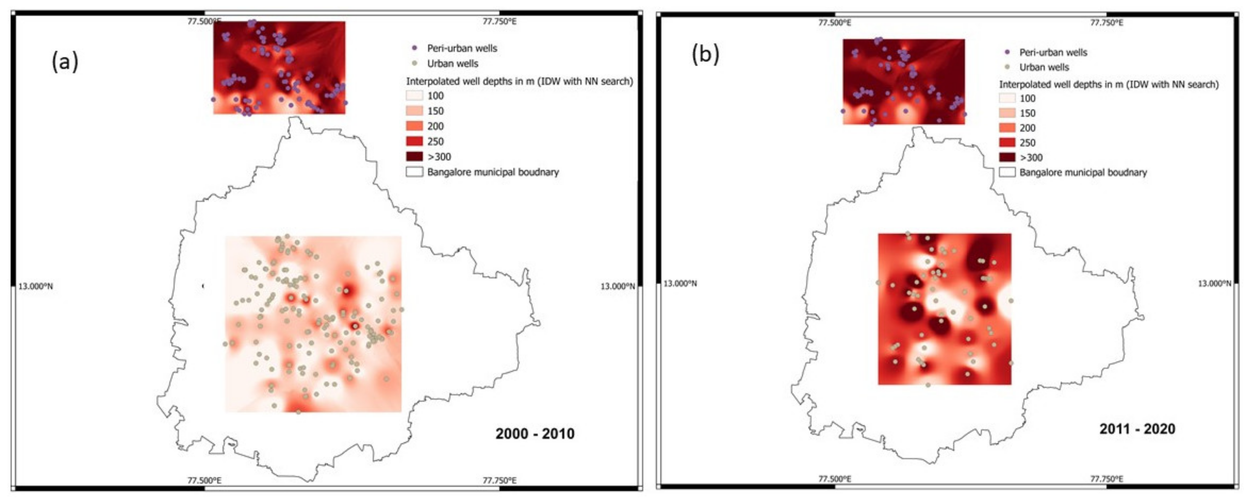
3.1. Spatio-Temporal Trends in Borewell and Groundwater Table Depths in Bengaluru City
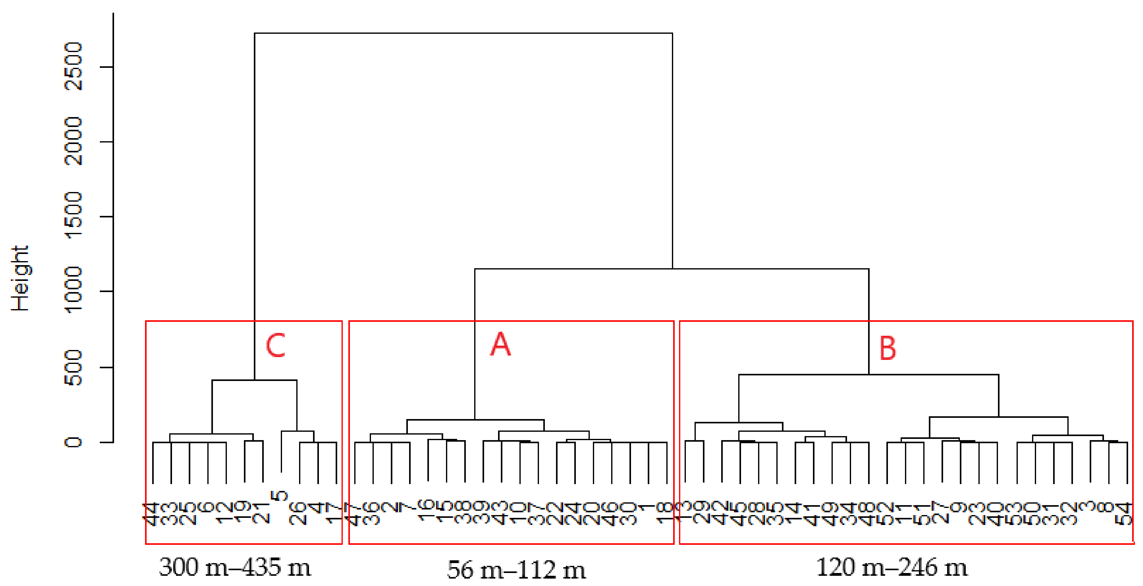
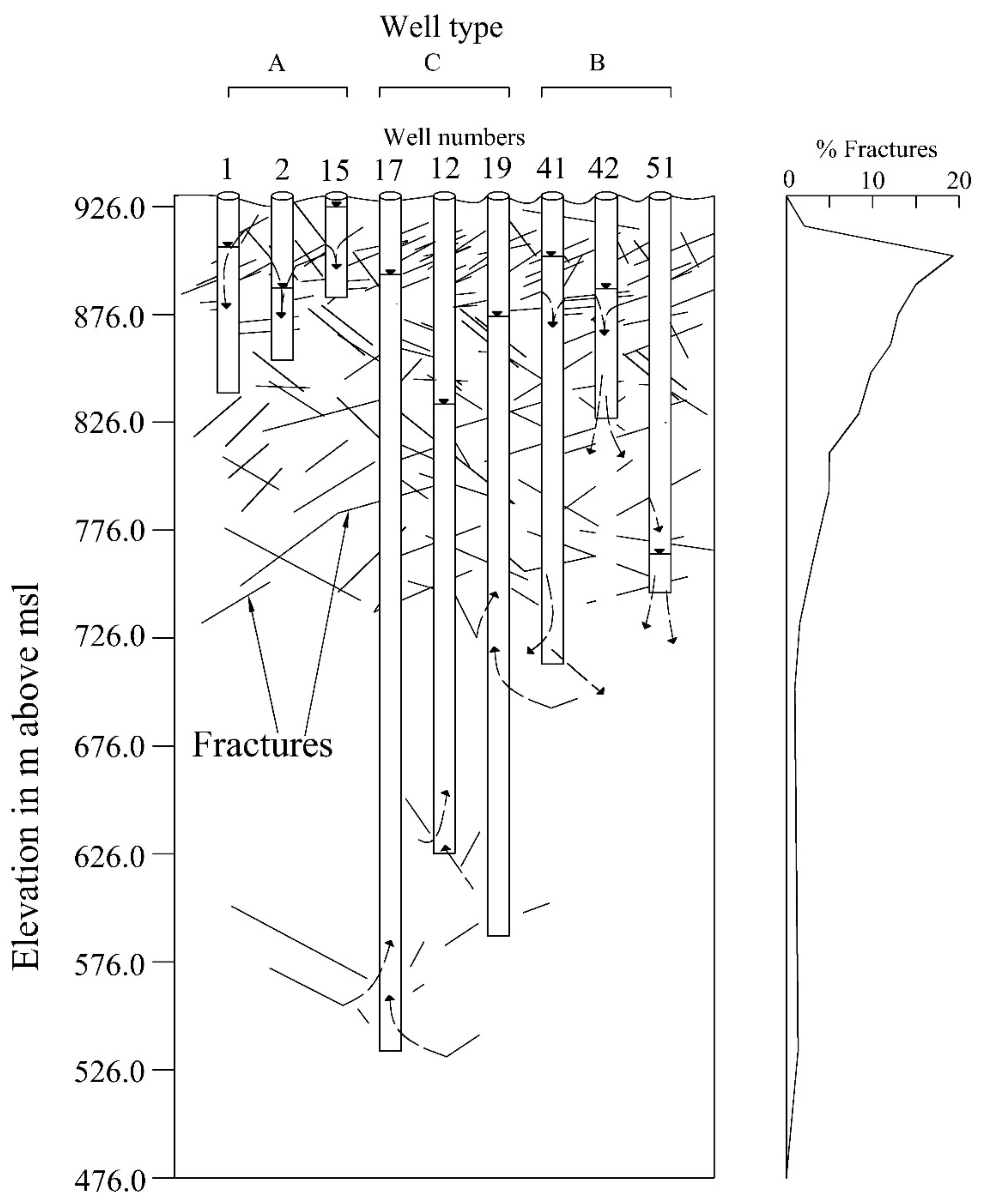
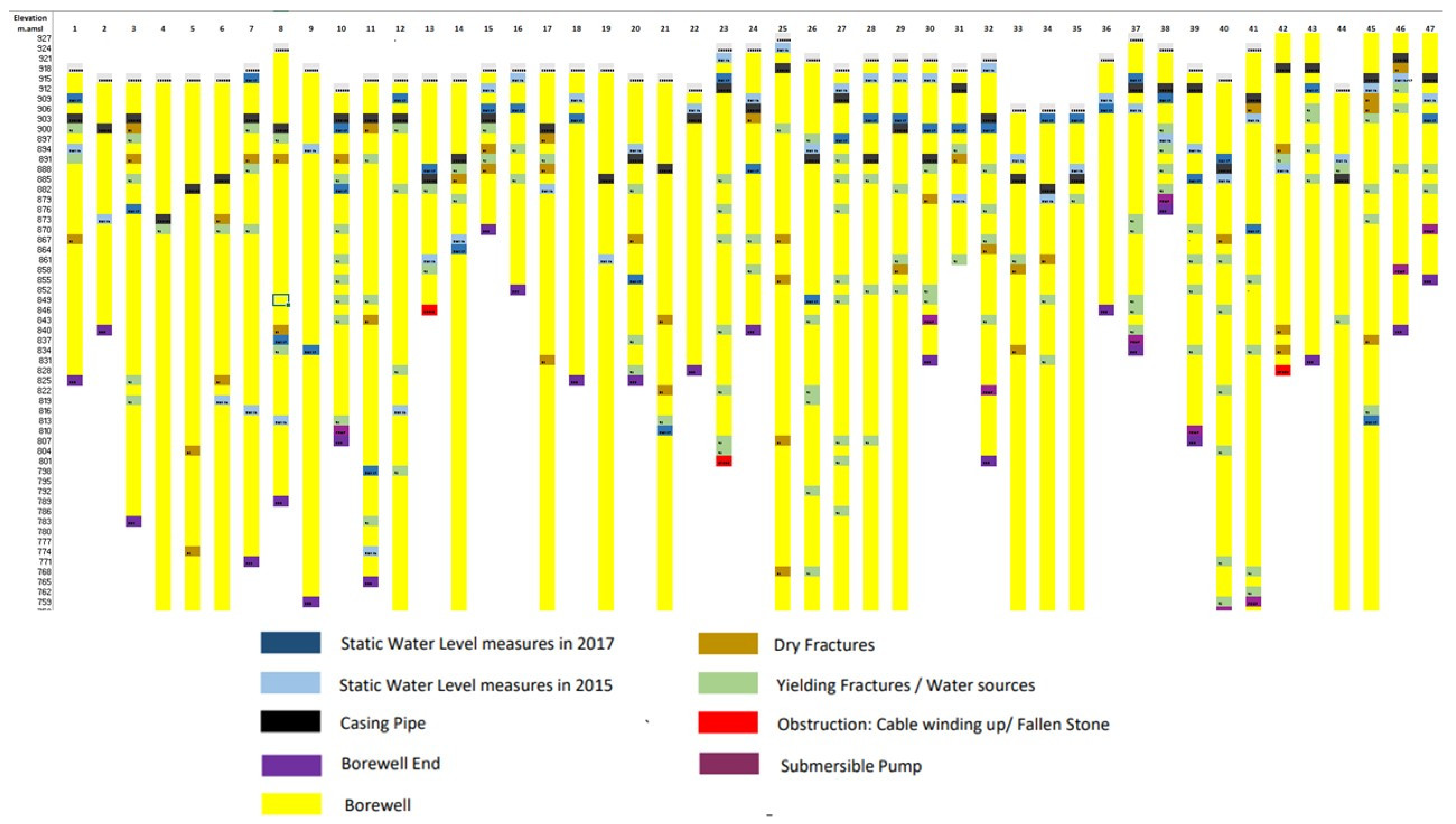
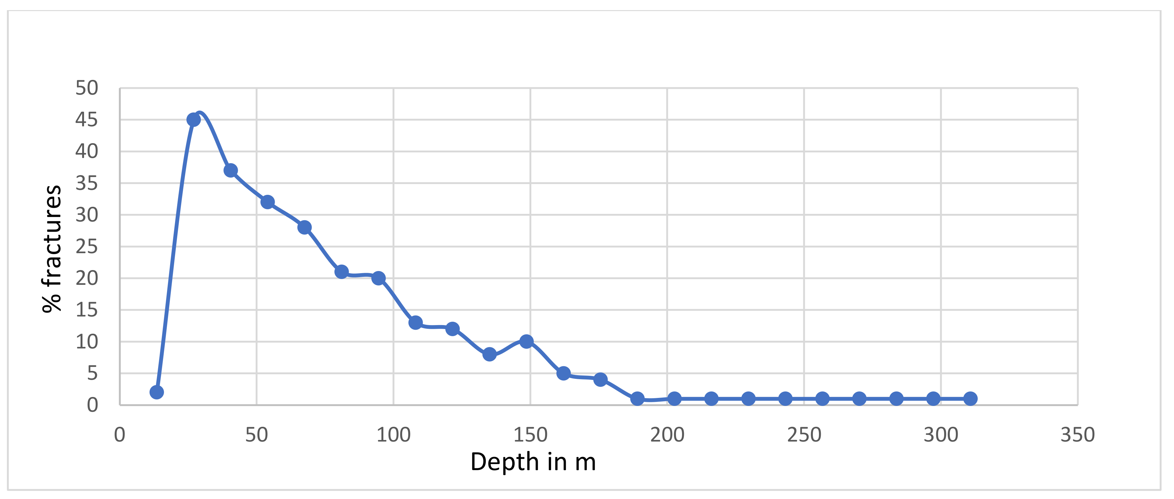
3.2. Aquifer Conceptualization at Electronic City, Bengaluru
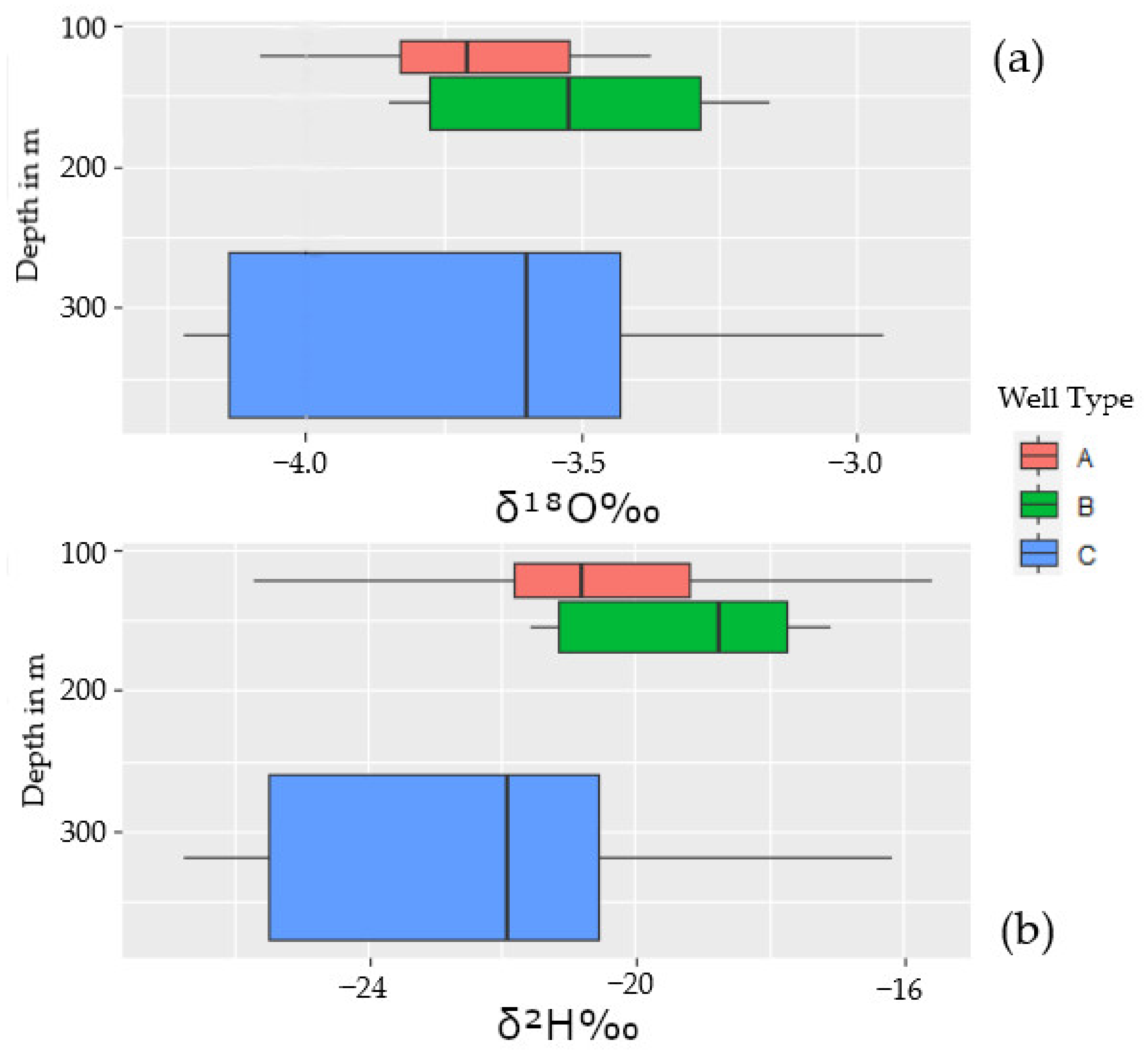
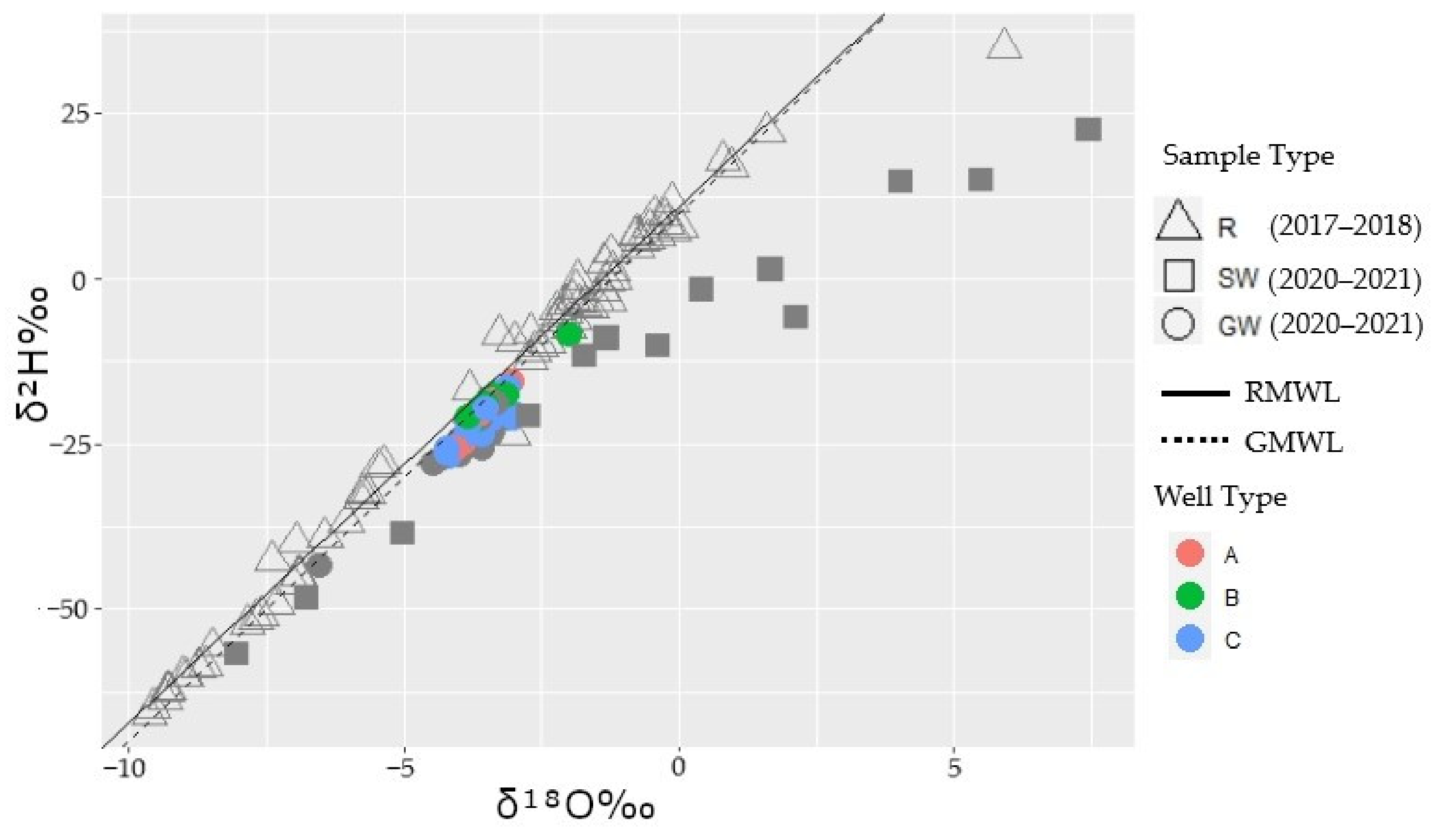
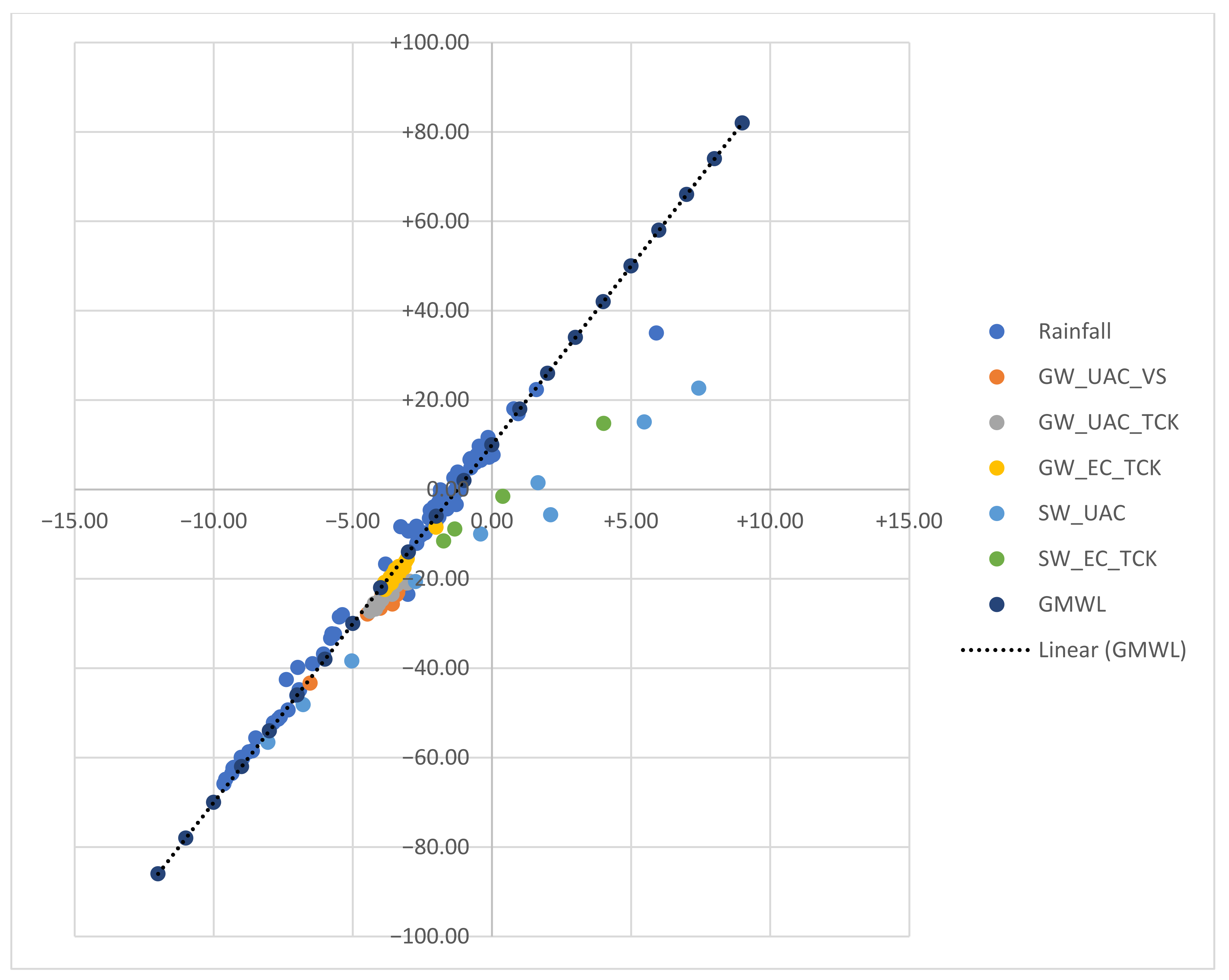
3.3. Hydro-Geochemical Analysis of Stable Isotopes in Water
3.4. Strengths and Limitations of the Study
4. Conclusions
Supplementary Materials
Author Contributions
Funding
Data Availability Statement
Acknowledgments
Conflicts of Interest
Appendix A


| Well No. | LAT | LON | Elevation | Catchment | Depth (m) | Well Type | Yielding Fractures below 245m | SWL 2016 m.bgl | SWL 2017 m.bgl | d_18O | d_2H | Selection for Further Monitoring |
|---|---|---|---|---|---|---|---|---|---|---|---|---|
| 1 | 12.84056 | 77.66333 | 918.02 | EC | 90.09 | A | - | 9.9 | 23.4 | −3.61 | −20.94 | No |
| 2 | 12.84667 | 77.65944 | 914.11 | EC | 75.08 | A | - | - | 42.0 | −3.79 | −21.54 | No |
| 3 | 12.85028 | 77.65778 | 915.92 | EC | 132.13 | B | - | 39.0 | 0.0 | - | - | No |
| 4 | 12.85222 | 77.65861 | 915.62 | EC | 390.39 | C | - | - | 287.1 | −3.83 | −21.43 | No |
| 5 | 12.85250 | 77.65889 | 915.62 | EC | 437.84 | C | 290 m | 227.0 | 326.0 | −3.80 | −21.21 | Yes |
| 6 | 12.85278 | 77.65972 | 915.62 | EC | 300.30 | C | 256 m | 212.0 | 95.1 | −3.84 | −21.58 | Yes |
| 7 | 12.84361 | 77.66222 | 919.22 | EC | 75.08 | A | - | 4.5 | 101.8 | −3.71 | −20.81 | No |
| 8 | 12.84722 | 77.65972 | 924.62 | EC | 135.14 | B | - | 88.6 | 111.1 | −3.82 | −22.05 | No |
| 9 | 12.84306 | 77.66278 | 918.62 | EC | 159.16 | B | - | 84.1 | 22.6 | −3.66 | −19.69 | No |
| 10 | 12.84306 | 77.66444 | 913.81 | EC | 104.20 | A | - | 13.5 | 28.8 | −3.81 | −21.39 | No |
| 11 | 12.84389 | 77.66333 | 915.92 | EC | 150.15 | B | - | 118.6 | 142.3 | −3.29 | −17.31 | No |
| 12 | 12.84361 | 77.66361 | 915.92 | EC | 300.30 | C | 246 m | 5.7 | 99.1 | −3.04 | −15.53 | Yes |
| 13 | 12.84444 | 77.66611 | 914.41 | EC | NA | - | - | 25.5 | 52.3 | −3.88 | −21.20 | No |
| 14 | 12.84444 | 77.66611 | 914.71 | EC | 210.21 | B | - | 49.5 | 46.8 | −3.47 | −17.94 | No |
| 15 | 12.84583 | 77.66778 | 918.02 | EC | 45.05 | A | - | 11.4 | 5.0 | −3.54 | −19.04 | No |
| 16 | 12.84667 | 77.66639 | 918.02 | EC | 63.06 | A | - | 9.6 | 3.0 | −3.35 | −17.24 | No |
| 17 | 12.84694 | 77.66972 | 917.12 | EC | 390.39 | C | - | 235.7 | 36.0 | −3.41 | −17.77 | No |
| 18 | 12.84667 | 77.66917 | 918.02 | EC | 90.09 | B | - | 15.0 | 9.0 | −3.25 | −17.08 | No |
| 19 | 12.84722 | 77.66889 | 918.62 | EC | 330.33 | C | - | 249.8 | 55.0 | −3.54 | −18.76 | No |
| 20 | 12.84639 | 77.67028 | 915.32 | EC | 87.69 | A | - | 60.1 | 19.8 | −3.39 | −17.78 | No |
| 21 | 12.84639 | 77.67056 | 914.11 | EC | 317.42 | C | - | 101.5 | 0.0 | - | - | No |
| 22 | 12.84583 | 77.67056 | 913.21 | EC | 84.08 | A | - | 5.1 | −2.01 | −8.47 | No | |
| 23 | 12.83639 | 77.65778 | 924.02 | EC | NA | - | - | 7.5 | 2.3 | −3.30 | −17.77 | No |
| 24 | 12.83694 | 77.66028 | 924.62 | EC | 84.08 | A | - | 36.0 | 14.4 | −3.44 | −19.49 | No |
| 25 | 12.83861 | 77.66250 | 927.63 | EC | 300.30 | C | 246 m | 189.2 | 3.6 | −3.10 | −16.14 | Yes |
| 26 | 12.83861 | 77.65361 | 921.02 | EC | 390.39 | C | 324 m | 70.6 | 25.3 | −3.40 | −18.68 | Yes |
| 27 | 12.83528 | 77.66167 | 919.52 | EC | 165.17 | B | - | 22.5 | 7.8 | −3.29 | −17.87 | No |
| 28 | 12.83583 | 77.66250 | 921.02 | EC | 180.18 | B | - | 18.0 | 6.0 | −3.26 | −17.74 | No |
| 29 | 12.83667 | 77.66222 | 922.22 | EC | 246.25 | C | - | 16.5 | 6.9 | −3.56 | −19.33 | No |
| 30 | 12.83611 | 77.66306 | 921.32 | EC | 90.09 | A | - | 18.6 | 6.6 | −3.61 | −19.51 | No |
| 31 | 12.83722 | 77.66500 | 920.12 | EC | 120.12 | B | - | 19.5 | 38.4 | −3.77 | −21.43 | No |
| 32 | 12.83639 | 77.66417 | 922.52 | EC | 120.12 | B | - | 22.5 | 0.0 | - | - | No |
| 33 | 12.84167 | 77.66722 | 907.81 | EC | 300.30 | C | 268 m | 180.8 | 16.5 | −3.75 | −21.58 | Yes |
| 34 | 12.84167 | 77.66694 | 908.41 | EC | 195.20 | B | - | 24.6 | −3.65 | −20.54 | No | |
| 35 | 12.84139 | 77.66806 | 907.21 | EC | 180.18 | B | - | 16.5 | −3.84 | −22.39 | No | |
| 36 | 12.83972 | 77.66361 | 923.42 | EC | 75.08 | A | - | 16.5 | 15.6 | −3.85 | −20.79 | No |
| 37 | 12.83806 | 77.66222 | 927.63 | EC | 105.11 | A | - | 12.0 | 21.0 | −3.16 | −17.55 | No |
| 38 | 12.83778 | 77.66194 | 925.83 | EC | 54.05 | A | - | 16.5 | 27.3 | −3.34 | −18.84 | No |
| 39 | 12.84194 | 77.66361 | 919.52 | EC | 111.11 | A | - | 33.3 | 24.0 | −3.52 | −18.78 | No |
| 40 | 12.84250 | 77.66444 | 915.32 | EC | 162.16 | B | - | 24.0 | 27.6 | −3.52 | −19.51 | No |
| 41 | 12.84139 | 77.66250 | 926.73 | EC | 210.21 | B | - | 54.1 | 22.8 | - | - | No |
| 42 | 12.84056 | 77.66056 | 932.43 | EC | 174.17 | B | - | - | 43.8 | - | - | No |
| 43 | 12.84056 | 77.66028 | 932.73 | EC | 100.60 | A | - | 20.7 | 0.0 | - | - | No |
| 44 | 12.84417 | 77.66472 | 914.41 | EC | 300.30 | C | - | - | 21.3 | −3.37 | −21.16 | No |
| 45 | 12.83972 | 77.65944 | 932.13 | EC | 180.18 | B | - | 117.1 | 16.8 | −3.37 | −18.08 | No |
| 46 | 12.83972 | 77.66000 | 932.73 | EC | 90.09 | A | - | 15.0 | 15.0 | −3.77 | −18.15 | No |
| 47 | 12.83944 | 77.65889 | 930.63 | EC | 75.08 | A | - | 27.6 | 21.0 | - | - | No |
| 48 | 12.83917 | 77.65917 | 930.33 | EC | 195.20 | B | - | 106.6 | 118.0 | - | - | No |
| 49 | 12.84000 | 77.65972 | 932.43 | EC | 195.20 | B | - | 127.6 | 84.4 | - | - | No |
| 50 | 12.84167 | 77.65972 | 929.73 | EC | 120.12 | B | - | 34.5 | 10.5 | - | - | No |
| 51 | 12.84194 | 77.67361 | 899.10 | EC | 150.15 | B | - | 131.5 | 0.0 | - | - | No |
| 52 | 12.84361 | 77.67250 | 901.50 | EC | NA | - | - | 0.0 | - | - | No | |
| 53 | 12.84361 | 77.66583 | 910.81 | EC | 120.12 | B | - | 12.0 | 36.0 | - | - | No |
| 54 | 12.84389 | 77.66583 | 912.01 | EC | 0.00 | - | - | 12.0 | - | - | - | No |
| 55 | 13.37326 | 77.54279 | 921.45 | UAC | 300.30 | C | - | - | - | −4.18 | −26.77 | Yes |
| 56 | 13.37467 | 77.54362 | 921.51 | UAC | 330.33 | C | - | - | - | −4.14 | −25.72 | - |
| 57 | 13.37457 | 77.54628 | 921.57 | UAC | 291.29 | C | - | - | - | −4.17 | −25.61 | - |
| 58 | 13.37685 | 77.54425 | 921.63 | UAC | 300.30 | C | - | - | - | −3.95 | −24.73 | - |
| 59 | 13.37647 | 77.54704 | 921.69 | UAC | 300.30 | C | - | - | - | −3.99 | −24.72 | - |
| 60 | 13.37504 | 77.54667 | 921.75 | UAC | 285.29 | C | - | - | - | −3.59 | −23.47 | - |
| 61 | 13.37619 | 77.54893 | 921.81 | UAC | 204.20 | C | - | - | - | −4.08 | −25.73 | - |
| 62 | 13.37495 | 77.55093 | 921.87 | UAC | 258.26 | C | - | - | - | −3.33 | −19.71 | - |
| 63 | 13.37559 | 77.54523 | 921.93 | UAC | 288.29 | C | - | - | - | −3.43 | −21.40 | - |
| 64 | 13.37176 | 77.54237 | 921.99 | UAC | 273.27 | C | - | - | - | −2.95 | −20.55 | - |
| 65 | 13.37908 | 77.54788 | 922.05 | UAC | 258.26 | C | - | - | - | −3.03 | −20.95 | - |
| 66 | 13.37936 | 77.54912 | 922.11 | UAC | 282.28 | C | - | - | - | −4.38 | −27.29 | - |
| 67 | 13.37880 | 77.54986 | 922.17 | UAC | 264.26 | C | - | - | - | −3.60 | −21.93 | - |
| 68 | 13.37808 | 77.55135 | 922.23 | UAC | 270.27 | C | - | - | - | −4.22 | −26.28 | - |
| 69 | 13.37815 | 77.55211 | 922.29 | UAC | 324.32 | C | - | - | - | −4.22 | −25.49 | - |
References
- McDonald, R.I.; Weber, K.; Padowski, J.; Flörke, M.; Schneider, C.; Green, P.A.; Gleeson, T.; Eckman, S.; Lehner, B.; Balk, D.; et al. Water on an Urban Planet: Urbanization and the Reach of Urban Water Infrastructure. Glob. Environ. Change 2014, 27, 96–105. [Google Scholar] [CrossRef] [Green Version]
- Flörke, M.; Schneider, C.; McDonald, R.I. Water Competition between Cities and Agriculture Driven by Climate Change and Urban Growth. Nat. Sustain. 2018, 1, 51–58. [Google Scholar] [CrossRef]
- Schwartz, F.W.; Liu, G.; Yu, Z. HESS Opinions: The Myth of Groundwater Sustainability in Asia. Hydrol. Earth Syst. Sci. 2020, 24, 489–500. [Google Scholar] [CrossRef] [Green Version]
- Gleeson, T.; Cuthbert, M.; Ferguson, G.; Perrone, D. Global Groundwater Sustainability, Resources, and Systems in the Anthropocene. Annu. Rev. Earth Planet. Sci. 2020, 48, 431–463. [Google Scholar] [CrossRef] [Green Version]
- Bredehoeft, J.D. The Water Budget Myth Revisited: Why Hydrogeologists Model. Ground Water 2002, 40, 340–345. [Google Scholar] [CrossRef] [PubMed]
- Ferguson, G.; Cuthbert, M.O.; Befus, K.; Gleeson, T.; McIntosh, J.C. Rethinking Groundwater Age. Nat. Geosci. 2020, 13, 592–594. [Google Scholar] [CrossRef]
- Shah, T. Taming the Anarchy—Groundwater Governance in South Asia; Resources for the Future: Washington, USA, 2009; ISBN 978-1-933115-60-3. [Google Scholar]
- Groundwater of South Asia; Mukherjee, A. (Ed.) Springer: Singapore, 2018; ISBN 978-981-10-3888-4. [Google Scholar]
- Kulkarni, H.; Shankar, P.; Vijay, S. Groundwater Resources in India: An Arena for Diverse Competition. Local Environ. 2014, 19, 990–1011. [Google Scholar] [CrossRef]
- Shankar, P.V.; Kulkarni, H.; Krishnan, S. India’s Groundwater Challenge and the Way Forward. Econ. Polit. Wkly. 2011, 46, 37–45. [Google Scholar]
- Kulkarni, H.; Shah, M.; Vijay Shankar, P.S. Shaping the Contours of Groundwater Governance in India. J. Hydrol. Reg. Stud. 2015, 4, 172–192. [Google Scholar] [CrossRef] [Green Version]
- Arshad, I.; Umar, R. Status of Urban Hydrogeology Research with Emphasis on India. Hydrogeol. J. 2020, 28, 477–490. [Google Scholar] [CrossRef]
- Das, S. Frontiers of Hard Rock Hydrogeology in India. In Ground Water Development—Issues and Sustainable Solutions; Ray, S.P.S., Ed.; Springer: Singapore, 2019; ISBN 9789811317705. [Google Scholar]
- Srinivasan, V.; Thompson, S.; Madhyastha, K.; Penny, G.; Jeremiah, K.; Lele, S. Why Is the Arkavathy River Drying? A Multiple-Hypothesis Approach in a Data-Scarce Region. Hydrol. Earth Syst. Sci. 2015, 19, 1905–1917. [Google Scholar] [CrossRef] [Green Version]
- Sudhira, H.S.; Ramachandra, T.V.; Subrahmanya, M.H.B. Bangalore. Cities 2007, 24, 379–390. [Google Scholar] [CrossRef]
- Raj, K. Urbanization and Water Supply: An Analysis of Unreliable Water Supply in Bangalore City, India. In Nature, Economy and Society; Ghosh, N., Mukhopadhyay, P., Shah, A., Panda, M., Eds.; Springer: New Delhi, India, 2016; ISBN 978-81-322-2403-7. [Google Scholar]
- Patil, V.S.; Thomas, B.K.; Lele, S.; Eswar, M.; Srinivasan, V. Adapting or Chasing Water? Crop Choice and Farmers’ Responses to Water Stress in Peri-Urban Bangalore, India. Irrig. Drain. 2019, 68, 140–151. [Google Scholar] [CrossRef] [Green Version]
- Steinhübel, L.; Wegmann, J.; Mußhoff, O. Digging Deep and Running Dry—the Adoption of Borewell Technology in the Face of Climate Change and Urbanization. Agric. Econ. 2020, 51, 685–706. [Google Scholar] [CrossRef]
- Hora, T.; Srinivasan, V.; Basu, N.B. The Groundwater Recovery Paradox in South India. Geophys. Res. Lett. 2019, 46, 9602–9611. [Google Scholar] [CrossRef]
- Ballukraya, P.N.; Srinivasan, V. Sharp Variations in Groundwater Levels at the Same Location: A Case Study from Heavily Exploited, Fractured Rock Aquifer System near Bangalore, South India. Curr. Sci. 2019, 117, 130–138. [Google Scholar] [CrossRef]
- Thippiah, P. Water and environmental crisis in mega city: Vanishing lakes and over-exploited ground water in Bangalore. In Urban Governance in Karnataka and Bengaluru: Global Changes and Local Impacts; Cambridge Scholars: Newcastle upon Tyne, UK, 2009. [Google Scholar]
- Chandra, S.; Auken, E.; Maurya, P.K.; Ahmed, S.; Verma, S.K. Large Scale Mapping of Fractures and Groundwater Pathways in Crystalline Hardrock By AEM. Sci. Rep. 2019, 9, 398. [Google Scholar] [CrossRef] [PubMed] [Green Version]
- Saha, D.; Marwaha, S.; Dwivedi, S.N. National Aquifer Mapping and Management Programme: A Step Towards Water Security in India. In Water Governance: Challenges and Prospects; Singh, A., Saha, D., Tyagi, A.C., Eds.; Springer: Singapore, 2019; pp. 49–66. ISBN 9789811326998. [Google Scholar]
- Sekhar, M.; Mujumdar, P.P. Evaluation of Scheme of Ground Water Management & Regulation (2012-17); Department of Civil Engineering, Indian Institute of Scoences: Bangalore, India, 2017. [Google Scholar]
- Rangan, A.K. Participatory Groundwater Management: Lessons from Programmes Across India. IIM Kozhikode Soc. Manag. Rev. 2016, 5, 8–15. [Google Scholar] [CrossRef]
- Ghose, B.; Dhawan, H.; Kulkarni, H.; Aslekar, U.; Patil, S.; Ramachandrudu, M.V.; Cheela, B.; Jadeja, Y.; Thankar, B.; Chopra, R.; et al. Peoples’ Participation for Sustainable Groundwater Management. In Clean and Sustainable Groundwater in India; Saha, D., Marwaha, S., Mukherjee, A., Eds.; Springer: Singapore, 2018; ISBN 978-981-10-4551-6. [Google Scholar]
- Collins, S.L.; Loveless, S.E.; Muddu, S.; Buvaneshwari, S.; Palamakumbura, R.N.; Krabbendam, M.; Lapworth, D.J.; Jackson, C.R.; Gooddy, D.C.; Nara, S.N.V.; et al. Groundwater Connectivity of a Sheared Gneiss Aquifer in the Cauvery River Basin, India. Hydrogeol. J. 2020, 28, 1371–1388. [Google Scholar] [CrossRef] [Green Version]
- Srinivasan, V. Doing Science That Matters to Address India’s Water Crisis. Resonance 2017, 22, 303–313. [Google Scholar] [CrossRef]
- Hynds, P.; Regan, S.; Andrade, L.; Mooney, S.; O’Malley, K.; DiPelino, S.; O’Dwyer, J. Muddy Waters: Refining the Way Forward for the “Sustainability Science” of Socio-Hydrogeology. Water 2018, 10, 1111. [Google Scholar] [CrossRef] [Green Version]
- Hoffmann, E.; Jose, M.; Nölke, N.; Möckel, T. Construction and Use of a Simple Index of Urbanisation in the Rural–Urban Interface of Bangalore, India. Sustainability 2017, 9, 2146. [Google Scholar] [CrossRef] [Green Version]
- Wegmann, J.; Mußhoff, O. Groundwater Management Institutions in the Face of Rapid Urbanization – Results of a Framed Field Experiment in Bengaluru, India. Ecol. Econ. 2019, 166, 106432. [Google Scholar] [CrossRef]
- Sekhar, M.; Tomer, S.; Thiyaku, S.; Giriraj, P.; Murthy, S.; Mehta, V. Groundwater Level Dynamics in Bengaluru City, India. Sustainability 2018, 10, 26. [Google Scholar] [CrossRef] [Green Version]
- Hirsch, R.M.; Slack, J.R. A Nonparametric Trend Test for Seasonal Data With Serial Dependence. Water Resour. Res. 1984, 20, 727–732. [Google Scholar] [CrossRef] [Green Version]
- Mitas, L.; Mitasova, H. Spatial Interpolation. In Geographical Information Systems: Principles, Techniques, Management and Applications; Wiley: Chichester, UK, 1999. [Google Scholar]
- Van Dijk, M.P. Government Policies with Respect to an Information Technology Cluster in Bangalore, India. Eur. J. Dev. Res. 2003, 15, 93–108. [Google Scholar] [CrossRef]
- Heitzman, J. Corporate Strategy and Planning in the Science City: Bangalore as “Silicon Valley”. Econ. Polit. Wkly. 2021, 34, 11. [Google Scholar]
- Bala Subrahmanya, M.H. Innovation and Growth of Engineering SMEs in Bangalore: Why Do Only Some Innovate and Only Some Grow Faster? J. Eng. Technol. Manag. 2015, 36, 24–40. [Google Scholar] [CrossRef]
- Maechler, M.; Rosseeuw, P.; Struyf, A.; Hubert, M.; Hornik, K. Cluster: Cluster Analysis Basics and Extensions; R Foundation: Vienna, Austria, 2021. [Google Scholar]
- Deshpande, R.D. Isotope Tracer Applications in Groundwater Hydrology: A Review of Indian Scenario. In Groundwater of South Asia; Mukherjee, A., Ed.; Springer: Singapore, 2018; pp. 233–245. ISBN 978-981-10-3888-4. [Google Scholar]
- Gupta, S.K.; Deshpande, R.D. Groundwater Isotopic Investigations in India: What Has Been Learned? Curr. Sci. 2005, 89, 12. [Google Scholar]
- Penny, G.; Srinivasan, V.; Apoorva, R.; Jeremiah, K.; Peschel, J.; Young, S.; Thompson, S. A Process-based Approach to Attribution of Historical Streamflow Decline in a Data-scarce and Human-dominated Watershed. Hydrol. Process. 2020, 34, 1981–1995. [Google Scholar] [CrossRef]
- Dansgaard, W. Stable Isotopes in Precipitation. Tellus 1964, 16, 436–468. [Google Scholar] [CrossRef]
- Kumar, B.; Rai, S.P.; Kumar, U.S.; Verma, S.K.; Garg, P.; Kumar, S.V.V.; Jaiswal, R.; Purendra, B.K.; Kumar, S.R.; Pande, N.G. Isotopic Characteristics of Indian Precipitation. Water Resour. Res. 2010, 46, W12548. [Google Scholar] [CrossRef]
- Goldman, M.; Narayan, D. Water Crisis through the Analytic of Urban Transformation: An Analysis of Bangalore’s Hydrosocial Regimes. Water Int. 2019, 44, 95–114. [Google Scholar] [CrossRef]
- Tomer, S.K.; Sekhar, M.; Balakrishnan, K.; Malghan, D.; Thiyaku, S.; Gautam, M.; Mehta, V.K. A Model-Based Estimate of the Groundwater Budget and Associated Uncertainties in Bengaluru, India. Urban Water J. 2020, 18, 1–11. [Google Scholar] [CrossRef]
- Kumar, A.; Ramachandran, P. Cross-Sectional Study of Factors Influencing the Residential Water Demand in Bangalore. Urban Water J. 2019, 16, 171–182. [Google Scholar] [CrossRef]
- Castán Broto, V.; Sudhira, H.S.; Unnikrishnan, H. Walk the Pipeline: Urban Infrastructure Landscapes in Bengaluru’s Long Twentieth Century. Int. J. Urban Reg. Res. 2021, 45, 696–715. [Google Scholar] [CrossRef]
- Mehta, V.K.; Goswami, R.; Kemp-Benedict, E.; Malghan, D.; Muddu, S. Social Ecology of Domestic Water Use in Bangalore. Econ. Polit. Wkly. 2013, 48, 12. [Google Scholar]
- Yadav, B.; Gupta, P.K.; Patidar, N.; Himanshu, S.K. Ensemble Modelling Framework for Groundwater Level Prediction in Urban Areas of India. Sci. Total Environ. 2020, 712, 135539. [Google Scholar] [CrossRef] [PubMed]
- Chandrakanth, M.G. Water Resource Economics; Springer: New Delhi, India, 2015; ISBN 978-81-322-2478-5. [Google Scholar]
- Siddique, I.; Mahamuni, K.; Desai, J.; Patil, S.; Kulkarni, H. Hydrogeological Aspects of Paticipatory Aquifer Mapping (PAQM) in Urban Groundwater Scenario in South-East Bengaluru; Advanced Center for Water Resources Development and Management (ACWADAM): Bangalore, India, 2017; p. 79. [Google Scholar]
- Ramya, C. The Indian Megacity Digging a Million Wells, BBC 2020. Available online: https://www.bbc.com/future/article/20201006-india-why-bangalore-is-digging-a-million-wells (accessed on 30 October 2021).
- Rahul, P.; Ghosh, P. Long Term Observations on Stable Isotope Ratios in Rainwater Samples from Twin Stations over Southern India; Identifying the Role of Amount Effect, Moisture Source and Rainout during the Dual Monsoons. Clim. Dyn. 2019, 52, 6893–6907. [Google Scholar] [CrossRef]
- Kumar, S.; Sharma, S.; Navada, S.V.; Deodhar, A.S. Environmental Isotopes Investigation on Recharge Processes and Hydrodynamics of the Coastal Sedimentary Aquifers of Tiruvadanai, Tamilnadu State, India. J. Hydrol. 2009, 364, 23–39. [Google Scholar] [CrossRef]
- Wenninger, J. Handbook for Stable Isotope Data Interpretation in India; IHE Delft Institute for Water Education: Delft, The Netherlands, 2020. [Google Scholar]
- Singh, M.J.; Davis, D.; Somashekar, R.K.; Prakash, K.L.; Shivanna, K. Environmental Isotopes Investigation in Groundwater of Challaghatta Valley, Bangalore: A Case Study. Afr. J. Environ. Sci. Technol. 2010, 4, 226–233. [Google Scholar]
- Ramesh, M. The Climate Solution. India’s Climate-Change Crisis and What We Can Do about It; Hachette: Gurugram, India, 2018; ISBN 978-93-5195-232-9. [Google Scholar]


| Parameter | Time Period | Location Category | ||||||||
|---|---|---|---|---|---|---|---|---|---|---|
| Spatial | Valleys | |||||||||
| Urban | Peri-Urban | Rural | UAC | YMC | WHC | KCC | VVC | BAC | ||
| Drilling depth of borewells (m) | Pre-2000 | NA | 120.1 | 105.1 | 120.1 | 63.1 | 105.0 | NA | NA | 115 |
| 2000–2010 | 125 | 152.2 | 180.2 | 180.2 | 141 | 195 | 140 | 83 | 152 | |
| 2011–2020 | 211 | 264.6 | 301.8 | 300 | 261.3 | 300 | 198 | 188 | 331 | |
| Static water levels (m) | 2000–2010 | 12 | 15.0 | 23.8 | 15 | 43.3 | 50 | 15 | 18 | 13 |
| 2011–2020 | 18 | 29.0 | 46.4 | 36 | 35 | 38 | 15 | 16 | 76 | |
| Reported yield m3/h | 2000–2010 | 2.45 | 2.0 | 4.0 | 2.0 | 2 | 2.0 | 2 | 2 | 3.2 |
| 2011–2020 | 3.5 | 4 | 3.9 | 2 | 2.75 | NA | 3.4 | 3.5 | 3.5 | |
| Parameter | Time Period | Mann–Kendall Trend Analysis—Sen’s Slope | ||||||||
|---|---|---|---|---|---|---|---|---|---|---|
| Spatial | Valleys | |||||||||
| Urban | Peri-Urban | Rural | UAC | YMC | WHC | KCC | VVC | BAC | ||
| Rise in drilling depth of borewells (m/year) | Pre-2000 | NA | 3 | 6 | 7 | NA | 3.30 | NA | NA | NA |
| 2000–2010 | 13.0 | 15.4 | 16.9 | 17.1 | 4.9 | 13.5 | 15.4 | 12 | 11.25 | |
| 2011–2020 | 5.6 | 12.3 | 7.5 | 6.1 | 8.5 | 2.6 | 4.2 | n.s. | n.s. | |
| 1960–2020 | 10.7 | 7.4 | 9.0 | 9.3 | 8.0 | 7.1 | 8.3 | 8.5 | 9.70 | |
Publisher’s Note: MDPI stays neutral with regard to jurisdictional claims in published maps and institutional affiliations. |
© 2021 by the authors. Licensee MDPI, Basel, Switzerland. This article is an open access article distributed under the terms and conditions of the Creative Commons Attribution (CC BY) license (https://creativecommons.org/licenses/by/4.0/).
Share and Cite
Kulkarni, T.; Gassmann, M.; Kulkarni, C.M.; Khed, V.; Buerkert, A. Deep Drilling for Groundwater in Bengaluru, India: A Case Study on the City’s Over-Exploited Hard-Rock Aquifer System. Sustainability 2021, 13, 12149. https://0-doi-org.brum.beds.ac.uk/10.3390/su132112149
Kulkarni T, Gassmann M, Kulkarni CM, Khed V, Buerkert A. Deep Drilling for Groundwater in Bengaluru, India: A Case Study on the City’s Over-Exploited Hard-Rock Aquifer System. Sustainability. 2021; 13(21):12149. https://0-doi-org.brum.beds.ac.uk/10.3390/su132112149
Chicago/Turabian StyleKulkarni, Tejas, Matthias Gassmann, C. M. Kulkarni, Vijayalaxmi Khed, and Andreas Buerkert. 2021. "Deep Drilling for Groundwater in Bengaluru, India: A Case Study on the City’s Over-Exploited Hard-Rock Aquifer System" Sustainability 13, no. 21: 12149. https://0-doi-org.brum.beds.ac.uk/10.3390/su132112149