Soil Available Phosphorus Investigated for Spatial Distribution and Effect Indicators Resulting from Ecological Construction on the Loess Plateau, China

Abstract

Soil phosphorus is a major determinant and indicator of soil fertility and quality, and is also a source of nonpoint-source pollution. In order to control soil and water loss in the Loess Plateau, a series of soil and water conservation measures have been taken, resulting in changes in land use and differences in spatial distribution. It is necessary to study soil available phosphorus (SAP) to evaluate land productivity and environmental quality. In this study, the spatial distribution of SAP in different land uses was investigated in a small catchment area of Loess Plateau, and the field-influencing factors were determined on five layers with soil depth of 20 cm. The results show the minimum and maximum SAP content occurred at 20–40 cm and 80–100 cm soil depth and reach a value of 27.26 mg/kg and 29.37 mg/kg at catchment scale, respectively. There is significant difference among the SAP of the five soil layers (p < 0.01). The SAP of different land uses is, in order: forestland < slope farmland < dam farmland < terrace < grassland. Different land uses’ topographies make a difference to the spatial distribution of SAP. Slope and soil texture are the domain factors influencing the SAP concentration at the catchment.

1. Introduction

As an important part of the soil, phosphorus is an extremely important ecological factor in terrestrial and aquatic ecosystems, and also a necessary nutrient element for the life activities of animals and plants [1]. In terrestrial ecosystems, the soil phosphorus level is closely related to soil productivity, for it directly affects soil fertility and crop growth quality. Availability of phosphorus (P) can directly and/or indirectly affect nitrogen (N) retention and loss from soil by stimulating microbial and plant root activities [2]. In recent years in the agricultural ecosystem, in order to increase soil fertility and increase crop yields, a large amount of chemical fertilizers has been artificially thrown into the soil, which has in essence led to the enrichment of phosphorus in terrestrial ecosystems [3]. Excessive enrichment of phosphorus can change the effectiveness of nutrients and increase the number and activity of microorganisms [4]. At the same time, large amounts of phosphorus emitted due to agricultural production causes water eutrophication [5,6], endangering the water supply ecosystem and human health. Land use changes caused by human factors and climate change also have important impacts on the content changes of soil available phosphorus (SAP). Changes in land use patterns often lead to changes in the soil phosphorus cycle pattern, affecting the stability and sustainability of the entire ecosystem [7]. Irrational land use can lead to serious soil erosion and environmental problems, for instance, water eutrophication arising from the loss of soil nutrients [8]. In the meanwhile, frequent changes in land use structure will also conflict with the ecological environment [9], resulting in a series of serious consequences, such as increasing soil loss; reducing the content of organic matter, nitrogen, and phosphorus in soil; as well as impairing soil fertility [10]. Plant cover significantly reduced available P losses in experimental fields [11]. However, appropriate soil and water conservation measures can significantly decrease soil erosion and nutrient loss, especially in the Loess Plateau, which is ecologically fragile and vulnerable to erosion [12]. In order to control soil erosion and restore ecosystems, the Chinese government launched a series of ecological construction projects in the Loess Plateau in 1999 with the purpose of rationally utilizing land resources according to local conditions and restoring forest vegetation [13]. As the main water conservation measures, slope-transformed terraces, check dams, and “returning the farmland to forestry (grass)” are considered as breakthroughs and basic guarantees for the restoration of ecological construction. So far, more than 16,000 km² of sloping cropland has been converted into forest (grass) land, so that the vegetation coverage of the Loess Plateau has increased by 25% [14]. Furthermore, 5470 large check dams and 52,444 small and medium ones had been built by the end of 2011. As of 2012, the total terrace area of the Loess Plateau was 3,712,900 hm², the ability of which to reduce sand was about 500 million tons [15]. This large-scale ecological construction has not only altered the vegetation, soil properties, and land structure of the Loess Plateau, but also created a certain influence on the nutrient circulation in the Loess Plateau [16]. In that case, it is of immense significance to accurately assess the changes of soil phosphorus content after ecological construction, to analyze its reserves in different land uses, and to find out its spatial distribution and evolution rules. Currently, most studies focus on the effects of land use changes on soil carbon and nitrogen distribution [17,18], yet very few reports emphasize the spatial distribution of soil phosphorus and its influencing factors, let alone that in small watersheds.

Small watersheds are likely to be the sources of multiple rivers. The nutrients carried by runoff and sediment often result in the eutrophication of rivers and lakes in watersheds, as well as the degradation of water quality. For that reason, it is of tremendous importance to study the spatial distribution of SAP and its influencing factors for understanding the changes of the soil phosphorus cycle and water quality in the basin. This article has selected a typical small watershed in the Loess Plateau to analyze the spatial distribution of SAP and the influencing topographic factors, for which the principal objectives are (1) to assess the impact of ecological construction on the spatial distribution and reserves of SAP, and (2) to analyze the influence of topographic factors on SAP content at different soil depths.

2. Materials and Methods

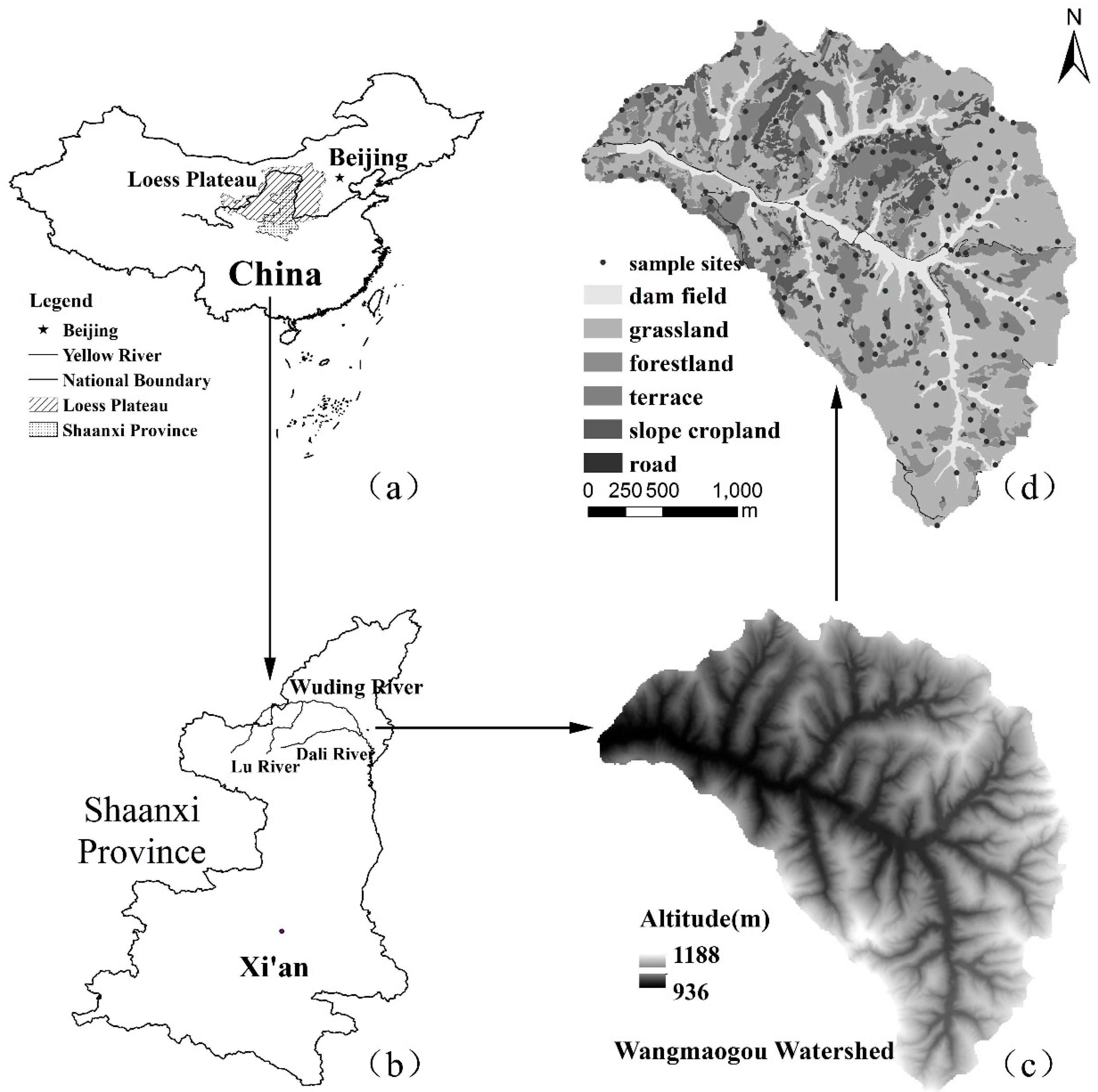
2.1. Study Area

The study area is located in the Wangmaogou Basin (110°20′26″–110°22′46″ E, 37°34′13″–37°36′03″ N) of the Loess Plateau, and in the Wuding River Basin 5 km north of Suide County, Shaanxi Province, China (Figure 1). The area of the watershed is 5.97 km², the altitude is between 936 m and 1188 m, and the annual average temperature is 10.2 °C. The average annual precipitation in this area is about 513 mm, which is unevenly distributed during the year, and the rainfall from July to September makes up 60% of the entire year. The soil is dominated by loessal soil. The loess has developed vertical joints and uniform particles, but the clay content is low and the cementation is weak, which can easily cause serious soil erosion when affected by rainfall during the flood season. Since 1950, many water and soil conservation measures have been implemented in the Wangmaogou Basin, and therefore this basin can be used as a typical watershed for water and soil conservation research. The main types of land use in the basin are sloping cropland (22.32%), forestland (9.15%), grassland (36.51%), terrace (25.78%), and check dam (6.24%).

2.2. Methods

2.2.1. Soil Sample Collection and Determination Methods

Soil samples were collected from July to August in 2014 by using a drill with a diameter of 6.9 cm. The sampling depth was 100 cm, and soil samples from each soil layer were collected at depths of 0–20 cm, 20–40 cm, 40–60 cm, 60–80 cm, and 80–100 cm. The average interval for each sample point was 100 m. The numbers of soil samples collected under different land use patterns were 18 (terrace), 114 (grassland), 48 (forestland), 20 (sloping cropland), and 16 (check dam). In the process of collecting soil samples, the altitude, gradient, slope aspect, vegetation type, and coverage of sampling points have also been recorded. The analysis of SAP used a fully automated intermittent analyzer. The soil bulk density was measured with a ring knife. A total of 15 soil profiles were taken in the sloping cropland, forestland, grassland, terrace, and check dam, which were 60 cm deep, sampled at 20 cm intervals, and brought back to the laboratory oven at 105 °C. The soil bulk density was measured after 10 h of drying. Soil thicknesses of 0–20 cm, 20–40 cm, 40–60 cm, 60–80 cm, and 80–100 cm are indicated by A1, A2, A3, A4, and A5, respectively.

2.2.2. Data Analysis and Processing Methods

The descriptive statistical analysis is performed by SPSS (20.0) software, the semi-variance function is calculated by GS + (7.0), and the spatial distribution map is produced by ArcGIS (10.1).

The semi-variance function is a key function for studying the spatial variability of soil in geostatistics. Its theoretical model can be applied to analyze the randomness and structure of the spatial variability of SAP. It is expressed by Equation (1), as follows [19]:

$$\gamma \left(h\right)=\frac{1}{2N\left(h\right)}{\displaystyle \sum }_{i=1}^{N\left(h\right)}{\left[z\left(x_i\right)-z\left(x_i+h\right)\right]}^2$$

(1)

In Equation (1), γ(h) is the semi-variance function; z(x_i) − z(x_i + h) is the measured value of two observation points with interval h; N(h) is the pair number of all observation points in steps of h. The semi-variance function diagram is usually obtained by plotting γ(h) in line with h. Usually, the value of the semi-variance function increases with the distance from the sample points, and increases to a substantially stable constant within a certain range of variation, namely the base value. A reasonable theoretical model can be obtained by fitting the semi-variance function according to the determination coefficient R2 and the residual RSS.

The calculation of SAP reserves uses the calculation formula of soil organic carbon reserves [20]:

$$C_i=d_i\times {\rho }_i\times O_i/100$$

(2)

$$W_i=A_i\times C_i$$

(3)

In the formula, i is different levels of soil; C is SAP density (g/m²); d is the thickness of soil (cm); p is soil bulk density (g/cm³), O is SAP content (mg/kg); A is the area occupied by each type; and W is SAP reserves.

3. Results

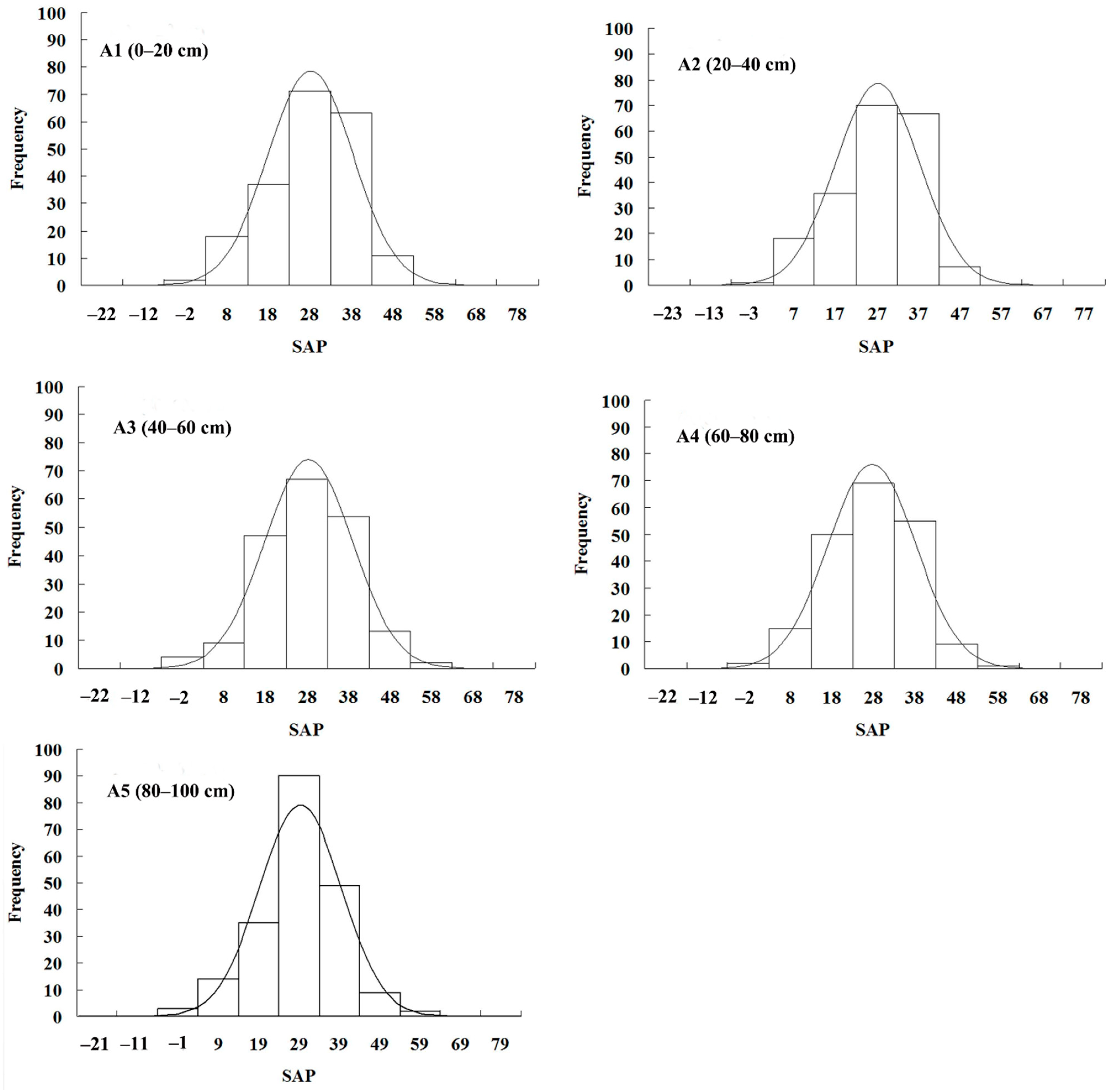
3.1. Statistical Characteristics of SAP

As can be seen from

Table 1. Statistical characteristics of SAP at different depths (mg/kg).

Layer Depth (cm)	Mean Value	Standard Deviation	Min.	Max.	Skewness	Kurtosis	K-S (p)	CV (%)
A1	28.19	10.27	1.14	50.4	−0.39	−0.19	0.52	36
A2	27.26	10.12	1.17	50.72	−0.45	−0.26	0.35	37
A3	28.4	10.56	0.7	54.57	−0.15	−0.03	0.48	37
A4	27.66	10.54	0.52	57.15	−0.24	−0.05	0.87	38
A5	29.37	10.21	2.62	59.25	−0.15	0.43	0.71	35

, the available phosphorus content in different soil depths was tested by ANOVA, and there is a significant difference in SAP at different soil depths (p < 0.01), which is huge between the minimum and maximum values, close to 50 times. The maximum average value is in layer A5, and the minimum in layer A2, which are 29.37 mg/kg and 27.26 mg/kg, respectively. The variations of available phosphorus are from 35% in the A5 layer to 38% in the A4 layer. According to the classification system proposed by Nielson and Bouma [21] (pp. 170–175), the weak variation CV is ≤ 10%; the moderate variation is 10% < CV < 100%; and the strong variation CV is ≥100%. Consequently, the variation coefficients of available phosphorus in all five soil layers are moderately variable.

For geostatistical analysis, since the Kriging method has the highest prediction accuracy for normal distribution data, it is indispensable to test whether the data set of SAP satisfies normal distribution before conducting geostatistical analysis. From the K-S test and the skewness and kurtosis, it can be discovered that the SAPs in the five soil layers all obey the normal distribution (p > 0.05) and meet the requirements of the next-step analysis. The normal distribution curve is shown in Figure 2.

3.2. Changes of SAP and Bulk Density with Different Land Uses

Dual-factor ANOVA has shown that land use and soil depth significantly affect SAP content (p < 0.01).

Table 2. Mean values and bulk density of SAP under different land uses.

Layer Depth (cm)	Terrace		Grassland		Forestland		Sloping Cropland		Check Dam
	SAP	Bulk Density	SAP	Bulk Density	SAP	Bulk Density	SAP	Bulk Density	SAP	Bulk Density
	(mg/kg)	(g/cm3)	(mg/kg)	(g/cm3)	(mg/kg)	(g/cm3)	(mg/kg)	(g/cm3)	(mg/kg)	(g/cm3)
A1	30.53	1.28	28.95	1.26	26.52	1.27	28.51	1.29	30.7	1.37
A2	28.6	1.35	28.33	1.35	24.85	1.28	26.83	1.36	27.12	1.17
A3	29.24	1.34	29.19	1.4	26.87	1.32	25.3	1.32	27.04	1.33
A4	28.15	-	29.5	-	24.59	-	26.12	-	24.94	-
A5	29.06	-	29.97	-	26.73	-	25.36	-	25.09	-
Mean Value	29.11	1.32	29.19	1.34	25.84	1.29	26.42	1.32	26.98	1.29

contains the average SAP content and bulk density under different land uses, from which the average SAP content of the five land types in a descending order is: grassland > terrace > check dam > sloping cropland > forestland. The SAP content in the terrace and dam of layer A1 is dramatically higher than other lands. The soil bulk density under different land uses shows that: grassland > terrace > sloping cropland > forestland = dam.

3.3. Relationship between SAP Content and Topographic Factors

Table 3. Average SAP content in different land uses under topographic factors.

Terrain Factors		Gradient (°)						Altitude (m)				Slope Aspect
		0–3	3–8	8–15	15–25	25–35	>35	≤1000	1000–1050	1050–1100	>1100	Sunny Slope	Shady Slope
Check Dam	A1	26.26	-	-	-	-	-	29.78	31.49	-	-	30.7	-
	A2	23.91	-	-	-	-	-	29.5	25.07	-	-	27.12	-
	A3	29.5	-	-	-	-	-	27.42	26.72	-	-	27.04	-
	A4	23.96	-	-	-	-	-	25.57	24.4	-	-	24.94	-
	A5	28.8	-	-	-	-	-	28.06	22.56	-	-	25.09	-
Terrace	A1	29.66	-	-	-	-	-	32.53	33.91	28.28	9.66	28.6	30.35
	A2	27.57	-	-	-	-	-	32.72	30.86	25.62	11.42	27.62	27.54
	A3	28.31	-	-	-	-	-	30.71	32.26	27.15	9.57	30.69	26.76
	A4	27.91	-	-	-	-	-	31.55	29.02	28.67	14.68	27.61	28.1
	A5	29.49	-	-	-	-	-	29.18	31.33	31.82	12.21	29.24	29.66
Grassland	A1	-	27.59	30.86	27.42	27.48	31.63	38	28.8	29.7	26.84	28.88	29.2
	A2	-	31.63	29.12	27.26	25.18	31.53	38.05	29.6	27.18	26.45	27.33	28.94
	A3	-	29.73	33.05	25.85	29.98	29.56	35.46	29.13	29.99	26.5	29.32	28.99
	A4	-	25.06	31.82	26.17	28.59	31.12	34.86	29.03	30.99	24.16	29.05	28.85
	A5	-	29.69	33.04	29.89	27.43	32.65	37.5	30.61	30.11	29.04	30.3	30.36
Forestland	A1	25.28	22.28	22.31	28.9	19.89	27.65	27.94	26.39	28.38	22.43	25.8	24.86
	A2	6.53	19.02	22	30.19	22.69	27.69	31.71	25.66	23.44	23.57	26.03	23.14
	A3	0.7	25.33	20.06	36.15	19.06	31.25	27.38	28.78	24.67	27.22	27.64	26.6
	A4	26.69	21.79	20.27	29.26	21.76	27.43	24.37	25.34	25.24	25.13	26.6	22.72
	A5	16.37	31.69	21.49	34.16	28.48	30.08	35.83	26.41	27.09	30.07	31.69	23.69
Sloping Cropland	A1	-	33.1	27.2	28.05	21.34	27.06	31.14	21.18	22.72	30.95	25.51	25.94
	A2	-	26.18	27.45	28.29	26.04	27.56	30.59	23.32	27.84	26.06	27.89	26.68
	A3	-	31.87	23.82	27.44	23.37	19.28	26.52	20.35	27.86	30.79	26.5	24.53
	A4	-	24.22	29.33	30.58	21.48	30.69	30.99	19.69	30.13	24.5	22.31	28.44
	A5	-	29.72	31.18	26.83	21.32	21.06	24.35	22.44	26.3	31.62	22.66	25.98

shows the average SAP content of different land uses under topographic factors. According to the actual situation in the study area, the altitude is composed of 4 levels, ≤1000 m, 1000–1050 m, 1050–1100 m, and >1100 m; the slope consists of 6 levels, flat slope (0–3°), slight slope (3–8°), slope (8–15°), slightly steep slope (15–25°), steep slope (25–35°), and extremely steep slope (>35°); and, the slope aspect is divided into shady slope and sunny slope [22]. The effect of topographic factors on SAP content is considerably different under different land use conditions. In light of the ANOVA analysis, there is a substantial correlation between altitude and SAP content in terrace, grassland, and sloping cropland (p < 0.01), but the correlation between altitude and SAP content in dam and forestland is not evident (p > 0.05). The relationship between gradient and SAP content in grassland, forestland, and sloping cropland is striking (p < 0.01); however, the slope aspect only has a distinct correlation with the SAP content in forestland (p < 0.05), but not in other land uses (p > 0.05).

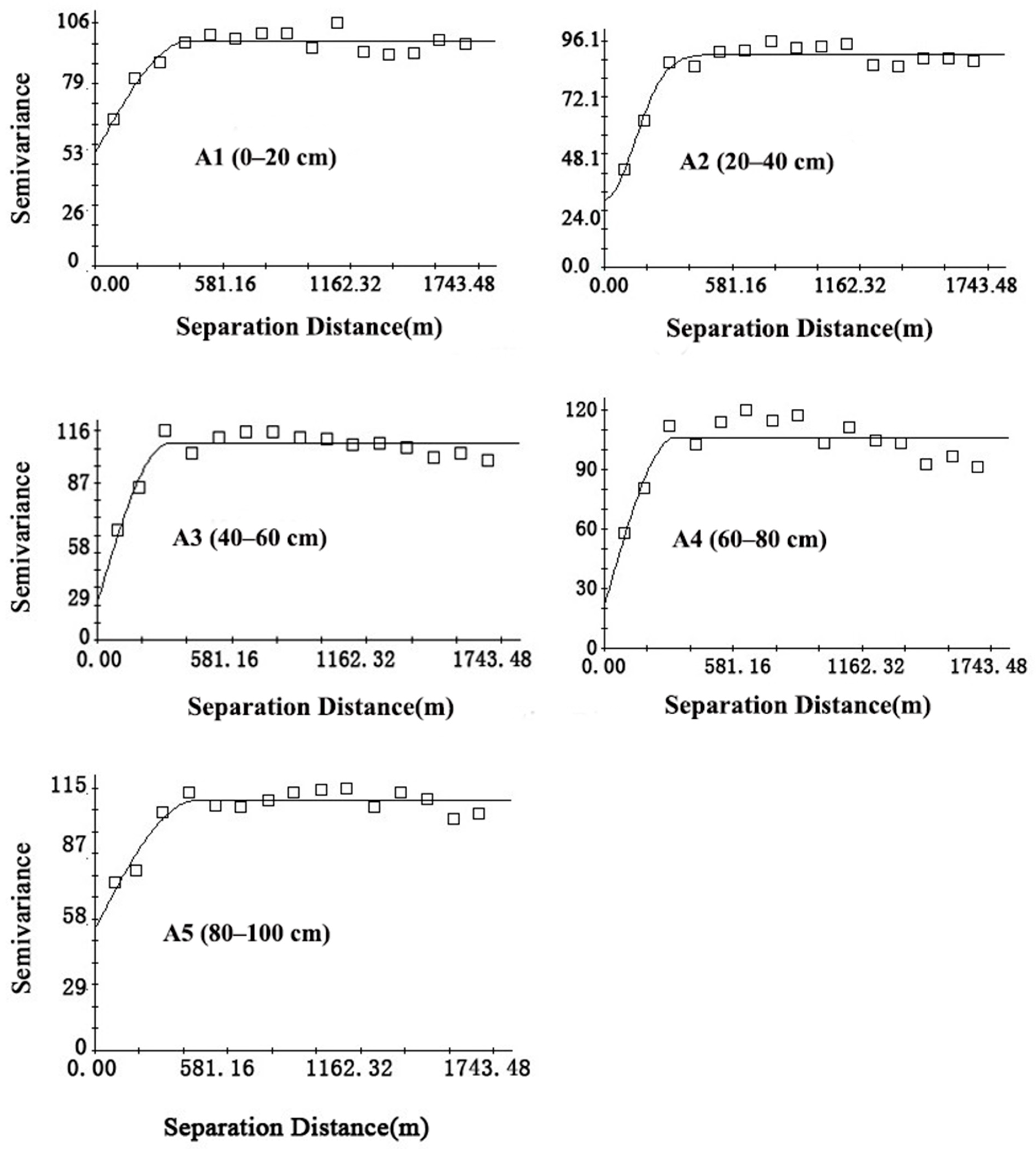
3.4. Geostatistics Analysis of SAP

Table 4. Geostatistical parameters of SAP at different depths.

Layer Depth	C0	C0 + C	Nugget Coefficient	Variation Amplitude	Model	R2	Residual
			GD (%)	(m)			RSS
A1	49	98	50	424	Spherical	0.861	205
A2	28.7	90.35	68	194	Gaussian	0.941	170
A3	20.8	108.8	81	308	Spherical	0.859	410
A4	21.1	106.2	80	322	Spherical	0.71	1068
A5	53.5	110	51	493	Spherical	0.867	285

shows the geostatistical parameters of SAP at different soil depths. The model with the highest fitting degree (R2) and the smallest residual sum of squares (RSS) is selected as the optimal model (Figure 3). Under the five soil layers, the optimal models of SAP are all linear models, whose determination coefficients are 0.861, 0.941, 0.859, 0.71, and 0.867, and the RSS is also smaller, indicating that the model has high fitting accuracy and can well reflect the spatial structure characteristics of SAP in the study area. The nugget coefficient represents the degree of spatial correlation of system variables. When the ratio is <25%, the system has a strong spatial correlation; 25–75%, a medium spatial correlation; and >75%, a weak spatial correlation. The nugget coefficients of SAP of all layers are relatively large, accounting for 50–81%, indicating that the spatial variability of SAP is mainly attributed to structural and random factors. Structural factors such as climate, parent material, topography, soil type, and other natural factors can lead to strong spatial correlation of soil nutrients; while random factors such as fertilization, farming measures, cropping systems, and other human activities undermine spatial correlation of SAP, thus developing in the direction of homogenization. The variations of the five soil depths (194–493 m) are larger than the grid sampling interval of 100 m used in this research and satisfy the spatial analysis requirements.

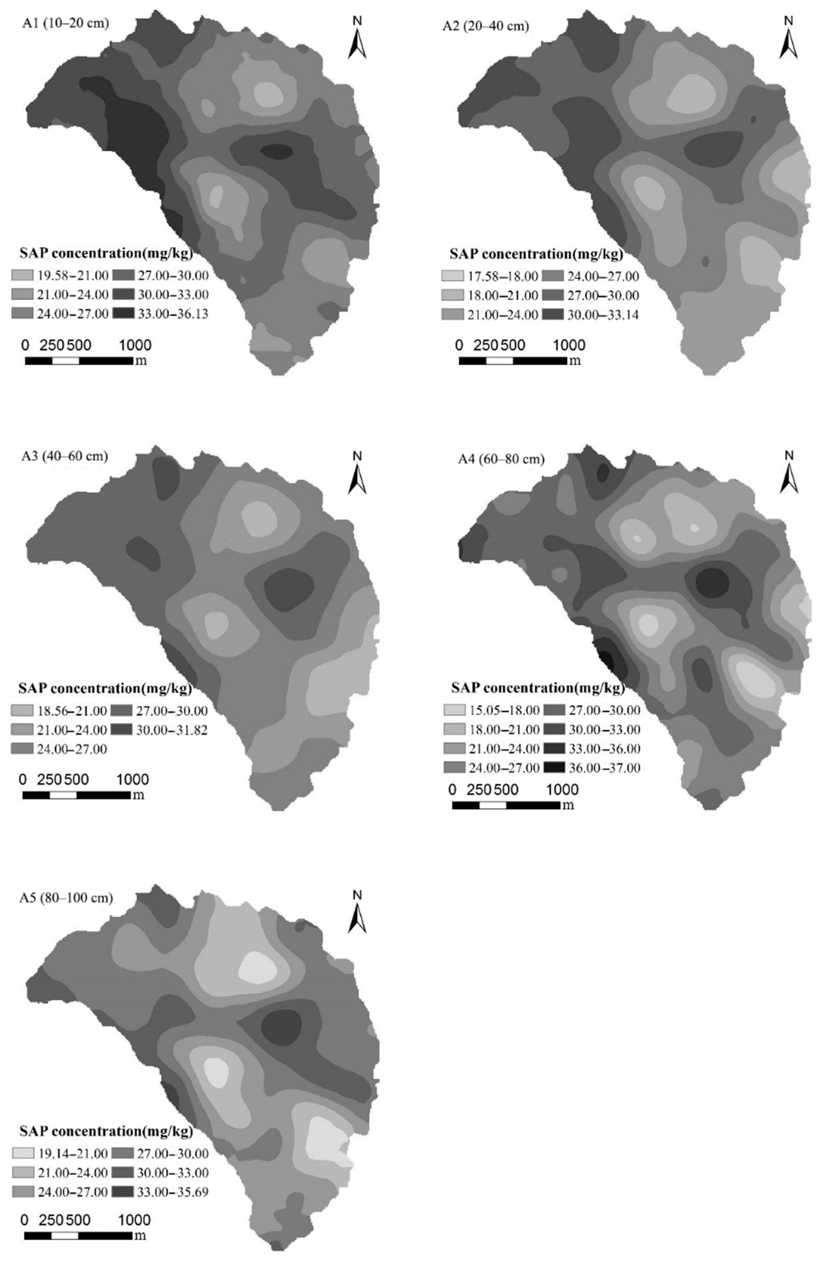
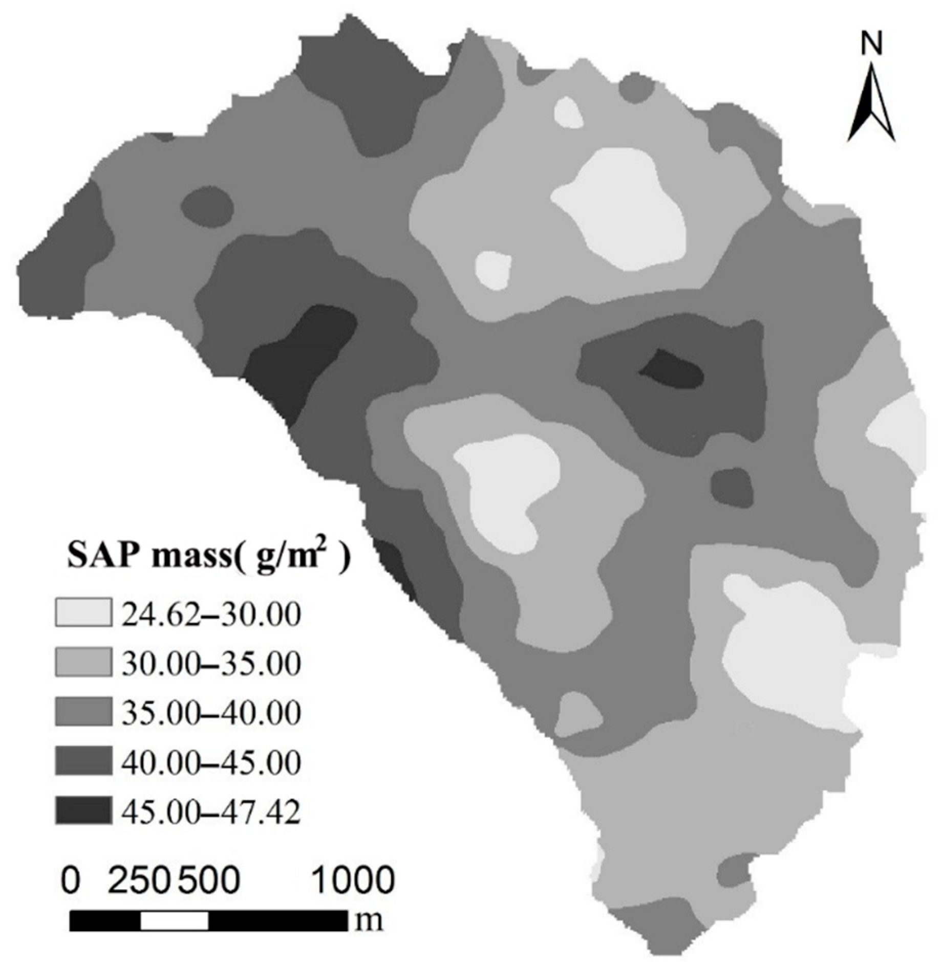
3.5. Spatial Distribution of SAP

Kriging interpolation is applied to the SAP values at five sampling depths, plotting the spatial distribution of SAP in the five soil layers of Wangmaogou Basin (Figure 4). It can be seen from the figure that the SAP in the five soil layers shows a patchy distribution. As the depth increases, the available phosphorus content gradually decreases, and so does the change range of the available phosphorus. The SAP content in layer A1 is the highest and in layer A5 is the lowest. The highest SAP is generally at the intersection of rivers, such as grassland and dam land. Hence, the spatial distribution characteristics of SAP are closely related to land use types.

3.6. SAP Density and Reserves under Different Land Uses

According to Equations (2) and (3), the SAP density and reserves under different land uses in Wangmaogou Basin are calculated. According to the SAP density under different land uses (

Table 5. SAP density of layers under different land uses.

Layer Depth (cm)	Terrace		Grassland		Forestland		Sloping Cropland		Check Dam
	SAP	CV	SAP	CV	SAP	CV	SAP	CV	SAP	CV
	(g/m2)	(%)	(g/m2)	(%)	(g/m2)	(%)	(g/m2)	(%)	(g/m2)	(%)
A1	7.91	9.51	7.08	3.77	6.44	5.52	7.16	8.47	7.77	7.02
A2	7.63	9.96	7.21	3.98	6	7.24	7.11	8.24	6.01	6.81
A3	7.97	8.89	7.2	4.27	6.43	8.17	6.6	8.6	7.07	6.49
A4	7.51	8.71	7.67	3.98	6.3	6.02	6.86	9.95	6.68	6.31
A5	7.98	8.83	7.95	3.56	6.63	7.16	6.65	8.6	6.67	7.32
0–100 cm	39	8.63	37.12	3.51	31.81	6.29	34.37	8.31	34.19	5.78

and Figure 5), its maximum and minimum values appear in the terrace and the forestland. The SAP of layer A1 in different land uses varies greatly, which in descending order is: terrace > dam > sloping cropland > grassland > forestland. Shown by the variation coefficient of SAP density, the variations of SAP under five soil depths are weak, and the highest and lowest are discovered in terrace and grassland, respectively. Under different land uses, the SAP reserves at a depth of 0–100 cm are as follows: grassland (123.64 t) > sloping cropland (20.21 t) > check dam (17.31 t) > terrace (11.56 t) > forestland (9.80 t). The total SAP reserves of 0–100 cm layer in the Wangmaogou Basin are 182.51 t.

4. Discussion

The average SAP content in grassland is higher than in the other four land types, whereas that in sloping cropland is apparently lower than the other four land types. This indicates that the sloping cropland will increase after being converted into grassland, terrace, or check dam, which bears a resemblance to the studies of Xin [23] and Liu et al. [24], who found that the implementation of the ecological construction of the Loess Plateau effectively enhanced the role of soil organic carbon sinks, making the basin a repository for carbon and phosphorus. In addition, the SAP content in layer A1 of check dam is evidently higher than that of the other land types, and the content of organic matter and clay in the silt intercepted by check dam is usually higher than that of the source soil [25]. The soil clay content under the five types of lands is very low (the maximum value is less than 9%), and there is no significant difference (p > 0.05) in the grain size under different land types. Because the dam is mainly distributed in the lower channels in the study area, fine soil particles on the slope are carried by rainfall and runoff and deposited on the dam. With a large specific surface area and charge density, the soil clay has a strong adsorption capacity for soil nutrients and can form relatively stable organic–inorganic composites with macromolecular organic substances (especially humus). These composites can form a more stable aggregate structure which has the effect of enhancing the accumulation of soil nutrients [26], and therefore the STP content of the dam is relatively high. This research result is consistent with that of Liu et al. [24], who gathered that the dam construction could intercept large amounts of sediment and phosphorus. In consequence, the construction of check dam in the Loess Plateau can significantly increase soil phosphorus content and increase soil fertility.

The variation of SAP is closely related to the complex terrain factors [27]. Changes in topography such as gradient, slope aspect, and altitude can lead to changes in an array of biological and abiotic activities [28], such as soil water content, microbial activity, water–heat balance, plant growth, and the amount of litters, thereby affecting SAP content. Previous studies have detected that there is an immense correlation between SAP and gradient, as well as a dramatic negative correlation between SAP and altitude. However, Wang et al. [29] found that soil nutrients could not be affected by the slope aspect. This article has discovered that the effects of topographic factors on SAP are different under different land use conditions, for which the reason is: the ecological construction measures in the Loess Plateau have caused a series of changes in vegetation coverage, soil properties, and water–heat balance, which is closely related to SAP content, thus reducing the influence of topographic factors on SAP and resulting in the different impacts of topography on SAP content in different land types.

5. Conclusions

There are prominent differences in SAP at different soil depths and under various land uses. The average contents of SAP under five soil layers of A1, A2, A3, A4, and A5 are 28.19 mg/kg, 27.26 mg/kg, 28.40 mg/kg, 27.66 mg/kg, and 29.37 mg/kg, and the spatial variability of SAP under the five soil layers is moderate. The average SAP content in the five land types in descending order is as follows: grassland > terrace > check dam > sloping cropland > forestland. The SAP content in terrace and dam of layer A1 are significantly higher than that of other land uses. In summary, converting the sloping cropland to grassland, terrace, or dam can raise SAP content.

The variation of SAP is closely related to topographic factors. Under different types of land use, the influencing factors are different: the altitude is significantly related to the SAP content in terrace, grassland, and sloping cropland (p < 0.01); the gradient is significantly related to the SAP content in grassland, forestland, and sloping cropland (p < 0.01); while the slope aspect only affects the SAP content in forestland (p < 0.05).

The spatial distribution of SAP under the five soil layers in Wangmaogou Basin is patchy. With the increase of depth, the available phosphorus content gradually decreases, and so does its change range. The highest values of SAP spatial distribution in the study area usually occur in grassland and dam. At the depth of five soil layers, the maximum and minimum values of SAP density appear in terrace and forestland, respectively. The SAP density varies significantly among different land types in layer A1, which in a descending order is: terrace > check dam > sloping cropland > grassland > forestland. The total SAP reserves of the 0–100 cm layer in the Wangmaogou Basin are 182.51 t.

References

1. Bureau, M.F.; Mederski, H.J.; Evans, C.E. The effect of phosphatic fertilizer material and soil phosphorus level on the yield and phosphorus uptake of soybeans. Agron. J. 1953, 45, 150–154. [Google Scholar] [CrossRef]
2. Mehnaz, K.R.; Keitel, C.; Dijkstra, F.A. Phosphorus availability and plants alter soil nitrogen retention and loss. Sci. Total Environ. 2019, 671, 786–794. [Google Scholar] [CrossRef] [PubMed]
3. Mao, R.; Zhang, X.-H.; Li, S.-Y.; Song, C.-C. Long-term phosphorus addition enhances the biodegradability of dissolved organic carbon in a nitrogen-limited temperate freshwater wetland. Sci. Total Environ. 2017, 605, 332–336. [Google Scholar] [CrossRef]
4. Gaind, S.; Pandey, A.K. Microbial biomass, P-nutrition, and enzymatic activities of wheat soil in response to phosphorus enriched organic and inorganic manures. J. Environ. Sci. Health Part B 2006, 41, 177–187. [Google Scholar] [CrossRef] [PubMed]
5. Meinikmann, K.; Hupfer, M.; Lewandowski, J. Phosphorus in groundwater discharge—A potential source for lake eutrophication. J. Hydrol. 2015, 524, 214–226. [Google Scholar] [CrossRef]
6. Daniel, T.C.; Sharpley, A.N.; Lemunyon, J.L. Agricultural phosphorus and eutrophication: A symposium overview. J. Environ. Qual. 1999, 27, 251–257. [Google Scholar] [CrossRef] [Green Version]
7. Cheng, S.D.; Li, Z.B.; Li, P.; Li, J. Experimental study on dynamic process of soil water-nutrient loss on slope with different pattern of grass. J. Soil Water Conserv. 2014, 28, 58–61, (In Chinese with English abstract). [Google Scholar]
8. Yan, P.; Shen, C.; Fan, L.; Li, X.; Zhang, L.; Zhang, L.; Han, W. Tea planting affects soil acidification and nitrogen and phosphorus distribution in soil. Agric. Ecosyst. Environ. 2018, 254, 20–25. [Google Scholar] [CrossRef]
9. Junior, R.V.; Varandas, S.G.P.; Fernandes, L.S.; Pacheco, F.A.L. Groundwater quality in rural watersheds with environmental land use conflicts. Sci. Total Environ. 2014, 493, 812–827. [Google Scholar] [CrossRef]
10. Ordóñez-Fernández, R.; Rodríguez-Lizana, A.; Espejo-Pérez, A.J.; González-Fernández, P.; Saavedra, M.M. Soil and available phosphorus losses in ecological olive groves. Eur. J. Agron. 2007, 27, 144–153. [Google Scholar] [CrossRef]
11. Valera, C.A.; Valle, R.F., Jr.; Varandas, S.; Fernandes, L.; Pacheco, F. The role of environmental land use conflicts in soil fertility: A study on the Uberaba River basin, Brazil. Sci. Total Environ. 2016, 562, 463–473. [Google Scholar] [CrossRef]
12. Zhang, K.; Li, S.; Peng, W.; Yu, B. Erodibility of agricultural soils on the Loess Plateau of China. Soil Tillage Res. 2004, 76, 157–165. [Google Scholar] [CrossRef] [Green Version]
13. Fu, B.; Liu, Y.; Lü, Y.; He, C.; Zeng, Y.; Wu, B. Assessing the soil erosion control service of ecosystems change in the Loess Plateau of China. Ecol. Complex. 2011, 8, 284–293. [Google Scholar] [CrossRef]
14. Feng, X.; Fu, B.; Piao, S.; Wang, S.; Ciais, P.; Zeng, Z.; Lü, Y.; Zeng, Y.; Li, Y.; Jiang, X.; et al. Revegetation in China’s Loess Plateau is approaching sustainable water resource limits. Nat. Clim. Chang. 2016, 6, 1019–1022. [Google Scholar] [CrossRef]
15. Ma, H.B.; Li, J.J.; He, X.Z.; Liu, X.Y.; Wang, F.G. The status and sediment reduction effects of level terrace in the Loess Plateau. Yellow River 2015, 37, 89–93, (In Chinese with English abstract). [Google Scholar]
16. Qiu, L.P. Change of Soil Quality and Its Regulation in Re-Vegetation Ecosystem of the Loess Plateau; Northwest A.&F. University: Xianyang, China, 2007. [Google Scholar]
17. Fang, X.; Xue, Z.; Li, B.; An, S. Soil organic carbon distribution in relation to land use and its storage in a small watershed of the Loess Plateau, China. CATENA 2012, 88, 6–13. [Google Scholar] [CrossRef]
18. Deng, L.; Wang, G.-L.; Liu, G.-B.; Shangguan, Z.-P. Effects of age and land-use changes on soil carbon and nitrogen sequestrations following cropland abandonment on the Loess Plateau, China. Ecol. Eng. 2016, 90, 105–112. [Google Scholar] [CrossRef]
19. Liu, Q.; Xia, J.; Xie, W. Application of semi-variogram and Moran’s I to spatial distribution of trace elements in soil: A case study in Shouguang County. Geomat. Inf. Sci. Wuhan Univ. 2011, 36, 1129–1133. [Google Scholar]
20. Xu, G.C.; Li, Z.B.; Li, P.; Liu, X.J.; Gao, H.D. Study on TN spatial variability of Yingwugou small watershed in Dan River. J. Soil Water Conserv. 2011, 25, 59–63, (In Chinese with English abstract). [Google Scholar]
21. Nielsen, D.R.; Bouma, J. Soil spatial variability. In Proceedings of the Workshop of the ISSS and the SSSA, Las Vegas, NV, USA, 30 November—1 December 1984; pp. 170–175. [Google Scholar]
22. Zhao, B.; Li, Z.; Li, P.; Xu, G.; Gao, H.; Cheng, Y.; Chang, E.; Yuan, S.; Zhang, Y.; Feng, Z. Spatial distribution of soil organic carbon and its influencing factors under the condition of ecological construction in a hilly-gully watershed of the Loess Plateau, China. Geoderma 2017, 296, 10–17. [Google Scholar] [CrossRef]
23. Xin, Z.; Qin, Y.; Yu, X. Spatial variability in soil organic carbon and its influencing factors in a hilly watershed of the Loess Plateau, China. Catena 2016, 137, 660–669. [Google Scholar] [CrossRef]
24. Liu, C.; Li, Z.; Dong, Y.; Nie, X.; Liu, L.; Xiao, H.; Zeng, G. Do land use change and check-dam construction affect a real estimate of soil carbon and nitrogen stocks on the Loess Plateau of China? Ecol. Eng. 2017, 101, 220–226. [Google Scholar] [CrossRef]
25. Sharpley, A.N. The selection erosion of plant nutrients in Runoff. Soil Sci. Soc. Am. J. 1985, 49, 1527–1534. [Google Scholar] [CrossRef]
26. Li, X.Y. Contents and Characteristic of Different from Organic Carbon and Nitrogen in Rhizosphere; Northwest A.&F. University: Xianyang, China, 2011. [Google Scholar]
27. Liu, D.; Wang, Z.; Zhang, B.; Song, K.; Li, X.; Li, J.; Li, F.; Duan, H. Spatial distribution of soil organic carbon and analysis of related factors in croplands of the black soil region, Northeast China. Agric. Ecosyst. Environ. 2006, 113, 73–81. [Google Scholar] [CrossRef]
28. Wang, H.Q.; Hall, C.A.S.; Cornell, J.D.; Hall, M.H.P. Spatial dependence and the relationship of soil organic carbon and soil moisture in the Luquillo, Experimental Forest, Puerto Rico. Landsc. Ecol. 2002, 17, 671–684. [Google Scholar] [CrossRef]
29. Wang, Y.-Q.; Zhang, X.-C.; Zhang, J.-L.; Li, S.-J. Spatial variability of soil organic carbon in a watershed on the Loess Plateau. Pedosphere 2009, 19, 486–495. [Google Scholar] [CrossRef]
Figure 1. Location map of the Loess Plateau in China (a), Location map of Wuding River in Shaanxi Province (b), The Digital Elevation Model of the Wangmaogou watershed (c), Land use types (d), The sampling point distribution (d) (The direction of the arrow is the layout of the study area from large to small in China).
Sustainability 13 12572 g001
Figure 2. Normal distribution curve of soil available phosphorus in 0~20 cm layer (A1); Normal distribution curve of soil available phosphorus in 20~40 cm layer (A2); Normal distribution curve of soil available phosphorus in 40~60 cm layer (A3); Normal distribution curve of soil available phosphorus in 60~80 cm layer (A4); Normal distribution curve of soil available phosphorus in 80~100 cm layer (A5).
Sustainability 13 12572 g002
Figure 3. Semi variance function theoretical model of available phosphorus in 0~20 cm soil layer (A1); Semi variance function theoretical model of available phosphorus in 20~40 cm soil layer (A2); Semi variance function theoretical model of available phosphorus in 40~60 cm soil layer (A3); Semi variance function theoretical model of available phosphorus in 60~80 cm soil layer (A4); Semi variance function theoretical model of available phosphorus in 80~100 cm soil layer (A5).
Sustainability 13 12572 g003
Figure 4. Spatial interpolation distribution of available phosphorus content in 0~20 cm soil layer (A1); Spatial interpolation distribution of available phosphorus content in 20~40 cm soil layer (A2); Spatial interpolation distribution of available phosphorus content in 40~60 cm soil layer (A3); Spatial interpolation distribution of available phosphorus content in 60~80 cm soil layer (A4); Spatial interpolation distribution of available phosphorus content in 80~100 cm soil layer (A5).
Sustainability 13 12572 g004
Figure 5. SAP density distribution in 0–100 cm soil in Wangmaogou Basin.
Sustainability 13 12572 g005