A Systematic Methodology for Design of Sustainable Urban Neighborhood Energy Infrastructure

Abstract

The growing share of global energy consumption by cities (currently over 65%) raises the requirements for a systematic holistic approach for designing urban energy infrastructure in order to ensure its sustainability. A literature review of state-of-the-art modeling of urban energy infrastructure design emphasized the incomprehensive sustainability of the performed evaluations, as they accounted for several aspects of sustainability but missed others. Omitting important aspects can have significant implications which can put the sustainability of the energy infrastructure at risk. In this study, we attempted to develop a comprehensive model for designing sustainable energy infrastructure for urban districts, which accounts for the four aspects of sustainability: social, technical, environmental, and economic. The model is based on a four-step methodology: district characterization, a technological survey for distributed generation and energy storage, selecting suitable technologies according to social and technical criteria, and simulations of different energy infrastructure configurations to find the most suitable configurations basing on economic and environmental criteria. The research includes a case study in which the model was implemented for the Technion campus in Haifa. The developed model proved to be a comprehensive, efficient, and versatile tool for designing urban energy infrastructure.

1. Introduction

Global urbanization makes cities the largest energy consumer of worldwide. In 2013 cities were responsible for 64% of global energy consumption. As a result, cities produced about 70% of global greenhouse gas (GHG) emissions [1]. These shares are projected to grow even larger, as the UN project 60% of the world population will live in cities by 2030 and 68% will live in cities by 2050 [2]. This makes urban energy infrastructure the main concern for the energy sector. Furthermore, the need for sustainable urban energy infrastructures has been emphasized in order to raise their ability to remain operational for long durations.

Sustainability of energy infrastructure has various aspects, each having a significant impact on the its durability. These include environmental, economic, social, and technical aspects. Evaluating the sustainability of energy infrastructures according to these aspects is based on qualitative and quantitative evaluations of several pertinent criteria. The environmental criteria traditionally employed is concerned with sustainability of energy infrastructures and aimed at evaluating their environmental impact. These include the amounts of GHG emissions and air pollution associated with the infrastructure, the amount of land used by the infrastructure equipment, and the noise levels from energy systems operation [3,4,5,6,7,8,9,10]. Economic criteria used in practice are used to evaluate costs and benefits associated with the energy infrastructure life cycle. The economic indicators normally employed, include investment costs, operation, and maintenance costs, revenues, and the internal rate of return (IRR). Investment costs include all initial costs associated with the energy infrastructure, including equipment purchasing and installation. Furthermore, revenues include income from selling energy, and other co-benefits associated with the infrastructure. These indicators are often used to evaluate the infrastructure economic aspect using different criteria, including the net present value (NPV), life cycle costs (LCC), and levelized cost of energy (LCOE) [3,4,5,6,7,8,9,10,11]. Technical criteria used in previous projects aim at evaluating the equipment used by the infrastructure. Technical indicators include reliability, efficiency, safety, stability, life span, commercial maturity, and capacity factor of the equipment, as well as the availability of needed resources in the infrastructure area [4,5,6,10,11]. Social criteria are designed to evaluate the impact of the infrastructure on the residents’ well-being, which is their perception of being healthy and happy [12]. Social indicators include indoor comfort, job creation by the infrastructure, its accessibility for residents, the impact on the public health, and the infrastructure’s social acceptability [3,4,5,6,9,10].

The existing literature presents projects for modeling urban energy infrastructure design. Pica et al. (2013) presented a four-step methodology for planning distributed energy generation in urban districts, based on the concept of smart microgrids. Furthermore, the sustainability evaluation of the energy infrastructure in their methodology includes only economic and technical aspects [11]. Ristimäki et al. (2013) presented a model for designing residential district energy systems, which is based on a combined LCC and life cycle assessment (LCA) decision-making method. As such, their model accounts for economic and environmental aspects only in the sustainability evaluation of the energy infrastructure [7]. Similarly, Alkhalidi et al. (2018) presented a model for designing a new sustainable city accounting for economic and environmental aspects only [8]. Becchio et al. (2018) presented a method for design of net-zero energy district based on a cost-benefit analysis (CBA). As such, the sustainability evaluation in their method included only fiscally quantifiable aspects [9]. Lastly, Amado et al. (2017) presented a model for design of net-zero cities based on technical evaluations only [13]. One shortcoming of these models is their incomprehensive evaluation of the sustainability of the infrastructure, wherein each model accounts for several sustainability aspects but misses others. This incomprehensive evaluation can risk the sustainability of the infrastructure, as omission of aspects can have far-reaching implications. For example, omitting social aspects of the infrastructure can raise resistance from residents which can result in ceasing the operation of the infrastructure [5]. As such, there arises a need for a comprehensive model for the design of sustainable urban energy infrastructures, having environmental, economic, technical, and social aspects all together. The need for a comprehensive evaluation of the sustainability of the energy infrastructure was further emphasized by [14,15].

As such, the goal of this research is building and testing a comprehensive model for design of urban energy infrastructure which accounts for all different aspects of sustainability, including technical, social, economic, and environmental aspects.

In short, the main contributions of this research are:

• The development of a systematic model for designing urban energy infrastructure which considers all four sustainability aspects.
• Proposing a combined qualitative and quantitative evaluation of the sustainability of the energy infrastructure.
• Proposing a qualitative evaluation of the technical and social aspects of the energy infrastructure which is based on subjective assessment, in order to increase social engagement and to increase the acceptability of the infrastructure by the population.

The rest of the paper is organized as follows: following the introduction, Section 2 presents the model developed in this research. A case study for implementing the model is presented in Section 3. Section 4 presents a discussion of the results, and finally, the important conclusions of this research are presented in Section 5.

2. Model

2.1. Model Overview

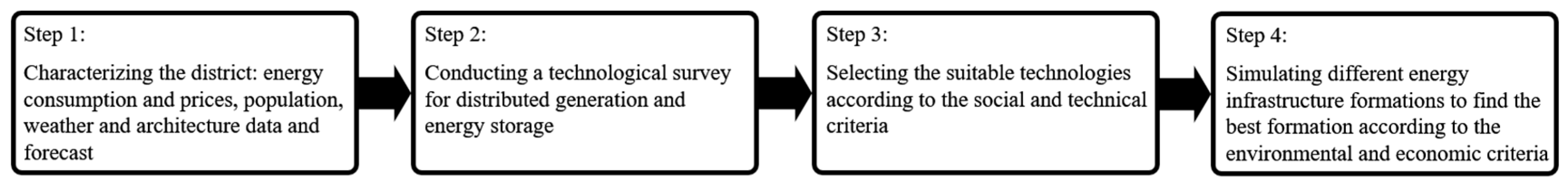
In order to achieve the research goal for building a comprehensive model for urban energy infrastructure design, a four-step methodology was suggested based on a similar concept suggested in [11]. However, in order to account for all four aspects of sustainability, the suggested model includes a combined qualitative and quantitative evaluation. The methodology is summarized in Figure 1. The first step of the methodology is characterization of the urban district. This includes gathering data regarding energy consumption history, population, architecture, energy policy, energy prices and weather history of the district and its area, and future energy consumption and weather estimations. The second step of the methodology is conducting a techno-logical survey on state-of-the-art commercial technologies for distributed generation (DG) and energy storage (ES). The third step is selecting technologies suitable for a given infrastructure according to social and technical criteria. Finally, the fourth step of the methodology involves selecting and using a design algorithm to simulate different energy infrastructure configurations and finding the best configuration according to the economic and environmental criteria. The simulations are based on the concept of microgrids which can switch between island mode, and connection to the national grid mode [11,14,16].

The first step of the methodology, as described above, requires cooperation with the district town planners in order to understand the available space inside the district for energy systems. For example, evaluating the available space for roof installed photovoltaic (PV) modules, should consider subtracting roof areas that are not exposed to direct solar irradiation due shading from taller nearby buildings or trees. Furthermore, the estimation of future energy consumption by the district and energy prices is based on regional trends, as suggested by [8,11] (i.e., gathering historical data in order to calculate the annual rate of change of energy consumption in the area of the district). The uncertainties associated with these estimated variables, including energy consumption by the district, energy prices, and weather data, are analyzed in a sensitivity analysis as presented by [9] and [17]. The sensitivity analysis is performed after the simulations in the fourth step of the methodology, and include investigation of the effect of changes in estimated variables on the economic and environmental outcome. In addition, the first step of the methodology includes gathering data regarding local energy policy. This includes laws preventing, promoting or requiring the use of certain technologies. Technologies that are forbidden according to the local policy are omitted from the following steps of the methodology.

In order to account for the four mentioned aspects of sustainability (technical, social, environmental, and economic), the model suggested in this project is based on two sets of criteria for design of urban energy infrastructure, which are being considered at different methodology steps. The first set includes social and technical criteria, which are prerequisites for the technological equipment. Thus, only technologies which satisfy the social and the technical criteria are considered in the fourth step of the methodology. This is carried out in order to include qualitative social and technical indicators, whereas the environmental and economic criteria include quantitative indicators only. The social and technical criteria are evaluated by using a simple multicriteria decision analysis, which includes giving weighted scores to the technological equipment reviewed in the second step of the methodology. This decision analysis was based on the site evaluation method presented in [8]. The weighted scores for the surveyed technologies are the sum of the multiplications of the grades that each technological equipment received for each indicator, and the weight of that indicator. The weights for the indicators are given subjectively by the decision makers, following their opinions regarding the level of importance of each indicator. The grades are given objectively based on the technological survey. The second set of criteria includes environmental and economic criteria, which are considered at the final step of the methodology. The presented model uses the CBA for evaluating infrastructure designs according to the economic criterion, and the LCA for evaluating designs according to the environmental criterion. The CBA is a commonly used tool for evaluating the benefits associated with certain costs. The presented model takes into account life-cycle costs and benefits, in order to evaluate all costs and benefits associated with the energy infrastructure [18]. The LCA is an evaluation of all GHG emissions associated with the energy infrastructure [7]. Moreover, the presented model evaluates designs according to each of the economic and environmental criteria separately, in order to allow decision makers to choose the most suitable design according to their subjective judging, while still being able to see the trade-off between the different criteria.

2.2. Design Criteria

2.2.1. Economic Criteria

As mentioned in the previous section, the economic aspect of the suggested model is based on the CBA for decision making, which takes under consideration the total costs and benefits associated with the energy infrastructure, over its life cycle. Since urban districts are basically energy consumers, the aim of the economic criterion in this model is to serve a tool for finding the infrastructure configuration with the lowest LCC (i.e., the highest cost savings). As such, three economic indicators which consider LCC are used: NPV, IRR, and LCOE. In order to evaluate savings, a basic infrastructure configuration is defined, where all of the needed electricity is purchased from the national grid.

NPV of an investment is the sum of total cash related to the investment discounted to the present value (i.e., the difference between the present value cash inflows and outflows over a period of time). Discounting enables to express future amounts of money in their present value. Generally, an investment is profitable if the NPV is positive, and the one having a bigger NPV is preferred [5]. NPV is calculated in terms of (all parameters are in USD) as [19]:

$$NPV={{\displaystyle \sum }}_{n=1}^{n=N}\frac{{\left(inflow\right)}_n-{\left(outflow\right)}_n}{{\left(1+r\right)}^n}-I_0,$$

(1)

where I₀ is the initial investment in year zero, (inflow)_n is the total cash inflow in year n, (outflow)_n is the total cash outflow in year n, r is the discount rate, and N is the life cycle duration. The cash inflow includes cost savings, defined as the difference between the total costs for electricity for the basic infrastructure configuration (purchasing all needed electricity from the national grid), and the total costs for electricity for the evaluated infrastructure configuration, in year n.

IRR is the discount rate which brings the NPV to zero (i.e., brings the cash inflows and outflows to break-even). As such, discount rates bigger than the IRR result in negative NPV which indicates that such investments are not profitable. Generally, a threshold discount rate is set for an investment, where IRR above it indicates its profitability. Hence, a higher IRR is more favorable. However, the IRR is generally not taken into account solely without considering the associated NPV, since the IRR signifies the level of confidence in the profitability of an investment, but the NPV signifies the actual level of the profits [20]. The IRR of the energy infrastructure is calculated by equating the NPV to zero [19]:

$$NPV=0={{\displaystyle \sum }}_{n=1}^{n=N}\frac{{\left(inflow\right)}_n-{\left(outflow\right)}_n}{{\left(1+IRR\right)}^n}-I_0,$$

(2)

where the cash inflow includes cost savings compared to using the basic infrastructure configuration as in Equation (1).

LCOE is the ratio between LCC and life cycle energy production in terms of unit money per unit energy produced (USD/kWh). LCOE is mostly used by power plants for calculation of the needed price of energy sold by the power plant in order to break-even the costs [21]. Nevertheless, LCOE in the suggested model was found to be a useful tool for comparing different energy infrastructure configurations to the basic one. In order to use LCOE for an urban district, it is described as the ratio between the NPV and the life cycle energy consumed. The numerator includes NPV regarding all energy sources and both purchased energy from the national grid and energy generated inside the district. This includes expenditures regarding electricity purchasing from the national grid, loan payments regarding purchased equipment, operational costs, and income from selling residual energy to the national grid. However, unlike the NPV calculation in Equation (1), the numerator does not include cost savings in order to enable the comparison of the actual energy cost between new configurations to the basic configuration. When comparing different energy infrastructure configurations, the calculated LCOE in terms of USD/kWh enables one to see the effects of different energy inputs on the cost of each unit energy consumed by the district. These effects on costs are included in the numerator, while the denominator remains the same for all infrastructure configurations. If the LCOE value is negative, it means that besides saving costs, the infrastructure was actually profitable. The LCOE was calculated as:

$$LCOE=\frac{I_0+{{\displaystyle \sum }}_{n=1}^{20}\left\{\left(P+O\&M_n+B_n-S_n\right)\left[\frac{1}{{\left(1+r\right)}^n}\right]\right\}}{{{\displaystyle \sum }}_{n=1}^{20}{E}_n},$$

(3)

where I₀ (USD) is the initial investment in year zero which include equity and installation costs, P (USD) is the yearly loan payment, O&M_n (USD) is the operation and maintenance costs in year n, B_n (USD) is the purchased electrical energy costs in year n from the national grid, S_n (USD) is the total income from selling residual energy to the national grid in year n, E_n (kWh) is the energy consumed in year n, and r is the discount rate.

The loan payment was assumed to be constant yearly and was calculated as the total loan multiplied by the capital recovery factor [16]:

$$P=L\cdot \left(\frac{i{\left(1+i\right)}^{RP}}{{\left(1+i\right)}^{RP}-1}\right),$$

(4)

where L (USD) is the total loan taken in year zero, i is the yearly interest rate, and RP is the number of years for repaying the loan.

2.2.2. Environmental Criteria

The connection between global warming and energy related GHG emissions [16,22], highlights the importance of minimizing the impact of energy infrastructure on the environment. Environmental impacts are classified into local and global ones. Local impacts are the effects that a certain facility has on the nearby area, such as air pollution and water and ground contamination. Global impacts are much larger in scale, affecting the climate. These impacts include GHG emissions which are related to global warming [23]. As presented in Section 1, environmental indicators used in previous urban energy projects included GHG emissions, land use, noise, pollutants emission, and water consumption. Since local impacts such as land use, noise, and pollutants emission have a direct effect on the well-being of the residents of the urban district, they are considered as part of the social criteria in the suggested model.

Accordingly, the suggested model uses GHG emissions for the environmental indicator. Furthermore, the evaluation of the environmental impact of energy infrastructure configurations is based on the LCA. The LCA considers entire life cycle GHG emissions, including the early stage of the manufacturing of the equipment used in the infrastructure. This prevents situations where an infrastructure configuration that has less operational GHG emissions than another but has more equipment manufacturing related GHG emissions, is considered to have lower environmental impact [7]. In order to evaluate the potential of environmental impact of different infrastructure configurations, the environmental indicator is presented in terms of GHG emission intensity per unit energy consumed by the district (i.e., the sum of total life cycle GHG emissions in terms of kgCO₂ equivalence, divided by the total life cycle consumed energy (kgCO₂/kWh)):

$$GHG=\frac{life cycle GHG emissions \left(kgC{O}_2\right)}{life cycle consumed energy \left(kWh\right)},$$

(5)

2.2.3. Social and Technical Criteria

Social criteria are inseparable from the infrastructure design for urban districts. The residents of the districts are the energy infrastructure end users, and it can have a significant impact on their well-being, which is their state of being happy and healthy. Well-being is divided into subjective and objective indicators. The objective well-being includes measures taken to maintain a reasonable quality of life, while the subjective one is individually determined and is related to how an individual feels about the objective well-being indicators, as presented in Section 1. The study of well-being is still ongoing, and indicators for the measurement of well-being are still being developed [12].

As mentioned in Section 2.1, the social criteria in the suggested model are defined as prerequisites for the technology used for electricity generation and ES inside the urban district. Following the technological survey in the second step of the methodology, the third step includes qualitative evaluation for the surveyed technologies according to the social indicators. The social indicators used in the suggested model include social acceptability, land use, noise levels, and air pollution. Although air pollution, excessive land use by the energy infrastructure and high noise levels from technological equipment were mostly considered as environmental criteria in previous projects, in the suggested model they are included in the social criteria due to their direct effect on the health and the general well-being of the residents [12,24].

Similarly to the social criteria, the third step includes qualitative evaluation of the technologies according to the technical indicators. Technical criteria provide tools for evaluation of energy infrastructure design from the prospective of the technical operation of the used equipment, as presented in Section 1. Surely, the main challenge for integrating renewable energy resources to the grid is their uncontrollable power generation which can lead to unsynchronized peaks of generation and consumption [14,16]. One method to avoid this mismatch is demand-side-management (DSM), which includes different methods for load shifting or load peak shaving on the energy consumption side [25,26]. Nevertheless, in this model the energy infrastructure is designed to meet the current energy needs of the urban district. In order to increase the acceptability of the model by the residents of the district, DSM was not considered in this model. As such, the technical criteria in this model included indicators regarding the workability of the DG and ES technologies. The technical indicators used in the suggested model include availability of resources, reliability, safety, efficiency and the level of commercial maturity. Among these indicators are the ones assumed to be the most crucial for disqualifying non-suitable technological equipment, such as the availability of resources and the level of commercial maturity.

2.3. Design Algorithm

The fourth step of the methodology in the suggested model includes simulating different energy infrastructure configurations to find the most suitable configurations according to the economic and environmental criteria, using a computer software. Various commercial software for simulating energy systems performance exist, among which the most common are the HOMER PRO by Homer Energy, the SYSTEM ADVISOR MODEL (SAM) by NREL, and the RETSCREEN by the Canadian Ministry of Natural Resources [8,11,27]. The simulations in SAM and HOMER PRO are based on hourly energy balance, making them more accurate than RETSCREEN which is based on annual average values. Nevertheless, HOMER PRO is more suitable for microgrids, as it can be used for grid connected and off-grid applications of hybrid distributed energy systems [17]. Alternatively, several previous projects have developed their own computer simulation tools instead of using commercial software [10,20,28]. HOMER PRO finds the best infrastructure configuration according to economic criteria only, and cannot be used to find the best configuration according to environmental evaluation. Furthermore, HOMER PRO does not consider GHG emissions associated with renewable energy systems in its calculations, which leads to incorrect environmental impact assessments. Moreover, HOMER PRO does not account for various factors which may have significant impact on the economic and environmental outcome, such as battery capacity fading due to aging, the need for a charge controller, battery self-discharging, etc. [29]. As such, in order to include comprehensive evaluations to find the best configurations economically and environmentally, a new algorithm was built using MATLAB software.

The algorithm used input data including hourly energy consumption of the district, local weather, prices, and technical specifications. Although energy consumption and production fluctuations may occur instantaneously, the simulations by the algorithm were based on hourly energy balance analysis due to the complexity of estimating energy consumption and production for short periods of time. As a result, time periods of one hour were assumed to be the shortest reliable time periods. Local weather data input includes hourly average solar irradiation, wind speed, ambient temperature and air density. Prices data input included electricity purchasing and selling prices in the region, equipment prices including initial investment, installation costs, and operation and maintenance costs, insurance costs, and financial data regarding loan interest rates, loan percentage of initial investment and discount rates. Technical data input included all necessary specifications for the used equipment, regarding its operation and associated GHG emissions.

There exists ongoing research of different methods of forecasting energy data, such as the hour-energy, one-step-ahead, one-hour-ahead, one-day-ahead forecasting, and newer methods which combine artificial intelligence [30,31,32,33]. Nevertheless, hour-energy balance based on trends from local historical data (i.e., energy consumption and weather data of the urban district and its area) can increase the acceptance of the infrastructure design by decision makers and residents of the district. That is due to its practicality, the simplicity of reading and understanding its output, and its connection to local historical trends [5,11]. As such, the simulations by the algorithm were based on hourly energy balance between consumption and supply. For every hour, the algorithm first used the energy generated inside the district in that period, to meet the demand in the same period. If the periodical demand is greater than the energy generated inside the district, the algorithm then used energy stored inside the district for back-up. However, if the stored energy was still insufficient to meet the demand, the algorithm uses energy purchased from the national grid. Accordingly, if periodical energy generation inside the district overcame the periodical demand, the excess energy was either stored inside the district, or sold to the national grid, depending on the infrastructure configuration. After, the algorithm calculates the environmental and the economic outputs. The environmental output was the ratio between total life cycle GHG emissions and the life cycle consumed energy, as depicted in Equation (5). Life cycle GHG emissions are the sum of the emissions associated with each of the used technologies according to their relative share in the energy mix of the current infrastructure configuration. The eco-nomic output included the LCOE, IRR and the NPV of the current infrastructure configuration, according to Section 2.2.1. The algorithm simulated different infrastructure configurations, based on a predefined range of usage levels of each energy generation or storage technology. The algorithm then found the configurations for which the GHG emissions and the LCOE were the minimal, and the configurations for which the IRR and NPV were maximal. This was carried out by MATLAB’s max/min functions. Lastly, the algorithm performed a sensitivity analysis in order to evaluate the effect of changes in several variables on the output. The algorithm was validated by comparing LCOE, NPV, IRR, and GHG emissions calculations by the algorithm and by using Excel software. The calculations compared were for ten different days throughout 20-year life cycle of a fictional district, while using different energy infrastructure configurations including national grid supply, PV generation, wind turbine generation, and lithium-ion battery storage. The algorithm scheme is presented in Figure 2.

3. Case Study

The model was implemented to design energy infrastructure for the Technion—IIT campus in Haifa, Israel, as a case study. This section presents the design following the four steps of the methodology in the suggested model.

3.1. First Step: Characterization of the Campus

The Technion campus is located in the city of Haifa, Israel, and situated on the north-eastern slopes of the Carmel Mountain. The campus functions as a multi-purpose urban district, as it consists of over 200 buildings, including dormitories, research facilities, sport facilities, commercial facilities and other office buildings, and its population reaches around 26,000 people daily. Moreover, the total roof area of the campus is 130,000 m² [34], and was all considered exposed to direct solar irradiation. Half hour electrical energy consumption data of the campus of one year from the 1 May 2018 to the 30 April 2019 was provided by courtesy of the campus electrical engineer, Itzik Romano. Yearly electrical energy consumption increase rate of 3% was considered for the campus throughout the life cycle of 20 years, based on the estimation made by the Technion [34] and the estimations for the entire country made by [35,36]. The uncertainty of the estimated rate has a direct effect on the economic and environmental output of the algorithm. Weather data were gathered from the Israeli Meteorological Service archive [37]. In order to fit the weather data to the corresponding energy consumption data, they were gathered for the same hours instead of considering typical meteorological year data. The weather data were considered as constant throughout the life cycle of 20 years. It is a source of severe uncertainty and has a direct effect on the economic and environmental output of the algorithm. Electricity purchasing rates for the campus vary according to the hour of the day, season of the year, and type of day (holiday, weekend, etc.). These electricity purchasing prices were updated for year 2020 and were considered as constant throughout the life cycle of 20 years. The uncertainties regarding the weather, electricity prices, and energy consumption data are discussed further in Section 3.5. Electricity selling prices to the national grid in Israel depend on the generation technology used and the size of the generation systems. As such, the prices were determined after selecting the used technology in the third step of the methodology, presented in Section 3.3.

3.2. Second Step: Technological Survey

Following the second step of the methodology, a technological survey for commercial DG and ES technologies was conducted. Important advantages and disadvantages for the surveyed DG and ES technologies are summarized in

Table 1. Advantages and disadvantages of distributed generation technologies.

Technology	Advantages	Disadvantages	Sources
Photovoltaic systems	‑ Use renewable resources ‑ Modular ‑ Easy to install and operate ‑ Low maintenance costs ‑ Can be installed on roofs ‑ Low purchasing costs ‑ Does not involve noises, air pollution or GHG emissions during operation	‑ Uncontrolled power generation ‑ Generation only during day-time ‑ Low efficiencies ‑ Unstable generation	[14,16,38,39,40,41]
Wind turbines	‑ Use renewable resources ‑ Modular ‑ Available in wide range of output ratings ‑ Can reach high efficiencies ‑ DO not require a lot of land and can be installed on roofs ‑ The operation involves no air pollution or GHG emissions ‑ Commercially mature	‑ High maintenance costs ‑ The operation involves loud noise ‑ The operation risks birds	[14,16,39,42]
Fuel cells	‑ High efficiencies ‑ The operation is silent ‑ The operation involves very little air pollution and no GHG emissions ‑ Can use renewable resources ‑ Available in wide range of output ratings	‑ High initial and operational costs ‑ Require high maintenance ‑ Commercially immature	[16,38,39]
Micro-turbines	‑ Dispatchable and the generation is controlled ‑ High energy density ‑ Reliable ‑ Can run on a wide variety of fuels ‑ Require less maintenance than other fossil fueled generation technologies	‑ Run on non-renewable fossil fuels ‑ The operation involves air pollution and GHG emissions ‑ The operation involves high noises	[38,39,43,44]
Reciprocating engine generators	‑ Can reach high efficiencies ‑ Available in wide range of output ratings ‑ Easy to install and operate ‑ Commercially mature ‑ Run on different common fuels ‑ Generation is controlled ‑ High energy density ‑ Can run on renewable resources	‑ Mostly run on non-renewable fossil fuels ‑ The operation involves air pollution and GHG emissions ‑ The operation involves high noises ‑ High maintenance costs	[38,39,44,45]
Biomass fueled generators	‑ Use renewable resources ‑ Can contribute to reduction of global GHG emissions and waste landfilling	‑ Involves air pollution and GHG emissions ‑ High initial and operational costs ‑ Can produce bad odors	[39,43,46,47,48]
Micro-hydroelectric plants	‑ Use renewable resources ‑ Generation is not hour-of-the-day dependent ‑ The operation does not involve air pollution and GHG emissions ‑ High efficiencies	‑ Require natural water bodies ‑ Require high maintenance ‑ Generation can be affected by seasonal weather	[38,39]

and

Table 2. Advantages and disadvantages of energy storage technologies.

Technology	Advantages	Disadvantages	Sources
Flywheels	‑ Can reach high efficiencies ‑ Long life cycles ‑ Fast charge and discharge ‑ The operation has low environmental impact ‑ Not affected by depth of discharge	‑ Low energy density ‑ High rates of self-discharge due to frictional losses ‑ Not very widespread ‑ The operation can involve loud noises	[49,50]
Pumped hydroelectric	‑ Can reach high efficiencies ‑ Long life cycles ‑ Commercially mature ‑ Fast discharge ‑ The operation involves no air pollution and no GHG emissions	‑ Requires suitable natural topography ‑ Can require changing the landscape ‑ The operation can involve loud noises	[49,51]
Compressed air	‑ Long life cycles ‑ Can reach high efficiencies ‑ Can reach high capacities	‑ Require natural caverns or building compressed air vessels ‑ The operation involves loud noise ‑ Not widespread	[49,51]
Supercapacitors	‑ High efficiencies ‑ Fast charge and discharge ‑ Long life cycles	‑ Low energy densities ‑ High self-discharge rates ‑ Not widespread	[49,50]
Lead acid batteries	‑ Can reach high efficiencies ‑ High energy density ‑ Commercially mature ‑ The operation involves no noise, air pollution or GHG emission	‑ Low energy density ‑ Highly affected by depth of discharge	[49,50,51,52]
Sodium-sulfur batteries	‑ Can reach high efficiencies ‑ High energy density ‑ Commercially mature ‑ The operation involves no noise	‑ The operation involves hazardous materials ‑ The operation requires high temperatures	[49,51,52]
Lithium-ion batteries	‑ Can reach high efficiencies ‑ Long cycle life ‑ High energy density ‑ Available in wide range of capacities ‑ Easy to install and operate ‑ Commercially mature ‑ The operation involves no noise, air pollution or GHG emission	‑ Highly affected by ambient temperature	[49,51,52,53,54]
Nickel cadmium batteries	‑ Commercially mature ‑ Fast charge and discharge ‑ The operation involves no noise ‑ Not affected by depth of discharge	‑ The operation involves hazardous materials ‑ Short cycle life	[49,52]
Vanadium reduction and oxidation flow batteries	‑ Fast response ‑ Long cycle life ‑ Can reach high efficiencies	‑ Low energy density ‑ Not widespread ‑ The operation requires using pumps	[49,51,52]
Hydrogen energy storage	‑ High energy densities ‑ Associated with low air pollution and ‑ GHG emissions	‑ Low round trip efficiencies ‑ Involves complicated processes ‑ Requires water supply	[49]
Superconducting magnetic energy storage	‑ Long cycle life ‑ High efficiencies ‑ Associated with low air pollution and GHG emissions ‑ Small self-discharge rates ‑ Fast charge and discharge	‑ Requires cryogenic cooling ‑ Not widespread	[49,50]
Thermal energy storage	‑ Associated with low air pollution and GHG emissions ‑ Commercially mature ‑ Can utilize waste heat from plants	‑ Low round trip efficiencies	[49,55]

, respectively.

3.3. Third Step: Selection of Suitable Technologies

The selection was based on the social and technical criteria which were prerequisites for the used technologies to be included in the simulations in the fourth step of the methodology. The following sections present the evaluation of the technologies reviewed in the technological survey. The evaluation was made in the form of a simple multicriteria decision analysis, where each technology was given grades for each of the weighted indicators that were presented in Section 2.2. The grades span between one and four according to the level of preference and were given objectively based on the technological survey. The weights were given subjectively, according to their importance in the opinion of the authors as part of the campus population. The total weighted score for each technology was calculated, and the technology that got the highest score was chosen for simulations. The evaluation results are presented in

Table 3. Social evaluation of distributed generation technologies (level of preference one to four).

DG Technology	Social Acceptability	Land Use	Noise Level	Air Pollution	Total Social Weighted Score
Photovoltaic systems	4	2	4	4	60
Wind turbines	3	4	3	4	60
Fuel cells	2	3	4	4	54
Micro-turbines	1	3	1	3	35
Reciprocating engine generators	1	3	2	2	33
Biomass fueled generators	1	3	2	2	33
Micro-hydroelectric plants	4	2	2	4	54
Weight	5	4	3	5

,

Table 4. Technical evaluation of distributed generation technologies (level of preference one to four).

DG Technology	Availability of Resources	Reliability	Safety	Efficiency	Level of Commercial Maturity	Total Technical Weighted Score
Photovoltaic systems	3	3	3	1	3	41
Wind turbines	1	2	3	1	3	27
Fuel cells	1	2	1	3	1	31
Micro-turbines	2	3	2	3	2	43
Reciprocating engine generators	3	3	2	3	3	48
Biomass fueled generators	3	2	1	2	1	36
Micro-hydroelectric plants	1	2	2	4	3	39
Weight	6	4	4	3	5

,

Table 5. Social evaluation of energy storage technologies (level of preference one to four).

Storage Technology	Social Acceptability	Land Use	Noise Level	Air Pollution	Total Social Weighted Score
Flywheels	3	2	2	4	49
Pumped hydroelectric	1	1	2	4	35
Compressed air	1	2	2	4	39
Supercapacitor	2	3	4	4	54
Lead acid batteries	3	2	4	4	55
Sodium sulfur batteries	3	3	4	4	59
Lithium-ion batteries	3	3	4	4	59
Nickel cadmium batteries	3	3	4	4	59
Vanadium redox batteries	3	2	3	4	52
Hydrogen storage	1	2	3	4	42
Superconducting magnetic storage	1	3	4	4	49
Thermal energy storage	2	2	3	4	47
Weight	5	4	3	5

,

Table 6. Technical evaluation of energy storage technologies (level of preference one to four).

DG Technology	Availability of Resources	Reliability	Safety	Efficiency	Level of Commercial Maturity	Total Technical Weighted Score
Flywheels	4	3	2	3	2	63
Pumped hydroelectric	1	2	2	3	3	46
Compressed air	4	2	2	2	2	56
Supercapacitor	4	2	3	3	1	58
Lead acid batteries	4	3	3	3	3	72
Sodium sulfur batteries	4	3	1	3	3	64
Lithium-ion batteries	4	3	3	3	3	72
Nickel cadmium batteries	4	3	1	3	3	64
Vanadium redox batteries	4	1	3	3	1	54
Hydrogen storage	1	2	2	1	3	40
Superconducting magnetic storage	4	2	2	3	1	54
Thermal energy storage	4	2	1	2	3	57
Weight	6	4	4	3	5

,

Table 7. Total scores for distributed generation technologies.

DG Technology	Total Weighted Score
Photovoltaic systems	101
Wind turbines	87
Fuel cells	85
Micro-turbines	78
Reciprocating engine generators	81
Biomass fueled generators	69
Micro-hydroelectric plants	93

and

Table 8. Total score for reviewed energy storage technologies.

DG Technology	Total Weighted Score
Flywheels	112
Pumped hydroelectric	81
Compressed air	95
Supercapacitor	112
Lead acid batteries	127
Sodium sulfur batteries	123
Lithium-ion batteries	131
Nickel cadmium batteries	123
Vanadium redox batteries	106
Hydrogen storage	82
Superconducting magnetic storage	103
Thermal energy storage	104

.

As seen from Table 7, PV systems received the highest score among the reviewed DG technologies. This outcome was expected, due to the high levels of solar irradiation in the area of the campus, the global trend toward increased installations of PV systems, and low air pollution and noise levels since it does not contain mechanical moving parts or use combustion. Furthermore, as seen from Table 8, the ES technologies which received the highest scores were batteries, excluding the vanadium redox flow batteries which suffer from low energy density which leads to high land use and low commercial maturity. The two highest scores were received by lead acid and lithium-ion batteries, mainly due to their high commercial maturity, low noise levels, and high social acceptability. Furthermore, lithium-ion batteries received a higher score than lead acid batteries due to their higher energy density. Sodium sulfur and Nickel cadmium batteries received lower scores due to hazard associated with toxic materials used by them.

3.4. Fourth Step: Simulation of Energy Infrastructure Configurations

The fourth step of the methodology included using an algorithm to simulate different configurations of energy infrastructure for the campus. As presented in the previous section, the DG and ES technologies selected were PV systems and lithium-ion batteries. In order to minimize land used by energy systems, the PV modules are installed on roofs. The algorithm simulated hourly energy balance for the life cycle of 20 years. The simulations were made for three different configurations for which different energy mixes were simulated, as presented in Figure 3. The first configuration was the basic configuration which included purchasing all needed electrical energy from the national grid. The second configuration included PV generation inside the campus with lithium-ion battery storage for excess generated energy and back up from the national grid. This configuration was simulated for different mixes which varied by the number of used batteries and the percentage of roof area covered by PV modules from the entire roof area of the campus. The number of batteries used spanned between 0 and 499, and the percentage of the roof area covered by PV modules was between 0 and 99. The third configuration included PV generation inside the campus while selling the excess energy to the national grid and purchasing back up from it. This configuration was simulated for different roof area coverage by PV modules as well, which also amounted up to 99%. PV generation and battery storage were simulated based on the formulae presented in Appendix B.

The equipment used in the simulations included several top products on the current energy systems market, as presented in Appendix A. Furthermore, input data for the simulations included energy consumption, weather, costs, technical data, and additional financial data. The last included national grid prices taken from [56], and equipment prices which are presented along with the equipment’s technical data in Appendix A. Electricity selling price to the national grid was based on the last tender made by the Israel Electricity Authority for roof installations of PV power plants, which determined the price of 0.066 USD/kWh [57] (Converted from NIS to USD based on exchange rate of 6 July 2020: 1 USD = 3.469 NIS). This price was considered constant throughout the lifecycle. Uncertainties regarding prices are discussed further in the sensitivity analysis in Section 3.5. The simulations included a loan with typical terms in the current Israeli energy market (i.e., a loan for 80% of the initial equipment costs, to be repaid in 10 years with constant yearly interest rate of 3.15%). Moreover, the economic calculations included in the simulations take into account a cautious yearly discount rate of 7%. GHG emissions from generation for the national grid were calculated according to the share of each fuel in the fuel mix. This was based on the fuel mix of 2018, and was assumed to be constant throughout the lifecycle. The mix included 66% natural gas, 30% coal (bituminous [58]), 1.1% diesel, and 2.9% renewables, mostly PV [59,60].

3.5. Simulation Results

Figure 4 shows hourly PV generation inside campus for three phenomena on three different days, and the matching hourly energy consumption by the campus. The values are taken from the first year of operation, with PV modules covering 99% of the campus roof area. The 6 June is an example of a clear sky sunny day, where the PV generation begins at sunrise around 5:00 a.m., peaks around noon, and ends at the sunset around 8:00 p.m. On 6 May, an interference by clouds blocking the sun from the PV modules is noticeable, where the PV generation increased before noon, then suddenly decreased around 11:00 a.m., and increased again after noon. The 6 December is an example for a cloudy day, where PV generation throughout the day was low. As can be seen from Figure 4, the energy consumption behavior of the campus fits that of an urban district where the majority of the population does not live in it, and rather populates the district during work hours. This makes peak consumption by the district almost synchronized with the peak PV generation.

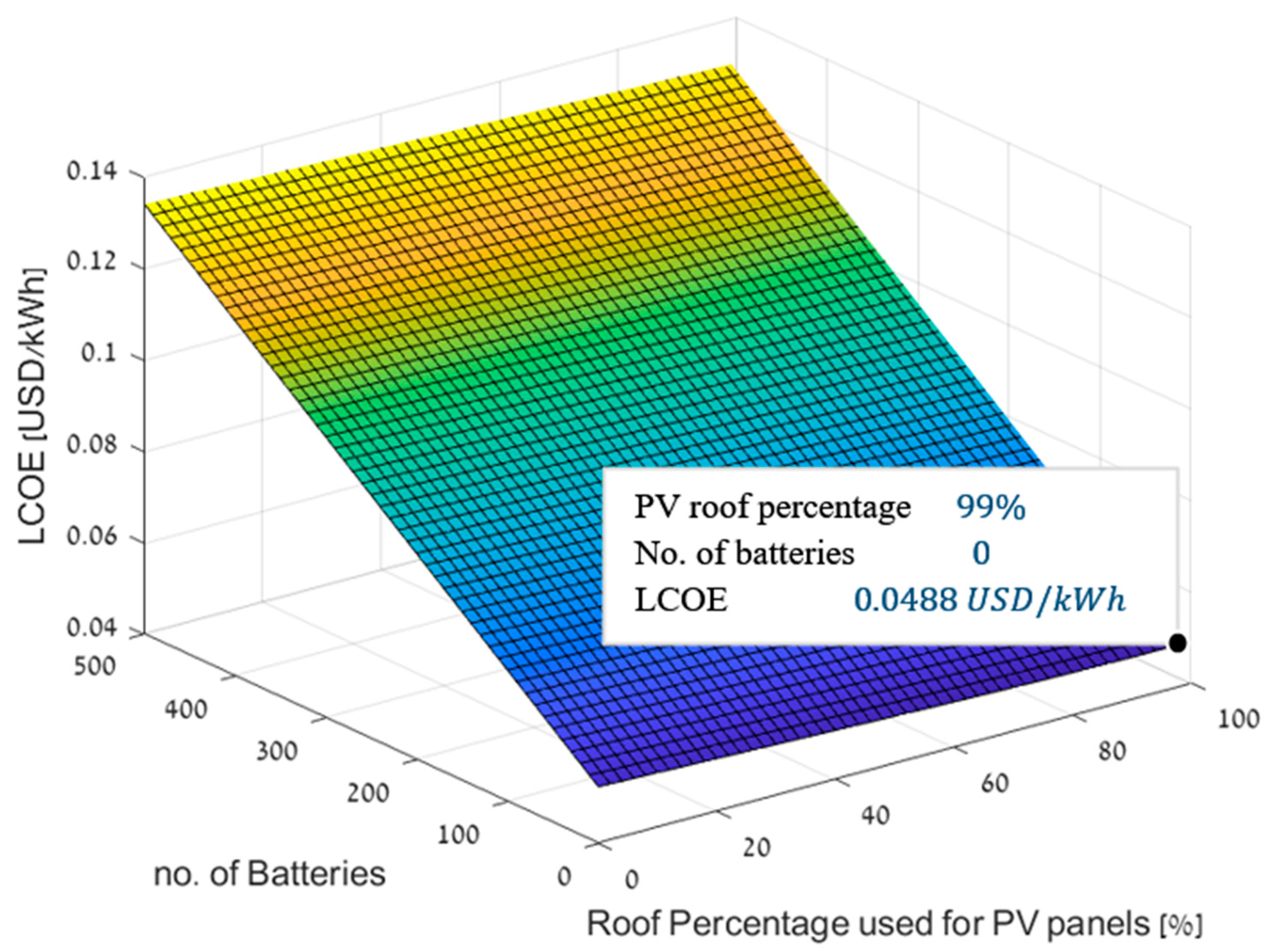
The LCOE for the basic configuration (configuration one) of buying all of the needed energy from the national grid, was 0.0521 USD/kWh. Furthermore, GHG emissions by configuration one were 0.2183 kgCO₂/kWh. LCOE results for configuration two, which included PV generation inside campus and residual ES in lithium-ion batteries are presented in Figure 5. This includes different usage levels of PV modules and batteries, as the percentage of the campus roof area covered with PV module ranges between 0 and 99%, and the number of batteries ranges between 0 and 499. As depicted in Figure 5, the lowest LCOE of 0.0488 USD/kWh was received for covering 99% of the campus roof area with PV modules while using no batteries. This is not equivalent to configuration three, since the residual energy is not sold. Furthermore, the LCOE increases as the number of used batteries increases. This is also presented in terms of the NPV for cost savings for configuration two shown in Figure 6, where the highest savings of about 7.812 million USD over the life cycle of 20 years were received for covering 99% of the campus roof area with PV modules while using no batteries. In addition, the NPV decreases as the number of used batteries increases, reaching negative values. Negative NPV means that for the used energy infrastructure configuration, the campus will pay more than it would if it were to use the basic infrastructure configuration (configuration one). As seen from Figure 5 and Figure 6, the economic worthwhileness of this configuration peaks when no batteries are used, and decreases with increasing the number of batteries used. This outcome results from the synchronization between the PV generation and the campus energy consumption. This synchronization is characterized by small amount of PV generation residuals for charging the batteries, as most of the PV generated energy is consumed by the campus immediately and not stored. This small amount of PV generation residuals is insufficient to justify the high prices of the batteries. Nevertheless, these figures show that this configuration becomes more worthwhile with increasing the number of PV modules used (i.e., the campus roof area covered with PV modules).

GHG emissions results for configuration two are presented in Figure 7. As can be seen in the figure, the lowest GHG emissions for configuration two were 0.1801 kgCOkgCO₂/kWh/kWh, and were received for using 12 batteries and covering 99% of the campus roof area with PV modules. Moreover, the GHG emissions increased with increasing the number of batteries used. This is mainly due to the high rates of GHG emissions involved in the manufacturing of the lithium-ion batteries along with the synchronization between the PV generation and the campus energy consumption mentioned above. Nevertheless, the GHG emissions decreased as the PV cell area used increased.

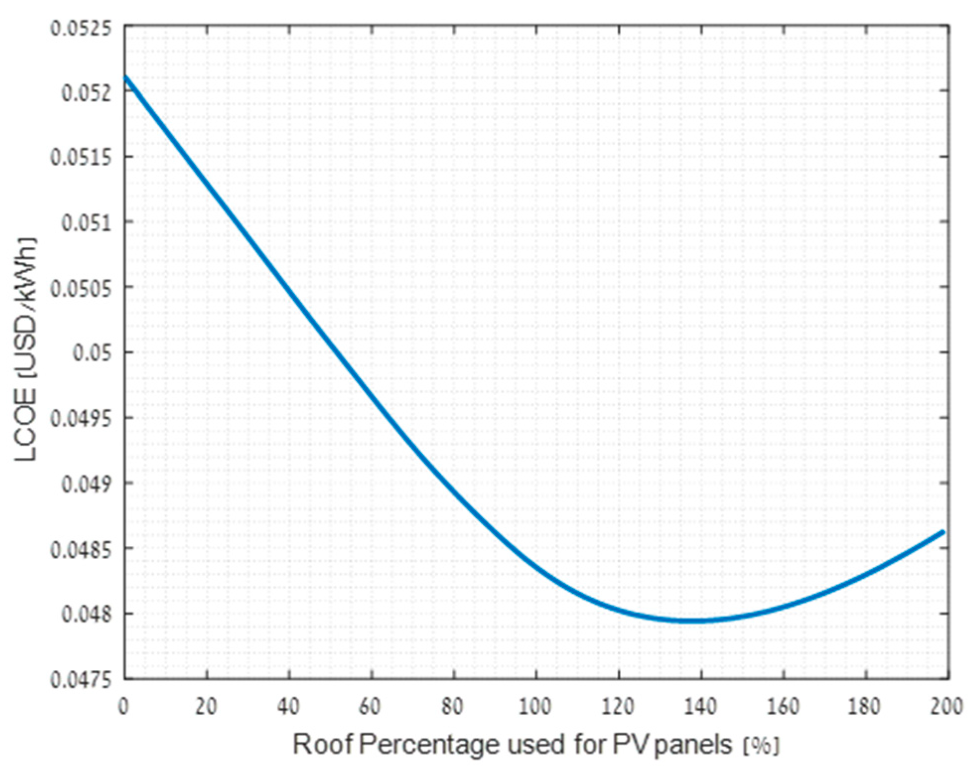
LCOE results for configuration three, which included PV generation inside campus and selling residual energy to the national grid are presented in Figure 8. The simulations included different usage levels of PV modules, expressed as the percentage of roof area of the campus, covered with PV modules. As presented from the figure, the LCOE decreased as the number of PV modules used increased. The lowest LCOE of 0.0483 USD/kWh was received for covering 99% of the roof area with PV modules. The same results can be seen in terms of the NPV for cost savings for configuration three presented in Figure 9, where the NPV increased as the number of PV modules used increased. The maximum NPV was 8.786 million USD and was received for covering 99% of the roof area with PV modules. Although Figure 8 shows that the LCOE for this configuration decreases monotonically with increasing percentage of roof covered with PV modules, this is not the case for PV cell area that exceeds the entire roof area of the campus. As seen from Figure 10, the LCOE for this configuration reaches a minimal value for using PV cell area that is equal to 138% of the campus roof area, and increases when increasing the PV cell area further. This outcome is important to prevent decision makers from having the notion that the more PV module used, the lower the costs. At 138% roof area covered with PV modules, all of the modules generate electricity that is consumed by the campus and meet the campus demand during generation hours. As such, in this point the PV generated electricity replaces entirely purchasing electricity from the national grid during high-rate hours, as presented in Appendix A. Beyond 138%, all electricity generated by additional PV modules is sold entirely to the national grid and is not consumed by the campus. Since the electricity selling price of 0.066 USD/kWh is much lower than electricity purchasing prices during high-rate hours which reach 0.257 USD/kWh, selling electricity is less economically worthwhile for the campus than consuming it. Hence, the LCOE increases for PV cell area exceeding 138% of the campus roof area, reducing costs savings for the campus. GHG emissions results for configurations three are presented in Figure 11, where the associated GHG emissions decreased as the number of PV modules used increased. This outcome is due to the relatively low emissions of PV modules manufacturing, compared to the emissions from fossil fuel generation as presented in Appendix A. In addition, residual PV generated electricity that is sold to the national grid replaces fossil fuel generated electricity supplied to it, contributing to GHG emissions reduction even further than the emissions associated with the energy consumed by the campus. The minimal GHG emissions were 0.1754 kgCO₂/kWh and were received for covering 99% of the campus roof area with PV modules.

In conclusion, configuration three with PV coverage of 99% of the campus roof area was found both the best economically and environmentally, receiving both the lowest LCOE and the lowest associated GHG emissions. The total energy consumed by the campus over the life cycle of 20 years was 2.35 TWh. This makes the difference of 0.0005 USD/kWh between the minimum LCOE values of configurations two and three result in a difference of over 1 million USD in total costs between the two configurations over the life cycle. The IRR for configuration three with PV coverage of 99% of the campus roof area, was 15.08%, according to Equation (2). This calculation signifies the worthwhileness of using this configuration and the confidence level of the economic simulations, as it is bigger than the discount rate of 7% considered in the simulations.

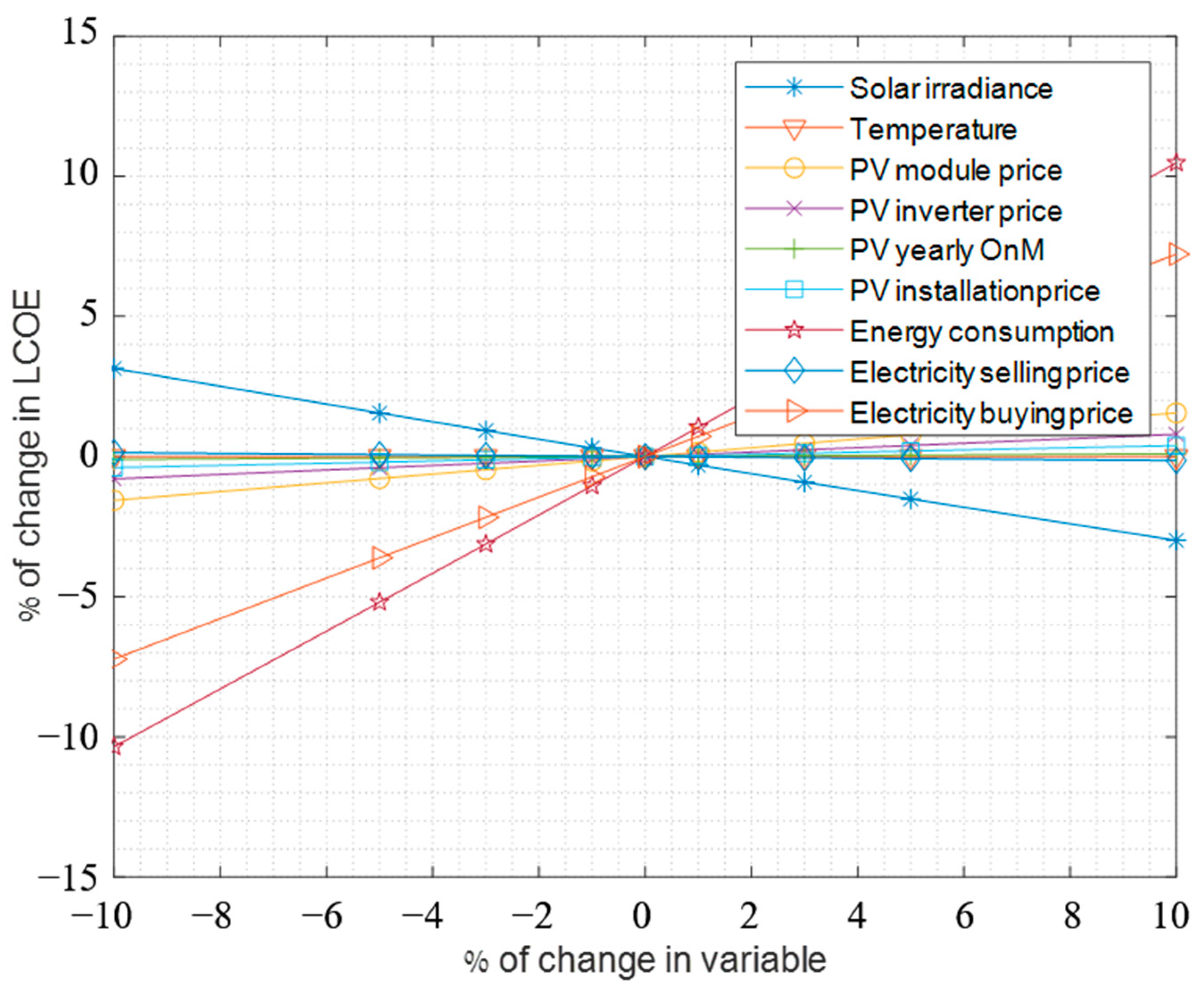
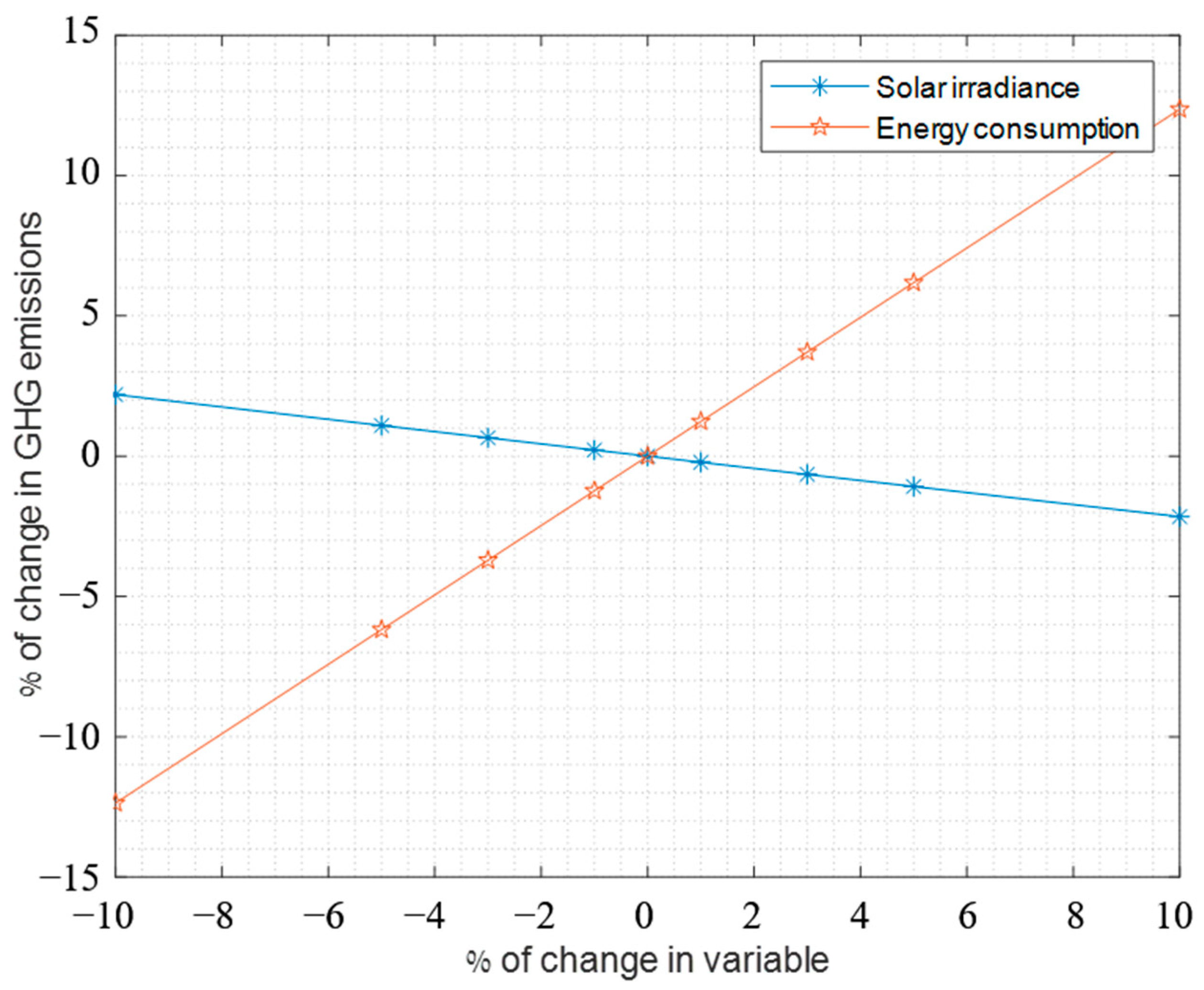
Lastly, a sensitivity analysis was performed in order to investigate the uncertainties concerning estimated variables in the simulations. The analysis was performed on configuration three with PV coverage of 99% of the campus roof area. Furthermore, the analysis included calculation of the effect of changes in estimated variables, on the LCOE and GHG emissions calculations. This was accomplished by performing the simulations several times, where each time one of the estimated values changed by a certain percentage. The results of the sensitivity analysis for the LCOE and GHG emissions are presented in Figure 12 and Figure 13, respectively. As presented in the sensitivity analysis, the estimation of energy consumption by the campus has the biggest effect on the LCOE. The second largest impact on the LCOE is from the estimation of electricity buying prices, and the third largest impact is from the estimation of solar irradiance. These effects on the LCOE are significant, since a change of 1% in the LCOE equals costs difference of about 1.1 million USD over the life cycle. The estimation of energy consumption by the campus had also had the biggest effect on the GHG emissions, as presented in Figure 13.

4. Discussion

The model presented in this research was built with an emphasis on accounting for the four aspects of sustainability discussed. In order to achieve that, the model includes a systematic approach, containing a four-step methodology. The first two steps of the methodology do not include sustainability evaluation measures. They rather include gathering data regarding the urban district for which the model is used to design an energy infrastructure, and data regarding commercial ES and DG technologies. Furthermore, the sustainability evaluation in the methodology is divided into two steps, where the social and technical evaluations are included in the third step, and the economic and environmental evaluations are included in the fourth step. This systematic approach can increase the sustainability of urban energy infrastructures as it allows designers to follow a certain “checklist” accounting for all necessary aspects.

The social and technical evaluations included in this model, are performed for the surveyed ES and DG technologies. As such, these evaluations act as prerequisites for the technologies used inside the district, hence, enabling meeting social and technical sustainability requirements prior to the design of the energy infrastructure. The social and technical evaluations are qualitative, based on a simple multicriteria decision analysis. As presented in Section 3.3, each technology received a weighted score, considering subjectively weighted criteria. Furthermore, each technology received an objective grade for each criterion, based on the technological survey. The use of subjective weights for the criteria enables these evaluations to be versatile according to the preference of decision makers. As such, it enables the evaluations to base the final weighted scores according to the level of importance of different social and technical criteria in the eyes of decision makers. This versatility is crucial for the model for the ability to be implemented in different locations, where decision makers have different priorities. Furthermore, the subjective evaluation can increase the acceptability of the infrastructure by the population as its end users, since their opinion can be taken into consideration regarding the used technologies [5]. However, the subjective weighting of the criteria can be exploited for promoting certain technologies. It gives decision makers the opportunity to give the weights in such manner that certain more favorable technologies receive the highest weighted scores. This gives an opening for corruption regarding the purchased equipment. In order to avoid that, it is important to have transparency in the weighting of the criteria, and to present any conflict of interest that decision makers may have regarding ES or DG technologies.

In the case of the Technion campus presented in this project, the weights for the criteria were given by the author as a member of the campus’ population. For the social criteria, social acceptability and air pollution received the highest weights due to the direct impact of air pollutants on the health of the local population [24], and the importance of reducing the potential for resistance from the residents towards the energy infrastructure [5]. As for the technical criteria, availability of resources received the highest weight of all of the social and technical criteria, since it was considered by the author as the most important criterion for using a certain technology in a certain location. Generally, scarcity of resources can make some technologies inoperable in desired locations, making all other technical advantages of the technologies less relevant. That is especially the case for renewable energy systems which rely on natural resources.

The environmental and economic evaluations in the model are performed using a computer algorithm to simulate different energy infrastructure configurations. In the case of the Technion campus, three different energy infrastructure configurations were simulated, each included different usage levels for DG and ES systems, as depicted in Figure 3. Although energy production from natural resources fluctuates much faster than hourly changes, the algorithm was based on hourly average calculations since most available weather data is measured in this manner. This can lead to instantaneous unpredicted gaps between the energy generation and demand, which can be overcome by purchasing backup from the national grid. As presented in Figure 4, the energy consumption behavior of the Technion campus matches that of a multipurpose urban district, where the majority of the population occupies it during work hours. As such, it is shown from this figure that the peak energy consumption of the campus is synchronized with the peak PV generation. It should be noted that this is not the case for every kind of urban districts. For example, peak energy consumption by districts where the majority of the population do live inside them, tends to be reached at later hours of the evening when residents get back home from work. Hence, peak PV generation in such districts mostly precedes the districts peak energy consumption by a few hours.

The economic evaluation was based on a CBA which included three indicators: the NPV, IRR, and LCOE, as described in Section 2.2.1. The benefits considered in the NPV and the IRR included cost savings compared to the basic configuration of buying all needed energy from the national grid. As such, the NPV provides a convenient tool for evaluating the economic worthwhileness of energy infrastructure configurations in terms of total cost savings over their life cycle, for which maximal values are desired. Furthermore, the LCOE provides a useful tool for comparison between the different infrastructure configurations, in terms of the levelized price of unit energy consumed by the district for which minimal values are desired. The IRR is used to assess the level of confidence in the economic calculations, providing the upper limit for the discount rate under which the NPV is positive. It should be noted that co-benefits from ancillary services that batteries are able to provide are not taken into account in this model. This is mainly due to their indirect impact on energy costs for the district, as their impact is mainly on the national grid. Moreover, this model does not take arbitrage profit of ES into account, since the concept of buying electricity from the national grid during low price hours and selling it back is restricted by law in Israel. The environmental evaluation in the model is based on calculating the amount of GHG emissions associated with unit energy consumed by the district. This accounts for both GHG emissions associated with fossil fuel generation for the national grid, and emissions associated with manufacturing of DG ES equipment. As such, the environmental evaluation is more comprehensive, considering all associated GHG emissions.

The sensitivity analysis presented in Figure 12 and Figure 13 emphasizes the large impact of energy consumption estimation on the LCOE and the associated GHG emissions. Other variables that were found to have a significant impact on the economic outcome include electricity buying prices, and solar irradiance. As such, decision makers need to note the large impacts that might be caused from unexpected changes in these estimated variables. For example, the COVID-19 pandemic in 2020 is expected to result with a significant decrease in the campus energy consumption compared to the estimated consumption, since the campus population during the pandemic outbreak decreases. As seen in the sensitivity analysis, such reduction in energy consumption results with lower LCOE and GHG emissions. The large impact of estimating electricity buying prices can be significant especially in countries where these prices are highly affected by global commodity price changes. For example, oil price changes can have a direct effect on electricity prices in countries where a large share of the electricity is generated using oil or oil products. However, electricity prices in other countries which rely mostly on local resources such as Israel relying on local natural gas as presented in Section 3.4, are expected to be less affected by global commodity price changes.

The developed model for the design of urban energy infrastructures proved to be a useful tool, enabling the design to account for the four aspects of sustainability. Dividing the national grid into smaller urban districts and implementing the model to design energy infrastructure for them, can increase the sustainability of the national grid substantially. That is since it enables the energy infrastructure design to be based on the needs of each specific district. Moreover, implementing the model for the national grid can lead to the integration of numerous DG systems. Such multiplicity of energy sources to the grid can increase the security of the energy supply compared to relying on only few central power plants of which operation stops can lead to large drops in energy supply to the grid [16]. Furthermore, energy supply security can be accounted for in the model directly by setting a guideline for usage levels of DG. This can be achieved by defining a minimal percentage of the district’s energy demand to be supplied from DG systems in the simulation algorithm. However, integrating renewable energy systems to the national grid can result with big ramp rates in energy demand from central fossil fueled power plants when the renewable generation stops. Moreover, it can lead to overflowing the grid when renewable generation overcomes energy demand. These phenomena are known as the “duck curve”, as was first described by the California Independent System Operator [61]. These phenomena can be overcome be using ES systems to store the excess renewable generated energy and use it whenever the renewable generation stops, in order to reduce the ramp rates in the demand from the central fossil fueled power plants [16]. Similar to energy security, dealing with the “duck curve” can be carried out directly in the model by setting a guideline for usage levels of ES systems. A comparison between state-of-the-art urban energy infrastructure design models and the model suggested in this study is presented in

Table 9. Urban energy infrastructure design models.

Authors	Presented Model	Sustainability Aspects Evaluated	Sustainability Evaluation Type	Judgment	Source
Pica et al. (2013)	A four-step methodology for planning distributed energy generation in urban districts	Economic and technical aspects	Quantitative	Objective	[11]
Ristimäki et al. (2013)	Evaluating the viability of sustainability of residential energy infrastructure	Economic and environmental aspects	Quantitative	Objective	[7]
Alkhalidi et al. (2018)	Designing energy and water infrastructure for a new sustainable city	Economic and environmental aspects	Quantitative	Objective	[8]
Becchio et al. (2018)	Designing a net-zero energy district	Fiscally quantifiable aspects of all four aspects of sustainability	Quantitative	Objective	[9]
Amado et al. (2017)	Designing net-zero cities	Technical aspects	Quantitative	Objective	[13]
This study	A four-step methodology for planning distributed energy generation in urban districts	All four aspects of sustainability	Combined quantitative and qualitative	Combined objective and subjective	-

.

It should be noted that some technical and social aspects, such as health issues resulting from local air pollution, may have an impact on the economic outcome. However, they were evaluated qualitatively in the second step of the methodology only. That is in order to focus on their technical and social implications, and to perform the economic evaluations for the urban district as an energy consumer with direct costs and benefits only. One uncertainty that this model does not consider and should be noted is unexpected policy changes regarding the energy sector. Governmental policy can change by making new laws that could affect the energy infrastructure directly. For example, the laws that prevent installations of certain technologies, or even require installations of some technologies [62]. Another point that needs to be noted is the model’s inability to simulate energy management for intervals shorter than one hour as is conducted by a smart grid control. Future work for elaborating the model may include an in district smart grid control. In addition, future work may include simulations of integrating different technologies in different steps during the life cycle of the infrastructure, which could allow the model to consider new developed technologies, or governmental policy changes. Furthermore, future elaboration of the model can include other indicators to the environmental evaluation, which include environmental impact in areas other than the district itself. This includes local pollution from equipment factories, and soil and water contamination from disposal of energy equipment. Further elaboration for the model can include energy mix for several DG methods in locations where resources are available. Moreover, future work may include the use of different time-series and artificial intelligence methods for forecasting and also for real time energy management. There exists ongoing research for integrating these methods for forecasting mainly energy consumption [30,31,32,33,63,64,65]. Such methods can be implemented in the suggested model and be used in the first step of the methodology for forecasting the urban district’s energy consumption and weather data, as well as in the fourth step for energy generation from DG equipment and real-time energy management. The use of such methods can increase the accuracy of forecasting and add the optimization of energy management inside the district.

5. Conclusions

The model developed in this research proved to be a comprehensive and versatile tool for designing urban energy infrastructure. The model accounts for the four aspects of sustainability: technical, social, economic, and environmental. This is carried out by following a four-step methodology, where the first step includes the characterization of the district and the second step included a conduction of a technological survey for commercial DG and ES technologies. The third step includes social and technical evaluations for the surveyed technologies, and the fourth step includes environmental and economic evaluations for different energy infrastructure configurations. The economic and environmental evaluations are performed by simulating hourly energy balance for the different infrastructure configurations for their life cycle. The importance of accounting for all four aspects of sustainability was emphasized, as it reduces the risk of far-reaching implications from omitted aspects which can risk the sustainability of the infrastructure. The main advantages of the proposed model are its versatility, systematic approach, comprehensive sustainability evaluation, and enabling public engagement. The main shortcomings of the proposed model include its inability to account for sudden governmental policy changes, and not considering environmental pollution in areas other than the district itself.

The model was implemented for the design of energy infrastructure for the Technion campus in Haifa as a case study. PV systems and Li-ion batteries were found to be the most suitable DG and ES technologies for the campus, according to the social and technical evaluations. Furthermore, three energy infrastructure configurations were simulated for the campus including different usage levels for the used equipment. The lowest LCOE for configuration two, which included PV generation inside the campus and Li-ion batteries for ES, was 0.0488 USD/kWh for covering 99% of the campus roof area with PV modules and using no batteries. The lowest GHG emissions for this configuration were 0.1801 kgCO₂/kWh for the same PV covering and using 12 batteries. The LCOE and GHG emissions for this configuration increased when increasing the number of batteries used, surpassing the values which were received for the basic configuration one which included buying all of the needed energy from the national grid (LCOE of 0.0521 USD/kWh and GHG emissions of 0.2183 kgCO₂/kWh). Nevertheless, the best infrastructure configuration both economically and environmentally was configuration three, which included covering 99% of the campus roof area with PV modules and selling the residual generated energy to the national grid. The LCOE for this configuration was 0.0483 USD/kWh and the GHG emissions were 0.1754 kgCO₂/kWh. In conclusion, using this configuration can save the campus over 8 million USD and reduce the campus’ contribution to GHG emissions by over 19% during the life cycle of 20 years compared to the basic configuration. The IRR for this configuration was 15.08% which signifies the economic worthwhileness of using this configuration and the high level of confidence in the outcome of the economic evaluations where a discount rate of 7% was assumed. The sensitivity analysis performed for estimated variables showed that energy consumption estimation has the biggest impact on both the environmental and economic outcomes and should be taken into account by decision makers.

References

- IEA—International Energy Agency. Energy Technology Perspectives 2016; IEA: Paris, France, 2016. [Google Scholar]
- United Nations, The Population Division of the Department of Economic and Social Affairs. World Urbanization Prospects: The 2018 Revision; United Nations: New York, NY, USA, 2019; ISBN 9789211483192. [Google Scholar]
- Becchio, C.; Bottero, M.; Corgnati, S.P.; Dell’Anna, F. A MCDA-Based Approach for Evaluating Alternative Requalification Strategies for a Net-Zero Energy District (NZED). In Multiple Criteria Decision Making: Applications in Management and Engineering; Zopounidis, C., Doumpos, M., Eds.; Springer International Publishing: Cham, Switzerland, 2017; pp. 189–211. ISBN 9783319392929. [Google Scholar]
- Sahely, H.R.; Kennedy, C.A.; Adams, B.J. Developing sustainability criteria for urban infrastructure systems. Can. J. Civ. Eng. 2005, 32, 72–85. [Google Scholar] [CrossRef] [Green Version]
- Wang, J.J.; Jing, Y.Y.; Zhang, C.F.; Zhao, J.H. Review on multi-criteria decision analysis aid in sustainable energy decision-making. Renew. Sustain. Energy Rev. 2009, 13, 2263–2278. [Google Scholar] [CrossRef]
- Strantzali, E.; Aravossis, K. Decision making in renewable energy investments: A review. Renew. Sustain. Energy Rev. 2016, 55, 885–898. [Google Scholar] [CrossRef]
- Ristimäki, M.; Säynäjoki, A.; Heinonen, J.; Junnila, S. Combining life cycle costing and life cycle assessment for an analysis of a new residential district energy system design. Energy 2013, 63, 168–179. [Google Scholar] [CrossRef]
- Alkhalidi, A.; Qoaider, L.; Khashman, A.; Al-Alami, A.R.; Jiryes, S. Energy and water as indicators for sustainable city site selection and design in Jordan using smart grid. Sustain. Cities Soc. 2018, 37, 125–132. [Google Scholar] [CrossRef]
- Becchio, C.; Bottero, M.C.; Corgnati, S.P.; Dell’Anna, F. Decision making for sustainable urban energy planning: An integrated evaluation framework of alternative solutions for a NZED (Net Zero-Energy District) in Turin. Land Use Policy 2018, 78, 803–817. [Google Scholar] [CrossRef]
- Sitorus, F.; Brito-Parada, P.R. A multiple criteria decision making method to weight the sustainability criteria of renewable energy technologies under uncertainty. Renew. Sustain. Energy Rev. 2020, 127, 109891. [Google Scholar] [CrossRef]
- Pica, C.; Leites, T.; Tumelero, F.; Trentin, R. Planning of Sustainable Urban Districts based on Smart Micro-Grids Concept: A Case Study in Brazil. In Proceedings of the ENERGY 2013: The Third International Conference on Smart Grids, Green Communications and IT Energy-Aware Technologies, Lisbon, Portugal, 24 March 2013; pp. 21–27. [Google Scholar]
- Hiscock, R.; Mudu, P.; Braubach, M.; Martuzzi, M.; Perez, L.; Sabel, C. Wellbeing impacts of city policies for reducing greenhouse gas emissions. Int. J. Environ. Res. Public Health 2014, 11, 12312–12345. [Google Scholar] [CrossRef]
- Amado, M.; Poggi, F.; Amado, A.R.; Breu, S. A cellular approach to Net-Zero energy cities. Energies 2017, 10, 1826. [Google Scholar] [CrossRef] [Green Version]
- Akinyele, D.; Belikov, J.; Levron, Y. Challenges of microgrids in remote communities: A STEEP model application. Energies 2018, 11, 432. [Google Scholar] [CrossRef] [Green Version]
- Tomc, E.; Vassallo, A.M. Community Renewable Energy Networks in urban contexts: The need for a holistic approach. Int. J. Sustain. Energy Plan. Manag. 2015, 8, 1–12. [Google Scholar] [CrossRef]
- Randolph, J.; Masters, G.M. Energy for Sustainability, 2nd ed.; Island Press: Washington, DC, USA, 2018. [Google Scholar]
- Kreith, F.; Goswami, D.Y. Energy Management and Conservation Handbook, 2nd ed.; CRC Press: Boca Raton, FL, USA, 2017. [Google Scholar]
- Allan, G.; Eromenko, I.; Gilmartin, M.; Kockar, I.; McGregor, P. The economics of distributed energy generation: A literature review. Renew. Sustain. Energy Rev. 2015, 42, 543–556. [Google Scholar] [CrossRef] [Green Version]
- Bhattacharyya, S.C. Energy Economics: Concepts, Issues, Markets and Governance, 2nd ed.; Springer: London, UK, 2019; ISBN 9781351626200. [Google Scholar]
- Yan, J.; Yang, Y.; Elia Campana, P.; He, J. City-level analysis of subsidy-free solar photovoltaic electricity price, profits and grid parity in China. Nat. Energy 2019, 4, 709–717. [Google Scholar] [CrossRef]
- Nuclear Energy Agency and International Energy Agency. Projected Costs of Generating Electricity; IEA: Paris, France, 2015. [Google Scholar]
- IPCC. Climate Change 2014: Synthesis Report. Contribution of Working Groups I, II and III to the Fifth Assessment Report of the Intergovernmental Panel on Climate Change; IPCC: Geneva, Switzerland, 2014.
- Bai, X. Integrating Global Environmental Concerns into Urban Management. J. Ind. Ecol. 2007, 11, 15–29. [Google Scholar] [CrossRef]
- World Health Organization. WHO Air Quality Guidelines for Particulate Matter, Ozone, Nitrogen Dioxide and Sulfur Dioxide: Global Update 2005; World Health Organization: Copenhagen, Denmark, 2005; ISBN 9289021926. [Google Scholar]
- Aghajani, G.R.; Shayanfar, H.A.; Shayeghi, H. Demand side management in a smart micro-grid in the presence of renewable generation and demand response. Energy 2017, 126, 622–637. [Google Scholar] [CrossRef]
- Palensky, P.; Dietrich, D. Demand side management: Demand response, intelligent energy systems, and smart loads. IEEE Trans. Ind. Inform. 2011, 7, 381–388. [Google Scholar] [CrossRef] [Green Version]
- Tomc, E.; Vassallo, A.M. The effect of individual and communal electricity generation, consumption and storage on urban Community Renewable Energy Networks (CREN): An Australian case study. Int. J. Sustain. Energy Plan. Manag. 2016, 11, 15–32. [Google Scholar] [CrossRef]
- Mehleri, E.D.; Sarimveis, H.; Markatos, N.C.; Papageorgiou, L.G. Optimal design and operation of distributed energy systems: Application to Greek residential sector. Renew. Energy 2013, 51, 331–342. [Google Scholar] [CrossRef]
- HOMER ENERGY HOMER PRO Documentation. Available online: https://www.homerenergy.com/products/pro/docs/3.9/solving_problems_with_homer.html (accessed on 20 July 2020).
- Raza, M.Q.; Khosravi, A. A review on artificial intelligence based load demand forecasting techniques for smart grid and buildings. Renew. Sustain. Energy Rev. 2015, 50, 1352–1372. [Google Scholar] [CrossRef]
- Bu, S.-J.; Cho, S.-B. Time Series Forecasting with Multi-Headed Attention-Based Deep Learning for Residential Energy Consumption. Energies 2020, 13, 4722. [Google Scholar] [CrossRef]
- Cheng, C.H.; Wei, L.Y. One step-ahead ANFIS time series model for forecasting electricity loads. Optim. Eng. 2010, 11, 303–317. [Google Scholar] [CrossRef]
- Khan, Z.A.; Khalid, A.; Javaid, N.; Haseeb, A.; Saba, T.; Shafiq, M. Exploiting Nature-Inspired-Based Artificial Intelligence Techniques for Coordinated Day-Ahead Scheduling to Efficiently Manage Energy in Smart Grid. IEEE Access 2019, 7, 140102–140125. [Google Scholar] [CrossRef]
- Technion. TechCity21—Strategic Master Plan for the Technion Campus until 2045; Technion: Haifa, Israel, 2017. [Google Scholar]
- Galo, L. A Long-Term Forecast of Electricity Demand in Israel; Research Department, Bank of Israel: Jerusalem, Israel, 2017. [Google Scholar]
- Herzog, C. Electricity Sector Forecast; BDO: Tel Aviv, Israel, 2017. [Google Scholar]
- Israel Meteorological Service IMS Data Archive. Available online: https://ims.data.gov.il/ims/1 (accessed on 29 May 2019).
- Willis, H.L.; Scott, W.G. Distributed Power Generation; Willis, H.L., Ed.; CRC Press: Boca Raton, FL, USA, 2000; ISBN 9780824703363. [Google Scholar]
- Bansal, R. Handbook of Distributed Generation: Electric Power Technologies, Economics and Environmental Impacts; Springer: Berlin/Heidelberg, Germany, 2017; ISBN 9783319513430. [Google Scholar]
- McEvoy, A.; Markvart, T.; Castaner, L. Practical Handbook of Photovoltaics: Fundamentals and Applications, 2nd ed.; Elsevier: Waltham, MA, USA, 2012. [Google Scholar]
- IEEE. IEEE Std 1562-2007: IEEE Guide for Array and Battery Sizing in Stand-Alone Photovoltaic (PV) Systems; IEEE: New York, NY, USA, 2008; ISBN 9780738153568. [Google Scholar]
- Hau, E. Wind Turbines, 3rd ed.; Springer: Berlin/Heidelberg, Germany, 2013; ISBN 0824715098. [Google Scholar]
- Akorede, M.F.; Hizam, H.; Pouresmaeil, E. Distributed energy resources and benefits to the environment. Renew. Sustain. Energy Rev. 2010, 14, 724–734. [Google Scholar] [CrossRef]
- Pepermans, G.; Driesen, J.; Haeseldonckx, D.; Belmans, R.; D’haeseleer, W. Distributed generation: Definition, benefits and issues. Energy Policy 2005, 33, 787–798. [Google Scholar] [CrossRef]
- Heywood, J.B. Internal Combustion Engine Fundamentals, 1st ed.; McGraw-Hill: New York, NY, USA, 1988; ISBN 9781260116106. [Google Scholar]
- Sanscartier, D.; Maclean, H.L.; Saville, B. Electricity Production from Anaerobic Digestion of Household Organic Waste in Ontario, Techno-Economic and GHG Emission Analyses. Environ. Sci. Technol. 2012, 46, 1233–1242. [Google Scholar] [CrossRef]
- Holm-Nielsen, J.B.; Al Seadi, T.; Oleskowicz-Popiel, P. The future of anaerobic digestion and biogas utilization. Bioresour. Technol. 2009, 100, 5478–5484. [Google Scholar] [CrossRef]
- Liu, Q.; Li, M.; Chen, R.; Li, Z.; Qian, G.; An, T.; Fu, J.; Sheng, G. Biofiltration treatment of odors from municipal solid waste treatment plants. Waste Manag. 2009, 29, 2051–2058. [Google Scholar] [CrossRef]
- Aneke, M.; Wang, M. Energy storage technologies and real life applications—A state of the art review. Appl. Energy 2016, 179, 350–377. [Google Scholar] [CrossRef] [Green Version]
- Tan, X.; Li, Q.; Wang, H. Advances and trends of energy storage technology in Microgrid. Int. J. Electr. Power Energy Syst. 2013, 44, 179–191. [Google Scholar] [CrossRef]
- Sandia National Laboratories. DOE/EPRI Electricity Storage Handbook; Sandia National Laboratories: Albuquerque, NM, USA, 2015. [Google Scholar]
- Akinyele, D.; Belikov, J.; Levron, Y. Battery storage technologies for electrical applications: Impact in stand-alone photovoltaic systems. Energies 2017, 10, 1760. [Google Scholar] [CrossRef] [Green Version]
- Larcher, D.; Tarascon, J.M. Towards greener and more sustainable batteries for electrical energy storage. Nat. Chem. 2015, 7, 19–29. [Google Scholar] [CrossRef] [PubMed]
- Dunn, B.; Kamath, H.; Tarascon, J.M. Electrical energy storage for the grid: A battery of choices. Science 2011, 334, 928–935. [Google Scholar] [CrossRef] [Green Version]
- Alva, G.; Lin, Y.; Fang, G. An overview of thermal energy storage systems. Energy 2018, 144, 341–378. [Google Scholar] [CrossRef]
- The Israel Electricity Authority Tariff Book. Available online: https://pua.gov.il/Rates/Pages/default.aspx (accessed on 2 June 2020).
- The Israel Electricity Authority Resolution No. 7 (56807)—Results of Procedure No. 2 for Determining a Tariff for Electricity Generation in Photovoltaic Technology in Roofing Facilities. Available online: https://www.gov.il/he/departments/policies/07568 (accessed on 2 August 2020).
- The National Coal Supply Corporation of Israel Coal—Basic Facts. Available online: https://ncsc.co.il/?content=פחם-עובדות-בסיסיות (accessed on 8 June 2020).
- The Israel Electricity Authority. Report on State of Electricity Sector 2018; The Israel Electricity Authority: Jerusalem, Israel, 2019.
- Israel Ministry of Energy. Israel Energy Sector Review 2018; Israel Ministry of Energy: Jerusalem, Israel, 2020.
- California Independent System Operator What the Duck Curve Tells Us about Managing a Green Grid. Available online: https://www.caiso.com/Documents/FlexibleResourcesHelpRenewables_FastFacts.pdf (accessed on 27 October 2020).
- Elshurafa, A.M.; Farag, H.M.; Hobbs, D.A. Blind spots in energy transition policy: Case studies from Germany and USA. Energy Rep. 2019, 5, 20–28. [Google Scholar] [CrossRef]
- Yu, L.; Qin, S.; Zhang, M.; Shen, C.; Jiang, T.; Guan, X. A Review of Deep Reinforcement Learning for Smart Building Energy Management. IEEE Internet Things J. 2021, 8, 12046–12063. [Google Scholar] [CrossRef]
- Zhou, S.; Hu, Z.; Gu, W.; Jiang, M.; Zhang, X.-P. Artificial intelligence based smart energy community management: A reinforcement learning approach. CSEE J. Power Energy Syst. 2019, 5, 1–10. [Google Scholar] [CrossRef]
- Wang, H.; Lei, Z.; Zhang, X.; Zhou, B.; Peng, J. A review of deep learning for renewable energy forecasting. Energy Convers. Manag. 2019, 198, 111799. [Google Scholar] [CrossRef]
- CanadianSolar CanadianSolar KuBlack CS3K-300/305/310/315MS. Available online: https://www.canadiansolar.com/downloads?downid=613 (accessed on 8 June 2020).
- Yue, D.; You, F.; Darling, S.B. Domestic and overseas manufacturing scenarios of silicon-based photovoltaics: Life cycle energy and environmental comparative analysis. Sol. Energy 2014, 105, 669–678. [Google Scholar] [CrossRef]
- Schneider Electric Conext MPPT 80 600 Solar PV Charge Controller. Available online: https://solar.schneider-electric.com/product/conext-mppt-80-600/ (accessed on 8 June 2020).
- SolarEdge Three Phase Inverters. Available online: https://www.solaredge.com/products/pv-inverter/three-phase#/ (accessed on 8 June 2020).
- Tesla Powerpack. Available online: https://www.tesla.com/powerpack (accessed on 8 June 2020).
- Romare, M.; Dahllöf, L. The Life Cycle Energy Consumption and Greenhouse Gas Emissions from Lithium-Ion Batteries; IVL Swedish Environmental Research Institute: Stockholm, Sweden, 2017; ISBN 9789188319609. [Google Scholar]
- EIA—US Energy Information Administration. How Much Carbon Dioxide Is Produced When Different Fuels Are Burned. Available online: https://www.eia.gov/tools/faqs/faq.php?id=73&t=11 (accessed on 29 November 2020).
Figure 1.
Design methodology scheme.
Figure 2.
Design algorithm flow chart.
Figure 3.
Simulated energy infrastructure configurations: (1) national grid supply only; (2) PV generation, battery storage and national grid back up; (3) PV generation with national grid back up and selling residual energy.
Figure 4.
Hourly PV generation simulations and hourly energy consumption for three different days: (a) sunny day, (b) some clouds interference, and (c) cloudy day.
Figure 5.
Levelized cost of energy for configuration two.
Figure 6.
Net present value for configuration two.
Figure 7.
Greenhouse gas emissions for configuration two.
Figure 8.
Levelized cost of energy for configuration three.
Figure 9.
Net present value for configuration three.
Figure 10.
Levelized cot of energy for configuration three for PV cell area exceeding the campus roof area.
Figure 11.
Greenhouse gas emissions for configuration three.
Figure 12.
Sensitivity analysis for the levelized cost of energy of configuration three with PV coverage of 99% of the campus roof area.
Figure 13.
Sensitivity analysis for the greenhouse gas emissions of configuration three with PV coverage of 99% of the campus roof area.