
Forecasting Amazon Rain-Forest Deforestation Using a Hybrid Machine Learning Model


1
Grupo de Neurocomputación Biólogica, Departamento de Ingeniería Informática, Escuela Politécnica Superior, Universidad Autónoma de Madrid, 28049 Madrid, Spain
2
Grupo de Investigación Multidisciplinar en Sistemas de Información, Gestión de la Tecnonlogía e Innovación, Escuela Politécnica Nacional, Quito 170525, Ecuador
3
SI2Lab, Facultad de Ingeniería y Ciencias Aplicadas, Universidad de las Américas, Quito 170124, Ecuador
*
Author to whom correspondence should be addressed.
Sustainability 2022, 14(2), 691; https://0-doi-org.brum.beds.ac.uk/10.3390/su14020691
Submission received: 20 December 2021
/
Revised: 3 January 2022
/
Accepted: 7 January 2022
/
Published: 9 January 2022
(This article belongs to the Special Issue Neural Networks and Data Analytics for Sustainable Development)
Abstract
:The present work aims to carry out an analysis of the Amazon rain-forest deforestation, which can be analyzed from actual data and predicted by means of artificial intelligence algorithms. A hybrid machine learning model was implemented, using a dataset consisting of 760 Brazilian Amazon municipalities, with static data, namely geographical, forest, and watershed, among others, together with a time series data of annual deforestation area for the last 20 years (1999–2019). The designed learning model combines dense neural networks for the static variables and a recurrent Long Short Term Memory neural network for the temporal data. Many iterations were performed on augmented data, testing different configurations of the regression model, for adjusting the model hyper-parameters, and generating a battery of tests to obtain the optimal model, achieving a R-squared score of 87.82%. The final regression model predicts the increase in annual deforestation area (square kilometers), for a decade, from 2020 to 2030, predicting that deforestation will reach 1 million square kilometers by 2030, accounting for around 15% compared with the present 1%, of the between 5.5 and 6.7 millions of square kilometers of the rain-forest. The obtained results will help to understand the impact of man’s footprint on the Amazon rain-forest.
1. Introduction
In the last 20 years, the world has seen significant economic and productivity growth, but they have come at a great cost in terms of equity and sustainability, where sustainability is realized as our ability to pass on the assets necessary for future generations’ well-being [1,2]. With rising population and per capita consumption, one of the major concerns of our time is ensuring long-term sustainability. This is reflected in Rio + 20’s post-2015 development agenda, where the Sustainable Development Goals (SDGs) replaced the Millennium Development Goals [1]. Under this agenda, efforts to limit deforestation are rising worldwide as a result of climate change mitigation strategies, and have been promoted as one of the United Nations’ SDGs for the period 2015–2030 [3]. Target 15.2 (under Goal 15) was added to the SDGs to promote efforts to stop deforestation and promotes “the implementation of sustainable management of all types of forests, halt deforestation, restore degraded forests and substantially increase afforestation and reforestation globally” [4].
In recent years, debates have risen on the difficulties and potentials for sustainable agriculture and natural resource management, particularly of land, water, and forests. This is attributable, not only to a more prominent climate change agenda, which aims to reduce greenhouse gas emissions in order to keep global warming below 1.5 degrees Celsius, but also to the current SDGs agenda. Soil erosion, reduced water quality and supply, biodiversity loss, and increased carbon emissions are all consequences of forest conversion, i.e., the clearing of natural forests (deforestation) to use the land for another purpose [5]. In the face of these threatening scenarios, efforts to reduce deforestation are increasing globally as a result of climate change mitigation schemes, and it has recently been promoted as one of the United Nations’ 2015–2030 SDGs [3]. Deforestation in the Amazon is wreaking havoc on global climate, biodiversity, human health, and local and regional economies. In order to achieve Good Environmental Status and alleviate poverty, this difficult scenario needs to tackle a long-term sustainable use of the region’s resources in accordance with SDGs. Forest sustainability is addressed by at least eight of the 17 UN Sustainable Development Goals, with the primary goals being fighting desertification, halting biodiversity loss, and reversing land degradation [6].
The Amazon is recognized as the largest tropical rain forest in the earth, hosting 25% of the planet’s biodiversity [7]. It is one of the major responsibilities of climate regulation at a global level, as well an important source of tropospheric heat for general atmospheric circulation [7,8]. Due to the sustained deforestation in the last decades in the Amazon region, and considering the importance of Amazon vegetation and its impact on the global climate and weather, the deforestation is recognized as an issue to be solved in order to reduce their negative effects in this ecosystem and for sustainable development [9]. Since 2012 there has been an increase in deforestation rates in the Brazilian Amazon, regardless of the attempts to mitigate it. One of the principal reasons is the deficiency in deforestation control [10]. In 2015–2016 a high increment, about 29%, in the annual clearing rate of Brazil’s Amazon forest [10]. Despite all the efforts implemented by Brazil, which is an example for its policies in order to minimize CO emission, the deforestation and the elimination of autochthon vegetation is on the rise. Deforestation of the Brazilian Amazon is partly increased due to the lack of environmental policies to control practices related to illegal logging, farming, and mining. Infrastructure, commerce, debt, human capital investment, and resource-based economic expansion all exacerbate deforestation. Absolute and relative scarcities, as manifested by rising population pressures, food and land scarcities, fuel-wood dependency, and inequities in land access, are also important contributors in forest decline [11]. Major reforms in land-policy use are required, securing the foundations for the forest base’s long-term viability will require a two-pronged approach by development planners and policymakers, one that addresses not only the land-use practices that lead to the loss of tropical forests, but also the underlying social processes that cause this destruction [12,13].
Considering the relevance of deforestation in Amazon region and the necessity to research their rates and trends, the present work aims to make use of machine learning algorithms and data analytics techniques [14,15,16,17,18,19] to carry out an analysis of the human impact on Amazonian region [20,21]. Considering the Amazon importance on the planet and the excessive rain-forest lost, it is valid to analyzed the deforestation levels from historical data and predict it for the next years. Most works have focused in detecting deforestation impacts [22,23] and its triggers, as well as automating the task of detecting and mapping deforestation in the Amazon from satellite images [24], using mainly deep convolutional neural networks [25,26]. The present work focuses on forecasting deforestation, which is why the present research intends to predict its future behavior in order to serve as the basis for prospective studies. Forecasting a continuous value is an involved task. First, it is a regression problem, which is more complex to model than a classification one. Second, it is not possible to assume independence among observations, since there is a temporal dependence in the observed data. Third, there is not always the right amount of data available to build the model, thus forecasting the present and the future on past data that could be sparse is also an issue. All this makes time series forecasting a complex task to achieve. Recent works show that deep learning techniques for time series have proved to outperform traditional time series analysis methods. They have proved to be an effective solution to the aforementioned difficulties, given their capacity to automatically learn the temporal dependencies present in time series [27]. Thus, the main hypothesis of this work is that the Brazilian Amazon deforestation increase, can be modeled using a deep learning recurrent network model for the temporal data, together with a dense network for the static data. Together with the proper optimization of the model and data augmentation, the aforementioned difficulties can be addressed.
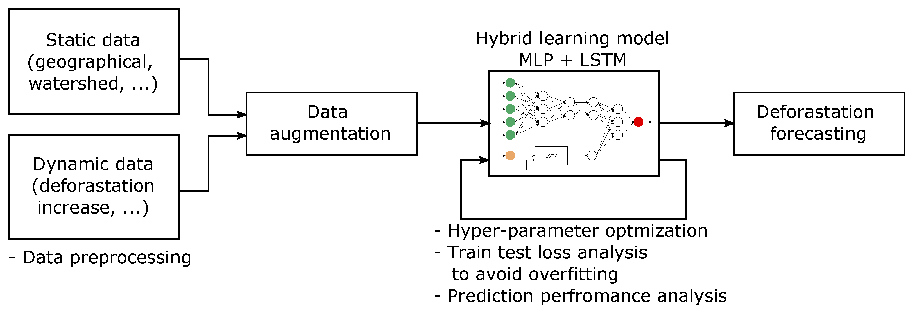
A hybrid learning method is proposed to predict deforestation rate in the Amazon rain-forest in the future decade. The workflow of the present research is depicted schematically in Figure 1. This study used a dense neural network, namely a multi-layer perceptron (MLP), the deforestation to model the static data and a long-short term memory (LSTM) network to model the temporal data. The research is based in a dataset which included information on about 760 municipalities, and their latitude, longitude, area, hydrography, non-forest area, and also included annual deforestation data for the last 20 years. Considering the variables typology, the designed model combines the MLP for fixed variables and recurrent LSTM neural networks for temporal variables. A data augmentation process has been carried out to generate synthetic data to train the model, which produced better results, as demonstrated by the hyper-parameter optimization process, where the amount of generated data was included. Once the best hyper-parameter optimization was found, the resulting model was used to model the deforestation increment from the observed data. A model loss analysis confirmed the appropriateness of the presented model to avoid over-fitting. A residual or error analysis is carried out to measure the performance of the model to evaluate the regression model.
The next sections are structured as follow. Section 2: Material and methods, describes the data and details the proposed machine learning model used in this work to predict the increment in deforestation of the Amazon rain forest. Section 3: Results, presents the data pre-processing methods and data augmentation carried out and present the experimental results, obtained for the model and the deforestation forecasting. Finally, in Section 4 Discussion and conclusions, as well as future works are exposed.
2. Materials and Method
2.1. Data Description
The data is composed of static variables with geographical and administrative information from 760 municipalities from Brazilian Amazon, and temporal data of yearly deforestation for each municipality. The collected data comprised the years between 2000 and 2020. Table 1 depicts the dataset variables, with the corresponding data types (measurement scale) and a description of each variable. The data comes from the TerraBrasilis [28] platform for the organization, access and use of geographic data for environmental monitoring. TerraBasilis was developed by The National Institute for Space Research (INPE) which is a research unit of the Brazilian Ministry of Science and Technology.
Figure 2 depicts the deforestation up to 2020 in yellow, and in orange the Brazilian Amazon biomass limits. The map, like the data, has been taken from TerraBrasilis [28]. It can be observed that in the south and east of the Amazon rainforest there is a higher degree of deforestation; this is in accordance with the number of municipalities in the region. Thus, it can be concluded that, whence more municipalities are, i.e., the more the human presence, greater is the deforestation.
The total deforestation in the last 20 years is depicted in Figure 3 for the Amazon states of Brazil. In the Figure 3a the Forest area of 2020 is compared to the Forest area that existed in 2000, and expressed as rate between 2020 and 2000. This rate, i.e., deforestation, can be expressed as the percentage of Forest lost, that occurred in the last 20 years for each state, and is presented in Figure 3b. The state with higher deforestation levels is Maranhão (MA) which lost around 56% its Forest area, from 68,806.3 km to 30,346.3 km for an area of 38,460 km of forest lost. Roraima (RR) is the next state that lost the most Forest in the period with 43% decrease, from 156,588.4 km to 88,778.64 km, for an area of 67,809.76 km of forest lost. However, the Forest area of the aforementioned state is smaller than states such as Pará (PA) and Amazon (AM), that lost 21% and 19%, respectively, but in absolute values represent a forest lost of (944,248.1–761,848.27) 182,399.83 km, and (1,462,388.9–1,343,017.65) 119,371.25 km, respectively. This latter values are substantially a larger forest lost for these states. A summary of the plots is presented in Table 2.
The annual increment in deforestation is shown in Figure 4a depicts the deforestation increment for each year from 2001 to 2020. Note that the reference year 2000 is not present, since this graph shows an increment, that is a difference between the actual and past year. A downward trend can be observed from 2000 to 2012, but from this minimum, an upward trend has been produced in the deforestation increment. Figure 4b depicts the cumulative deforestation from 2000 to 2020. The annual increment in deforestation will be predicted by the hybrid learning model, using both, the static and temporal data described in Table 1. If the deforestation increment is known, so is the cumulative deforestation by year, that will also be analyzed.
2.2. Hybrid Learning Model
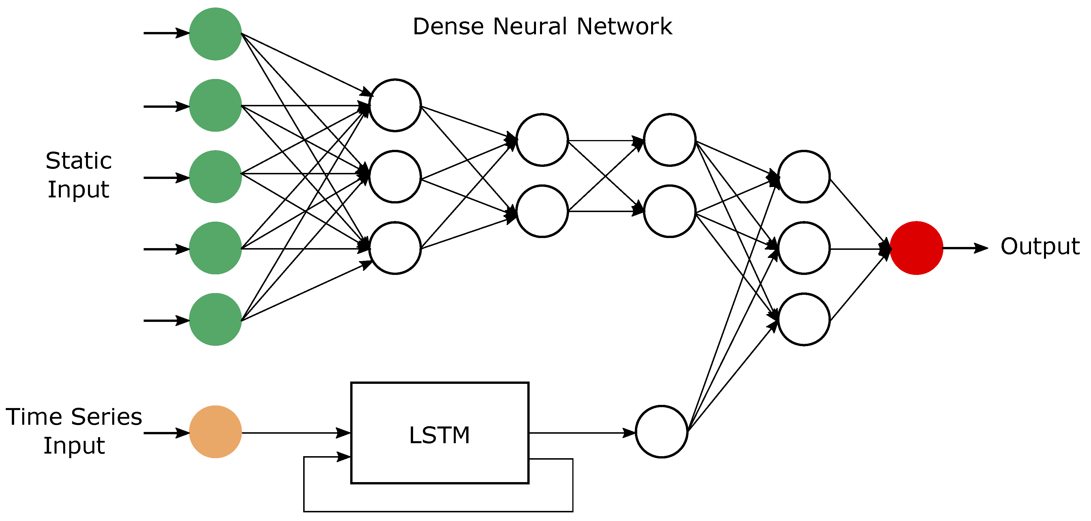
Figure 5 depicts a schematic representation of the hybrid learning model used to predict the increment in deforestation of the Amazon rain forest. A dense neural network, i.e., a Multi-layer perceptron (MLP), is used to process the neural static input variables described in Table 1. The dense network to model the static data can be expressed as follows:
where represents the static input and the dense network output.
The Long-short term memory (LSTM) model for the dynamic data (in Table 1) can be represented as
where represents the temporal input and the LSTM output. Note that the temporal model is multivariate, that is the deforestation increase will be forecasted on more than one time-dependent variable. Each variable depends not only on its past values but also has a dependency on other variables. This dependency is used for forecasting future values of deforestation. This is expressed in Equations (3) and (4) as matrices indicating the multidimensional nature of the temporal input, where . Given the temporal nature of the data used in the LSTM, Equation (2), can be expressed as follows:
where are the actual and past values of the time series, is the forecasted value, f represents the LSTM model, k is the window size used to perform the forecasting, and N is the number of observations (years) in the database. In the LSTM model k is an hyper-parameter to be optimized. As an example, Equation (3) for a windows size , can be written as:
Note that the indexation here, corresponds to a temporal index t.
Finally, an additional dense layer is added to the neural network to merge static and dynamic outputs for the deforestation prediction ,
The concatenation of the two models is schematically represented in Figure 5.
2.2.1. Dense Network: Multi-Layer Perceptron for Static Data
Figure 6 represents the basic computation unit of the Multi-layer perceptron (MLP), which will be used to model the static data. Each neuron computes the weighted sum of its input, the output of the node is obtained from a so called, activation function. This can be expressed in a matrix form, for the whole dense network in Figure 5, as follows:
represents the input matrix, where rows are the observed instances, and the columns the features in the data. is the weight matrix, is the weight vector for each node bias. is the activation function. The weights are calculated iteratively by the backpropagation algorithm [29,30] with the aim of reducing the error between an observed output y and the output of the network .
The backpropagation algorithm, can be summarized as follows. First, the input is feed-forwarded through the network, i.e., is calculated. Second, The error of the network is calculated, . The error is backpropagated through the network, and the responsibility in the error of each neuron in each layer is calculated. Third, the network weights are updated accordingly the neurons responsibility in the error. The backpropagation algorithm minimizes the error function using an optimization technique known as gradient descent. In the process the chain rule is applied to calculate partial derivatives, thus the activation function should be derivable.
Usual activation functions are relu, sigmoidal, soft-max, among others [31]. From a implementation perspective, a relu function is usually employed, given its lower computational cost. Also, the network is not fed with all the instances available. The neural network is required to learn from the entire training set, but, for computational reasons, generally the weights are not updated after evaluating all the instances. On the other hand, the entire training set is reordered randomly and divided into batches of a given size. The updating of weights is produced by applying the gradient descent using the elements of the batch.
2.2.2. Long-Short Term Memory for Temporal Data
The model in Figure 5 is comprised of two parts, the dense network (MLP) to model the static input to the static output , described above, and the LSTM network to model the temporal input to the temporal output , which is described as follows. Traditional Artificial Neural Networks (ANN), such as the MLP, build a direct mapping between the input and output data for the forecasting approach. The MLP does not consider the time correlation in a data sequence, so the ANN model is unable to capture the relationship between data and time. This restricts the application of the MLP in time series forecasting approaches. The use of the MLP for the static data, together with a Recurrent Neural Network (RNN), is proposed to overcome this disadvantage.
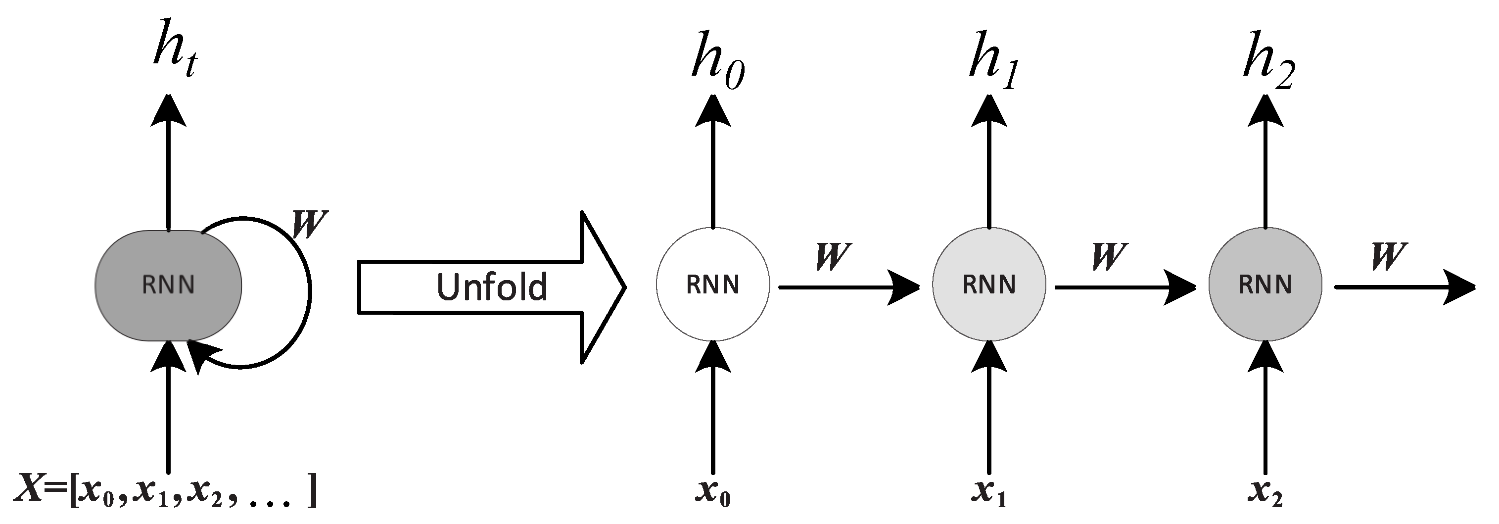
An RNN can be considered as multiple copies of the same network, each one of which transmits information to its successor in a loop, allowing the information to persist [32]. The RNN is represented schematically in Figure 7. The RNN receives a sequence of temporal inputs , , where k is the window size to perform the predicted forecast. First it receives the input and generates the output . In the next step, the inputs are and and the output is generated, which again serves as an input in the next step together with . This process is repeated successively until the last step, which receives the input and the output of the previous step to predict , which is the output of the model. Finally, a recurrent red evaluates each input and output of the previous step to generate the output hi and transmit it to the next step. All of the recurrent neuronal networks form a chain of repetitive modules of the neuronal network.
Then the training process of a RNN consists a forward pass and a backward pass. The forward pass of a RNN is the same as that of a MLP with a single hidden layer, except that activations arrive at the hidden layer from both the current external input and the hidden layer activations from the previous time steps. The backward pass to calculate weight derivatives for RNN is called back propagation through time (BPTT). Like standard backpropagation, BPTT consists of a repeated application of the chain rule. For a RNN, the loss function depends on the activation of the hidden layer not only through its influence on the output layer but, as aforementioned, through its influence on the hidden layer at the next time step.
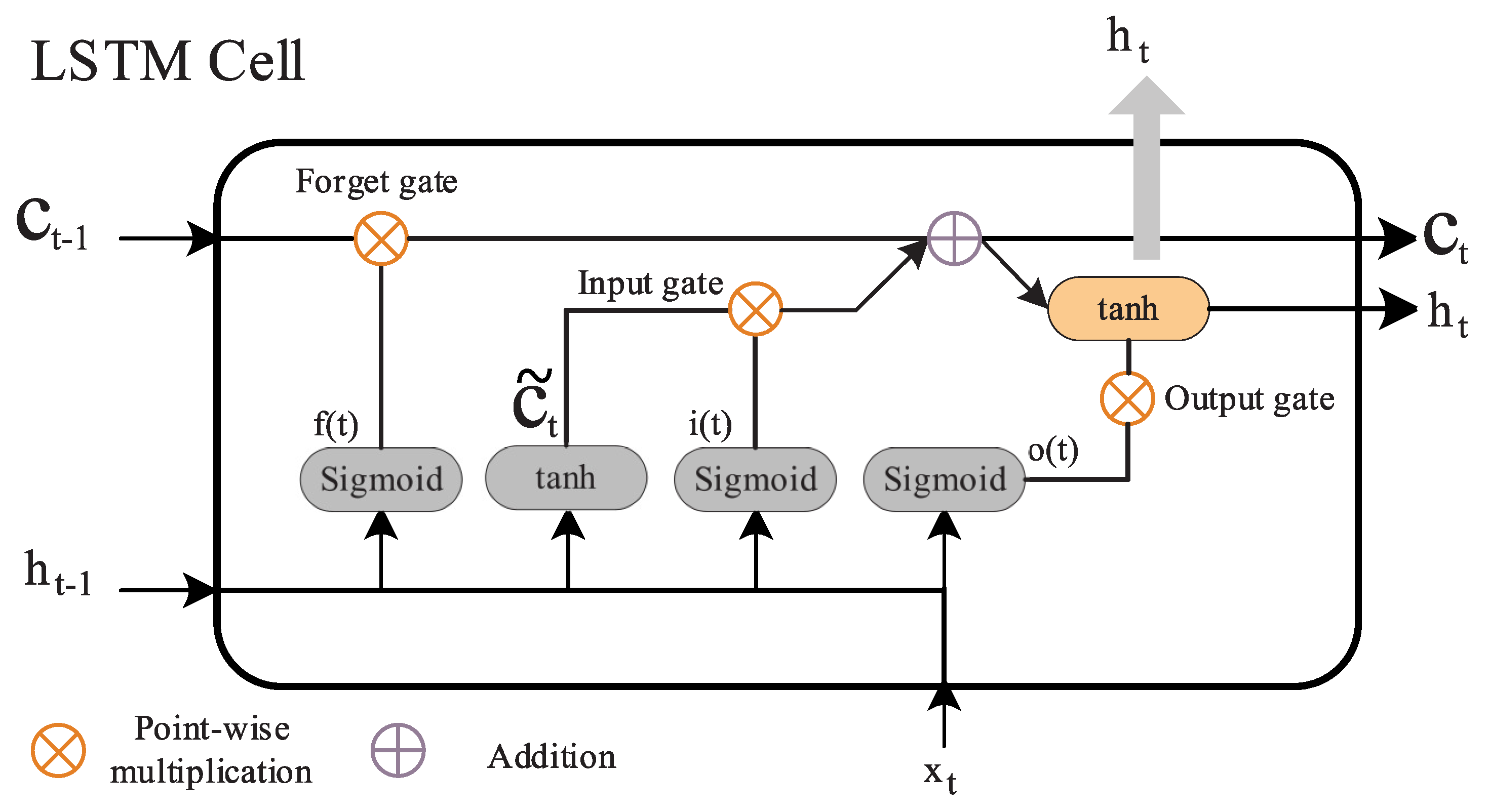
RNNs have the problem of exploding and vanishing gradient when learning long dependencies. The LSTM network model solves this issue. An LSTM network consists of a RNN modified to include a cell, with an input gate, output gate, and forget gate [33], so that a LSTM layer is able to learn long-term dependencies, which is useful for time series prediction. The LSTM cell is presented in Figure 8. First, and are used as input of a sigmoidal layer known as “forget gate” in Equation (7), which filters out which information is retained from a previous state. The forget gate returns a vector , where a value of 1 represents “completely use this information” while a 0 represents “completely get rid of this information”. Second, in the “input gate” in Equation (8), which is also a sigmoidal layer, is decided which state values will be updated. Also, a layer generates a candidate , which will update . Both layers output are multiplied to create an update of the state. The state is then updated, discarding the non relevant information and adding the state update, . Finally, the output is generated according the present state in Equation (9). The sigmoidal layer know as “output gate” decides at which states values will conform to the output.
In summary, the key of the LSTM networks is their internal state, which is updated to know what to remember from previous steps, how to update and which are the relevant values for the output. In practice, these significantly improve the results of traditional recurrent neuronal networks for time series analysis. This justifies its use to try to predict the levels of deforestation in the Amazon jungle in the coming years, together with the dense network for the static data.
3. Results
3.1. Data Pre-Processing and Augmentation
According to the algorithm used to develop a Machine Learning model, an adequate pre-processing of the data is required so that the learning algorithm works correctly. In this case, given that there are two different data typologies, they must be structured differently so that they serve as input to the different networks of them that make up the model. In order for a MLP to be able to interpret data correctly, these must be numerical, i.e., categorical variables must be transformed into numerical ones. Furthermore, the data must be transformed to change the values of the features in the data-set to a common scale, without distorting differences in the ranges of values. First, we used two subsets of data: one for fixed variables and one for annual deforestation. Both can be related by the index of the data-frame or by the name of the municipality. Each is treated differently:
- Static data (input of the MLP):
- –
- One Hot Encoding of the “State” variable. The State variable is transformed to a binary vector of the same size as the set of states, where a 1 is used for the belonging state and 0 otherwise.
- –
- Min-max scaling: to assign the numeric variables a value between 0 and 1.
- –
- Each static instance is an array of size 760 × 14: 760 municipalities with their respective variables “Latitude”, “Longitude”, “Total area”, “Non-forest area”, “Hydrography” and 9 possible states (PA, MA, TO, RO, AP, MT, AM, AC, RR).
- Temporal data (input of the LSTM network):
- –
- Min-max scaling: to assign the numeric temporal variables a value between 0 and 1.
- –
- The temporal instances values are of size 760 × 6 × window_size-1: 760 municipalities with their respective variables “Deforestation increment”, “Cumulative deforestation”, “Forest area”, “Cloud cover”, “Not observed”, “Check” for window_size-1 years.
- –
- The label Y: the values of “Deforestation increment”, which is the variable to predict, in the window_size year. This will serve to contrast the output of the model with the real values, with the purpose of using supervised learning in the training of the model.
Data Augmentation
One possible solution is to generate “synthetic” data that replicates the distribution of the real data. This technique is known as data augmentation. With this objective in mind, “replicas” of the municipalities with spurious data are generated. These are real data to which noise has been added, e.g. variations with respect to the real municipalities, so that they are not exact copies and the model is able to generalize correctly. The number of “replicas” to create for each municipality is defined with the number of replicas parameter. Noise is randomly set for the following variables in the following ranges:
- Latitude, Longitude: ±10% of the standard deviation.
- Length: ±10% of the standard deviation.
- Total area: ±30% of the total area, this allows a greater variation in the area to create a sample with small and large municipalities.
- No forest: the proportion with respect to the total area is maintained ±10%.
- Hydrography: the proportion with respect to the total area is maintained ±10%.
- Deforestation increment: the proportion with respect to the total area is maintained ±5%, with this the rest of the temporary variables can be calculated.
In this way, new municipalities are artificially created, which are in the same state (noise is not added to the variable “State”) and are geographically located in a nearby area. The area can vary more to generate municipalities of varied sizes, but maintaining similar proportions of water and non-forest, as well as deforestation throughout the years. Figure 9b shows the new geographical distribution of the augmented data for a number of municipalities with replicas, i.e., 8360 municipalities. This is a higher density of municipalities if one compares with the observed number of municipalities in Figure 9a. For replicas, the data augmentation goes from having 760 municipalities to 8360 (760 actual municipalities plus 10 “replicas” of the actual data). A number of a maximum of replicas, equivalent to 15,960 municipalities, is used to generate the augmented data.
3.2. Model Hyper-Parameter Optimization
Hyper-parameter optimization is the process of choosing a set of optimal hyper-parameters for the selected learning algorithm for the problem being modeled (dataset). A hyper-parameter is a parameter whose value is used to control the learning process. For the presented model the hyper-parameters have been discussed in the Section 2: Hybrid learning model. The hyper-parameters to be optimized are listed as follows:
- Window size: LSTM temporal window size of the input to model the temporal output.
- Number of municipalities: augmented data, according the number of replicas .
- Batch size: number of samples processed before the model is updated.
- Hidden layers: Hidden layers in the MLP.
Figure 10 shows the results of the hyper-parameter optimization. The best hyper-parameter combination corresponds to the one resulting in a model with minimum mean square error MSE. Figure 10a depicts the minimum MSE for a combination of a window size of 5 years (orange dashed curve) with replicas, that is 15,960 municipalities in the augmented data. Figure 10a depicts that the minimum MSE is achieved for a combination of 2 hidden layers and a batch size of 32 samples. Summarizing the best model is obtained for a LSTM window size of 5 years, 15,960 municipalities for the augmented data, 2 hidden layers and a batch size of 32 samples for the MLP static model.
The loss of the base model built using the original data is compared with the loss of the optimized model (optimized hyper-parameters), can be observed in Figure 11. The loss function corresponds to the cross-entropy, which is a common loss function in machine learning when optimizing neural networks [34,35]. The base model is trained with 760 municipalities during 100 epochs. One can observe that over-fitting takes place from approximately 20 epochs onwards, where the loss in the training set (unseen data) increases, as illustrated in Figure 11a. Over-fitting is an indication that the model learns very specific details of the training set, losing the ability to generalize its predictions to new inputs from unseen data. The model loss for the optimized hyper-parameter combination discussed before is presented in Figure 11a. The loss in the test set does not indicate over-fitting compared with the base model trained only with 760 municipalities. In the loss curve of the best model, it is possible to appreciate continuous learning until step 30. From there the error starts to increase suggesting to stop the training on early stage of the learning epochs. Thus, one can conclude that the optimized model is fit to model the deforestation increment for the original dataset and predict the deforestation for the next decade.
3.3. Model Performance
The regression model obtained from the hyper-parameter optimization process can be tested to measure its prediction performance. The observed data in year 2020 for all 760 municipalities, will be compared with the predicted output of the model for the same municipalities. Note that the model is built on replicas of augmented data, and will be tested on the original data corresponding to the 760 municipalities. Each municipality have a unique index, to identify the original data from the augmented data where the unique index is also coded with the corresponding number of replica index + . The difference between observed y and predicted data values (by the model) are known as residuals in a statistical or machine learning model. They are a diagnostic tool for evaluating the quality of a model. Residuals are also known as errors, and can be defined as [36]. A residual or error analysis will be carried out for each of the 760 municipalities for the year 2020, and the model predicted output.
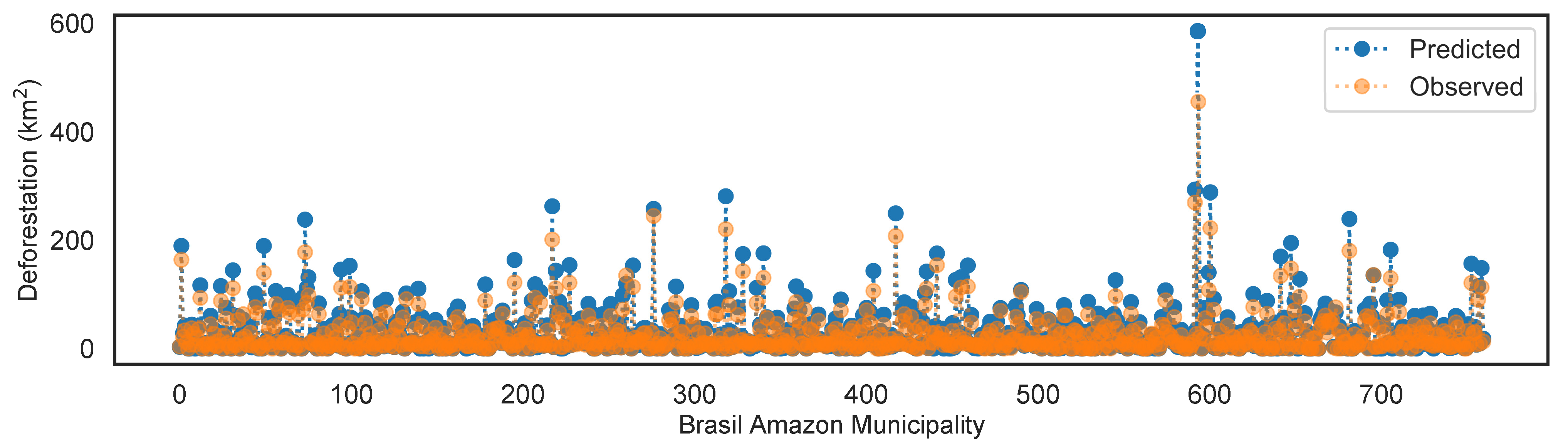
Figure 12 depicts a comparison of the Predicted value (blue dots) vs. the Observed actual value (orange dots) for the 760 Brazil Amazon municipalities deforestation in km. It can be appreciated that both predicted and observed values are very close, indicating that the error is generally small. The more the difference between the blue and orange dots, the larger the error of the predicted value by the model. Also, can be appreciated that the model is overestimating the predicted value, i.e., the predicted values (blue dots) are higher than the observed values (orange dots).
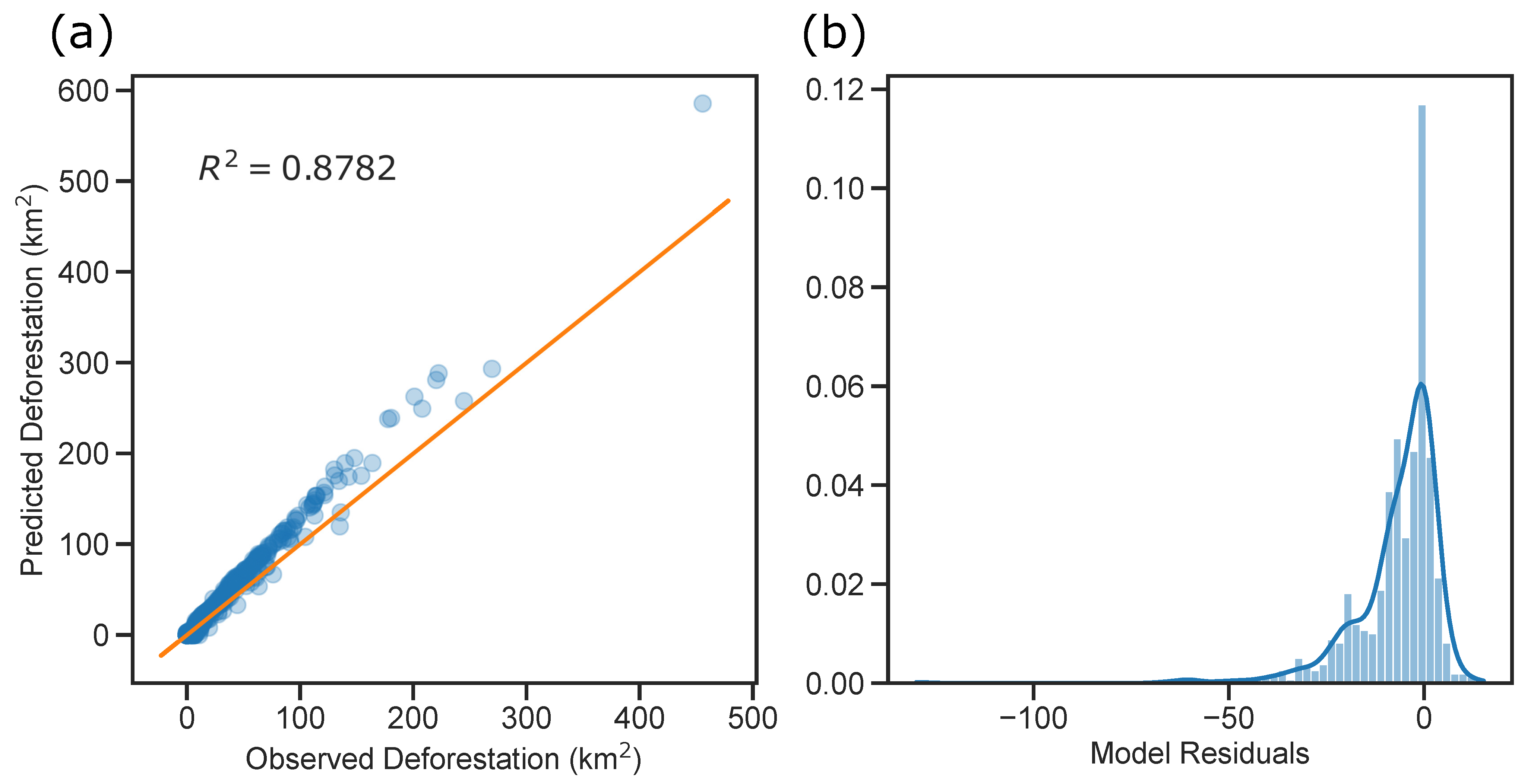
The residual analysis can be visualized, also, using the scatter plot in Figure 13a. The Observed (actual values) of the Deforestation for each of the 760 municipalities is depicted in the x-axis, while the y-axis depicts the deforestation value predicted by the model. The orange line represents the 1:1 line, where a dot will lie, if the predicted value is exactly equal to the observed one. Thus, the orange line represents the perfect regression (no prediction error), where the residual is equal to zero. The closer a point is to the orange line, the better is the prediction. It can be appreciated, that most of the points fall above the orange line, this corresponds to a higher positive slope indicating a steeper upward tilt when compared to the orange line used as reference. As aforementioned, this shows that the model is overestimating the deforestation value, i.e., the predicted value is larger than the observed one. However, in general, the points are close to the orange line, indicating a good prediction performance. Besides the visual analysis performed, the R-squared score, Mean Absolute Error (MAE), and Root Mean Square Error (RMSE), can be used to asses quantitatively the quality of the prediction performed by the regression model [36]. The R-squared can be defined as , , where , and , where is the mean of the observed values. That is, , indicates the proportion of the variation in the dependent variable that is predictable from the independent variables, for the regression model. For the optimized hybrid learning model the R-squared score is , indicating that the regression model accounts for 87.82% of the variance. Such high value for the , indicates a good prediction quality for the 760 municipalities in the dataset.
The residuals (errors) of the model are plotted in Figure 13b. The residual or error for each of the municipalities can be calculated subtracting the Observed value from the predicted value (). A histogram of the residuals is plotted in Figure 13b with a density plot overlaying the histogram. It can be observed that most of the residuals (≈69%) are negative, indicating that the predicted value is higher than the observed one, i.e., the model is overestimating the actual value. However, in average this overestimation is small (close to zero), with a mean value of the residuals of −6.8174 km. In the histogram, outliers can be appreciated, where the occurrence of a single (one) residual larger than |100 km is present. The residuals have a minimum of −130.022355, with the following quartiles, Q1 (25%) of −9.679812 Q2 (50%) of −3.280831 Q3 (75%) of 0.000000 and a maximum of 15.260053. Then, the 50% of the mid residuals (between Q1 and Q3) are between than −9.679812 km and 0 km, which can be considered a good prediction. From the residuals, the quality of the model predictions can be assessed, calculating the mean absolute error, MAE, from the absolute values of the . The MAE of the model is of MAE = 7.83 km, indicating that the absolute error for any of the municipalities predicted deforestation is of 7.83 km in average. Finally, the mean square error, MSE, can be calculated from the square residuals . The root of the , indicates that in average the root mean square error for any of the 760 municipalities is of of 13.24 km. This, measures indicate the quality of the prediction returned by the model, which can be considered good for the present problem. In the following subsection the prediction for all 760 municipalities, is summarized for each year from 2020 to 2030, forecasting the next decade of deforestation increase in the Brazilian Amazon rain-forest.
3.4. Deforestation Forecasting
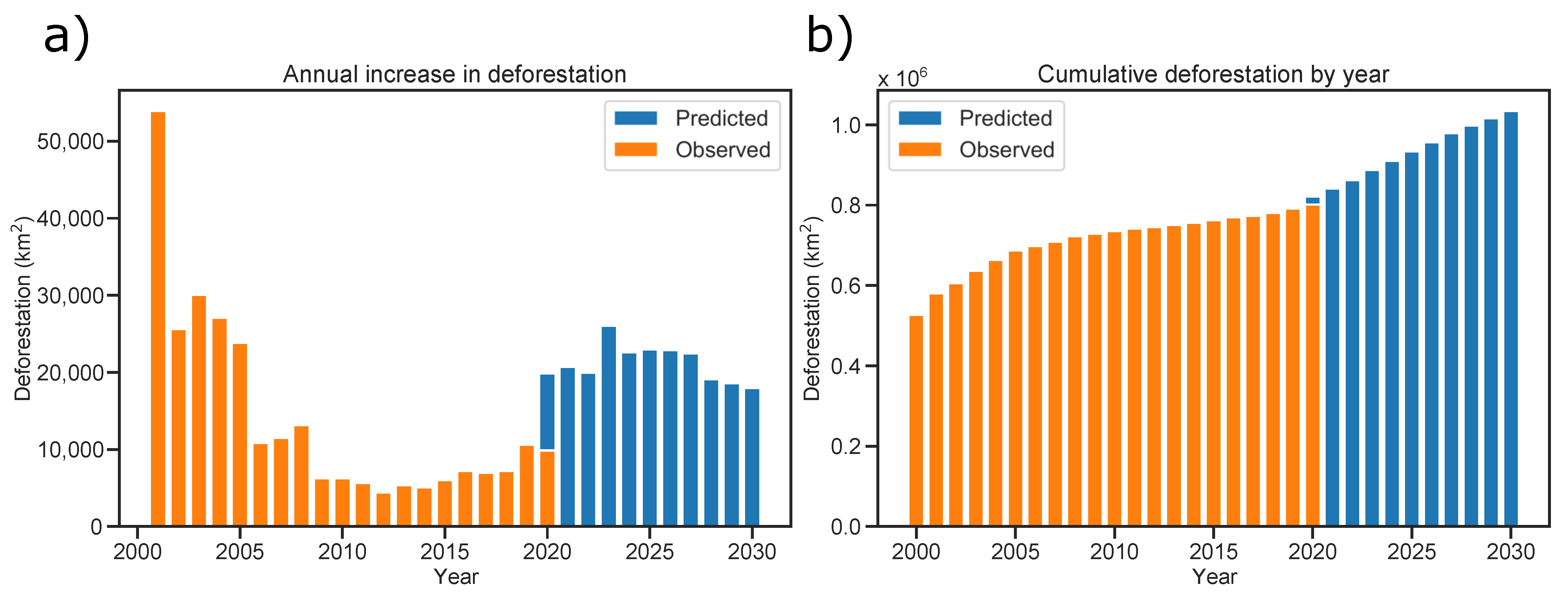
The yearly forecast from 2020 to 2030 is shown in Figure 14. The prediction of the increment in deforestation has been carried out for all the 760 municipalities until 2030. The resulting prediction has been aggregated, to calculate the total increment of deforestation by year. Figure 14a depicts the observed deforestation increase from 2000–2020 in orange bars, the blue bars represent the forecast from 2020–2030. Year 2020 is an overlap, comparing observed versus predicted deforestation for that single year. Similarly, Figure 14a shows the cumulative deforestation, again, observed is presented in orange bars, and predicted in blue bars with the 2020 year overlap. The observed and forecasted data are summarized in Table 3. In light of the actual data, it can be seen that, after a few years in which deforestation has been reduced, an upward trend is being developed. Figure 14a and Table 3 show that deforestation increases in the 2020s, but there is a maximum in 2023 and from 2025 it decreases slowly. In general, the model predicts a prolongation of the incremental trend in deforestation, observed in the last two years, but at a remarkably greater pace for the next decade. It may be that the deforestation in the coming years could have been overestimated by the model, but nevertheless, the model presents a probable scenario where the forest lost pace is worrisome, inviting all of us to take action before it is too late.
4. Discussion and Conclusions
A hybrid learning model was presented to forecast the deforestation increment of the Amazon rain-forest. A dense neural network, namely an MLP, was used to model the geographical static data, together with a LSTM network to model the temporal data of deforestation. A data augmentation process proved to be useful to improve the learning model, as demonstrated in the hyper-parameter optimization, given that the model built on such data performed better. The model proved to be useful to forecast the Amazon deforestation in the coming years. After analyzing the results obtained, it is clear that the situation is not ideal and the trend must be reversed to give a hopeful future to the Amazon. The Amazon rain-forest covers between 5.5 and 6.7 millions of square kilometers and from 2008 to 2018 less than 8000 square kilometers have been deforested annually, less than 1% of the forest area. However the Amazon rain-forest continue to decline daily. The most worrying scenario is that in 2019 deforestation has exceeded 10,000 square kilometers, which may have influenced the model to predict this upward trend. The presented model predicts a worrisome scenario where, it is estimated that by 2030 the accumulated deforestation will be 1 million of square kilometers, around 15% of the actual forest. As stated in the results, probably the model has overestimated the deforestation increase for the next decade, but it is not an impossible scenario. As the hypothesis of this work proposes, a proper data augmentation from 20 years data, and a model hyper-parameter optimization was carefully performed, to avoid over-fitting. Forecasting is always a complex task, but we are confident that the present model predicts a likely scenario, and invite us all to take action.
The socioeconomic context of Brazil, aggravated by the global pandemic, which is currently the center of attention, may not be the most favorable scenario for taking the pertinent measures to protect the Amazon. In any case, urgent attention must be paid to the problem of deforestation. It is not too late to save the Amazon, but work must begin to define a course of action to plan medium and long term sustainability of the rain-forest. Human beings have been using the resources offered by the planet for centuries to advance and improve the quality of life. In the past, the impact our actions had on the environment was unknown. To this day, this cannot serve as an excuse. Concepts such as climate change, sustainability, or renewable energy are not alien to us. We must be aware that we must take care the planet we temporarily live on, so that future generations will be able to enjoy it as we do today.
This work lays the foundations of a deforestation prediction model for municipalities in the Amazon, combining dense neural and LSTM networks. Over the next few years, we can contrast the results of the predictions and perform retraining to update the model with new data. If new variables become available to the public that can be used, the model will be enriched. In the same way, the data can also be crossed with other sources including socioeconomic variables of the 760 municipalities or the states that were analyzed. Another possible course of action is to develop a new model with another type of data. It would be interesting to have images of the Amazon to accurately identify the annual deforestation. A convolutional neural network could be used to identify in the satellite images, the deforested area from the forest. Thus the present work guarantees a follow up analysis to test its predictive power, as well as to improved the model. It is imperative to become a more sustainable species, this research and related results might help to achieve such goal.
Author Contributions
Conceptualization, D.D. and L.d.J.d.V.; methodology, D.D. and M.G.-R.; software, L.d.J.d.V.; validation, D.D., M.G.-R. and L.d.J.d.V.; formal analysis, D.D. and M.G.-R.; investigation, D.D. and O.P.; data curation, L.d.J.d.V.; writing—original draft preparation, D.D. and L.d.J.d.V.; writing—review and editing, D.D., M.G.-R. and O.P.; visualization, M.G.-R. and O.P.; supervision, D.D. All authors have read and agreed to the published version of the manuscript.
Funding
This research was funded by DGIV-UDLA grant number SIS.MGR.21.01 and by Spanish Ministry of Science grant number PID2020-114867RB-I00.
Institutional Review Board Statement
Not applicable.
Informed Consent Statement
Not applicable.
Data Availability Statement
The data is available in the TerraBrasilis web portal, which is a platform developed by INPE to provide access, query, analysis and dissemination of spatial data generated by government environment monitoring programs. The data is licensed under a Creative Commons Attribution-ShareAlike 4.0 International License on the following web link http://terrabrasilis.dpi.inpe.br/en/home-page/, accessed on 1 December 2021.
Conflicts of Interest
The authors declare no conflict of interest. The funders had no role in the design of the study; in the collection, analyses, or interpretation of data; in the writing of the manuscript, or in the decision to publish the results.
Abbreviations
The following abbreviations are used in this manuscript:
| ANN | Artificial Neural Network |
| LSTM | Long-short term memory |
| MLP | Multilayer perceptron |
| RNN | Recurrent Neural Network |
| R | R-squared score |
| MAE | Mean Absolute Error |
| MSE | Mean Squared Error |
| RMSE | Root Mean Squared Error |
| SDGs | Sustainable Development Goals |
References
- Carrasco, L.R.; Le Nghiem, T.P.; Chen, Z.; Barbier, E.B. Unsustainable development pathways caused by tropical deforestation. Sci. Adv. 2017, 3, e1602602. [Google Scholar] [CrossRef] [PubMed] [Green Version]
- Moya-Clemente, I.; Ribes-Giner, G.; Pantoja-Díaz, O. Configurations of sustainable development goals that promote sustainable entrepreneurship over time. Sustain. Dev. 2020, 28, 572–584. [Google Scholar] [CrossRef]
- Miyamoto, M. Poverty reduction saves forests sustainably: Lessons for deforestation policies. World Dev. 2020, 127, 104746. [Google Scholar] [CrossRef]
- United Nations. United Nations Sustainable Development Goal 15. 2018. Available online: https://sdgs.un.org/goals (accessed on 1 December 2021).
- Pacheco, P.; Hospes, O.; Dermawan, A. Zero Deforestation and Low Emissions Development: Public and Private Institutional Arrangements under Jurisdictional Approaches; Center for International Forestry Research: Bogor Regency, Indonesia, 2017. [Google Scholar]
- Mahari, W.A.W.; Azwar, E.; Li, Y.; Wang, Y.; Peng, W.; Ma, N.L.; Yang, H.; Rinklebe, J.; Lam, S.S.; Sonne, C. Deforestation of rainforests requires active use of UN’s Sustainable Development Goals. Sci. Total Environ. 2020, 742, 140681. [Google Scholar] [CrossRef] [PubMed]
- Ruiz-Vásquez, M.; Arias, P.A.; Martínez, J.A.; Espinoza, J.C. Effects of Amazon basin deforestation on regional atmospheric circulation and water vapor transport towards tropical South America. Clim. Dyn. 2020, 54, 4169–4189. [Google Scholar] [CrossRef]
- Farias, M.H.C.S.; BeltrÃo, N.E.S.; Santos, C.A.; Cordeiro, Y.E.M. Impact of rural settlements on the deforestation of the Amazon. Mercator 2018, 17, 1–17. [Google Scholar] [CrossRef]
- Nicholson, S.E. Evolution and current state of our understanding of the role played in the climate system by land surface processes in semi-arid regions. Glob. Planet. Chang. 2015, 133, 201–222. [Google Scholar] [CrossRef] [Green Version]
- Carvalho, W.D.; Mustin, K.; Hilário, R.R.; Vasconcelos, I.M.; Eilers, V.; Fearnside, P.M. Deforestation control in the Brazilian Amazon: A conservation struggle being lost as agreements and regulations are subverted and bypassed. Perspect. Ecol. Conserv. 2019, 17, 122–130. [Google Scholar] [CrossRef]
- Reydon, B.P.; Fernandes, V.B.; Telles, T.S. Land governance as a precondition for decreasing deforestation in the Brazilian Amazon. Land Use Policy 2020, 94, 104313. [Google Scholar] [CrossRef]
- Tole, L. Sources of deforestation in tropical developing countries. Environ. Manag. 1998, 22, 19–33. [Google Scholar] [CrossRef]
- Zemp, D.; Schleussner, C.F.; Barbosa, H.; Rammig, A. Deforestation effects on Amazon forest resilience. Geophys. Res. Lett. 2017, 44, 6182–6190. [Google Scholar] [CrossRef] [Green Version]
- González, M.; del Mar Alonso-Almeida, M.; Avila, C.; Dominguez, D. Modeling sustainability report scoring sequences using an attractor network. Neurocomputing 2015, 168, 1181–1187. [Google Scholar] [CrossRef]
- Che, Z.; Purushotham, S.; Cho, K.; Sontag, D.; Liu, Y. Recurrent neural networks for multivariate time series with missing values. Sci. Rep. 2018, 8, 6085. [Google Scholar] [CrossRef] [Green Version]
- González, M.; del Mar Alonso-Almeida, M.; Dominguez, D. Mapping global sustainability report scoring: A detailed analysis of Europe and Asia. Qual. Quant. 2018, 52, 1041–1055. [Google Scholar] [CrossRef]
- Wang, K.; Li, K.; Zhou, L.; Hu, Y.; Cheng, Z.; Liu, J.; Chen, C. Multiple convolutional neural networks for multivariate time series prediction. Neurocomputing 2019, 360, 107–119. [Google Scholar] [CrossRef]
- Dominguez, D.; Pantoja, O.; Pico, P.; Mateos, M.; del Mar Alonso-Almeida, M.; González, M. Panama Papers’ offshoring network behavior. Heliyon 2020, 6, e04293. [Google Scholar] [CrossRef] [PubMed]
- Liu, Y.; Gong, C.; Yang, L.; Chen, Y. DSTP-RNN: A dual-stage two-phase attention-based recurrent neural network for long-term and multivariate time series prediction. Expert Syst. Appl. 2020, 143, 113082. [Google Scholar] [CrossRef]
- Mayfield, H.J.; Smith, C.; Gallagher, M.; Hockings, M. Considerations for selecting a machine learning technique for predicting deforestation. Environ. Model. Softw. 2020, 131, 104741. [Google Scholar] [CrossRef]
- Jaffé, R.; Nunes, S.; Dos Santos, J.F.; Gastauer, M.; Giannini, T.C.; Nascimento, W., Jr.; Sales, M.; Souza, C.M.; Souza-Filho, P.W.; Fletcher, R.J. Forecasting deforestation in the Brazilian Amazon to prioritize conservation efforts. Environ. Res. Lett. 2021, 16, 084034. [Google Scholar] [CrossRef]
- Ortega Adarme, M.; Queiroz Feitosa, R.; Nigri Happ, P.; Aparecido De Almeida, C.; Rodrigues Gomes, A. Evaluation of deep learning techniques for deforestation detection in the Brazilian Amazon and cerrado biomes from remote sensing imagery. Remote Sens. 2020, 12, 910. [Google Scholar] [CrossRef] [Green Version]
- Lee, S.H.; Han, K.J.; Lee, K.; Lee, K.J.; Oh, K.Y.; Lee, M.J. Classification of Landscape Affected by Deforestation Using High-Resolution Remote Sensing Data and Deep-Learning Techniques. Remote Sens. 2020, 12, 3372. [Google Scholar] [CrossRef]
- Brus, J.; Pechanec, V.; Machar, I. Depiction of uncertainty in the visually interpreted land cover data. Ecol. Inform. 2018, 47, 10–13. [Google Scholar] [CrossRef]
- De Bem, P.P.; de Carvalho Junior, O.A.; Fontes Guimarães, R.; Trancoso Gomes, R.A. Change detection of deforestation in the Brazilian Amazon using landsat data and convolutional neural networks. Remote Sens. 2020, 12, 901. [Google Scholar] [CrossRef] [Green Version]
- Maretto, R.V.; Fonseca, L.M.; Jacobs, N.; Körting, T.S.; Bendini, H.N.; Parente, L.L. Spatio-temporal deep learning approach to map deforestation in amazon rainforest. IEEE Geosci. Remote Sens. Lett. 2020, 18, 771–775. [Google Scholar] [CrossRef]
- Lara-Benítez, P.; Carranza-García, M.; Riquelme, J.C. An Experimental Review on Deep Learning Architectures for Time Series Forecasting. arXiv 2021, arXiv:2103.12057. [Google Scholar] [CrossRef] [PubMed]
- Assis, L.F.; Ferreira, K.R.; Vinhas, L.; Maurano, L.; Almeida, C.; Carvalho, A.; Rodrigues, J.; Maciel, A.; Camargo, C. TerraBrasilis: A spatial data analytics infrastructure for large-scale thematic mapping. ISPRS Int. J. Geo-Inf. 2019, 8, 513. [Google Scholar] [CrossRef] [Green Version]
- Hecht-Nielsen, R. Theory of the backpropagation neural network. In Neural Networks for Perception; Elsevier: Amsterdam, The Netherlands, 1992; pp. 65–93. [Google Scholar]
- Chauvin, Y.; Rumelhart, D.E. Backpropagation: Theory, Architectures, and Applications; Psychology Press: Hove, UK, 2013. [Google Scholar]
- Sibi, P.; Jones, S.A.; Siddarth, P. Analysis of different activation functions using back propagation neural networks. J. Theor. Appl. Inf. Technol. 2013, 47, 1264–1268. [Google Scholar]
- LeCun, Y.; Bengio, Y.; Hinton, G. Deep learning. Nature 2015, 521, 436–444. [Google Scholar] [CrossRef] [PubMed]
- Hochreiter, S. JA1 4 rgen Schmidhuber. “Long Short-Term Memory”. Neural Comput. 1997, 9, 1735–1780. [Google Scholar] [CrossRef] [PubMed]
- Murphy, K.P. Machine Learning: A Probabilistic Perspective; MIT Press: Cambridge, MA, USA, 2012. [Google Scholar]
- Wang, Q.; Ma, Y.; Zhao, K.; Tian, Y. A comprehensive survey of loss functions in machine learning. Ann. Data Sci. 2020, 1–26. [Google Scholar] [CrossRef]
- Fernández-Delgado, M.; Sirsat, M.S.; Cernadas, E.; Alawadi, S.; Barro, S.; Febrero-Bande, M. An extensive experimental survey of regression methods. Neural Netw. 2019, 111, 11–34. [Google Scholar] [CrossRef] [PubMed]
Figure 1.
Research workflow: from raw data to forecasting Amazon deforestation.

Figure 2.
Amazon rain-forest deforestation up to 2020 depicted in yellow. In orange the Brazilian Amazon biomass limits.
Figure 2.
Amazon rain-forest deforestation up to 2020 depicted in yellow. In orange the Brazilian Amazon biomass limits.

Figure 3.
(a) Forest area by State in 2000 and 2020. (b) Rate of forest lost by State. States: Amazon: AM, Roraima: RR, Acre: AC, Rondonia: RO, Mato Groso: MT, Amapá: AP, Pará: PA, Tocatins: TO, Maranhão: MA.
Figure 3.
(a) Forest area by State in 2000 and 2020. (b) Rate of forest lost by State. States: Amazon: AM, Roraima: RR, Acre: AC, Rondonia: RO, Mato Groso: MT, Amapá: AP, Pará: PA, Tocatins: TO, Maranhão: MA.

Figure 4.
(a) Annual increment in deforestation from 2001 to 2020. (b) Cumulative deforestation by year.
Figure 4.
(a) Annual increment in deforestation from 2001 to 2020. (b) Cumulative deforestation by year.

Figure 5.
Schematic representation of the hybrid learning model. Green nodes represent the static input of dense neural network (Multi-layer perceptron). Orange node represent the time series input for the long short term memory (LSTM) model. The regression output (red node) is result of the combined (hybrid) model.

Figure 6.
Schematic representation of a McCulloch-Pitts neuron, which is the base unit of the Multi-layer perceptron.
Figure 6.
Schematic representation of a McCulloch-Pitts neuron, which is the base unit of the Multi-layer perceptron.

Figure 7.
Schematic representation of an LSTM network.

Figure 8.
Schematic representation of an LSTM cell.

Figure 9.
(a) Municipalities in original data-set. (b) Municipalities in augmented data.

Figure 10.
Hyper-parameter optimization: the minimum MSE for each parameter combination is depicted. (a) Different number of municipalities (according the number of replicas in augmented data), and LSTM: Window size. (b) MLP Hidden Layers, Batch size.
Figure 10.
Hyper-parameter optimization: the minimum MSE for each parameter combination is depicted. (a) Different number of municipalities (according the number of replicas in augmented data), and LSTM: Window size. (b) MLP Hidden Layers, Batch size.

Figure 11.
(a) Model loss for the base model parameter combination (no data augmentation). (b) Model loss for best combination of hyper-parameters (with data augmentation).
Figure 11.
(a) Model loss for the base model parameter combination (no data augmentation). (b) Model loss for best combination of hyper-parameters (with data augmentation).

Figure 12.
Predicted (blue dots) versus Observed (blue dots) deforestation for year 2020.

Figure 13.
(a) Observed (x-axis) versus Predicted (y-axis) Deforestation in km. (b) Residuals of the regression model.
Figure 13.
(a) Observed (x-axis) versus Predicted (y-axis) Deforestation in km. (b) Residuals of the regression model.

Figure 14.
(a) Annual increment of deforestation. (b) Cumulative deforestation. Observed deforestation from 2000 to 2020 (orange). Predicted deforestation from 2020 to 2030 (blue).
Figure 14.
(a) Annual increment of deforestation. (b) Cumulative deforestation. Observed deforestation from 2000 to 2020 (orange). Predicted deforestation from 2020 to 2030 (blue).


Table 1.
Data description.
| Static Variables | |||
|---|---|---|---|
| Notation | Variable | Type of Data | Values/Description |
| Municipality | Categorical | Amazon: AM, Roraima: RR, Acre: AC, Rondonia: RO, Mato | |
| Groso: MT, Amapá: AP, Pará: PA, Tocatins: TO, Maranhão: MA. | |||
| Latitude | Numerical | Geographical coordinate | |
| Longitude | Numerical | Geographical coordinate | |
| Total Area | Numerical (km) | Total area of the municipality | |
| Non-forest land area | Numerical (km) | Non-forest land use (i.e., agriculture) | |
| Hydrography area | Numerical (km) | Area covered by rivers and lakes | |
| Temporal Variables | |||
| Notation | Variable | Type of Data | Values/Description |
| Year | Numerical | Temporal index of the data | |
| Deforestation increment | Numerical (km) | Deforestation area that occurred in that year | |
| Cumulative deforestation | Numerical (km) | Total accumulated deforestation area up to that year | |
| Forest area | Numerical (km) | Forest area in that year | |
| Cloud cover | Numerical (km) | Area covered by clouds in that year | |
| Not observed | Numerical (km) | Area not observed in that year | |
| Consistency check | Numerical (km) | Difference between municipality area and all area variables. | |
Table 2.
Rain-forest deforestation by State.
| State | Forest in 2000 (km) | Forest in 2020 (km) | Forest Lost (km) | Percent Lost |
|---|---|---|---|---|
| MT | 371,093.3 | 302,392.35 | 68,700.95 | 18.51 |
| MA | 68,806.3 | 30,346.30 | 38,460.00 | 55.90 |
| AP | 105,764.7 | 87,863.31 | 17,901.39 | 16.93 |
| RR | 156,588.4 | 88,778.64 | 67,809.76 | 43.30 |
| AM | 1,462,388.9 | 1,343,017.65 | 119,371.25 | 8.16 |
| PA | 944,248.1 | 761,848.27 | 182,399.83 | 19.32 |
| RO | 149,807.7 | 117,760.03 | 32,047.67 | 21.39 |
| TO | 10,755.7 | 9975.25 | 780.45 | 7.26 |
| AC | 154,785.5 | 129,185.17 | 25,600.33 | 16.54 |
Table 3.
Rain-forest deforestation by State.
| Year | Deforestation Increment (km) | Cumulative Deforestation (km) |
|---|---|---|
| 2001 | 53,925.0 | 53,925.0 |
| 2002 | 25,607.0 | 79,532.0 |
| 2003 | 30,076.0 | 109,608.0 |
| 2004 | 27,082.0 | 136,690.0 |
| 2005 | 23,852.0 | 160,542.0 |
| 2006 | 10,834.0 | 171,376.0 |
| 2007 | 11,480.0 | 182,856.0 |
| 2008 | 13,173.0 | 196,029.0 |
| 2009 | 6253.0 | 202,282.0 |
| 2010 | 6252.0 | 208,534.0 |
| 2011 | 5659.0 | 214,193.0 |
| 2012 | 4401.0 | 218,594.0 |
| 2013 | 5373.0 | 223,967.0 |
| 2014 | 5100.0 | 229,067.0 |
| 2015 | 6042.0 | 235,109.0 |
| 2016 | 7225.0 | 242,334.0 |
| 2017 | 6955.0 | 249,289.0 |
| 2018 | 7193.0 | 256,482.0 |
| 2019 | 10,608.0 | 267,090.0 |
| 2020 | 9858.0 | 276,948.0 |
| 2020 | 19,852.94 | 19,852.94 |
| 2021 | 20,693.28 | 40,546.22 |
| 2022 | 19,957.98 | 60,504.20 |
| 2023 | 26,050.42 | 86,554.62 |
| 2024 | 22,584.03 | 109,138.65 |
| 2025 | 23,004.20 | 132,142.85 |
| 2026 | 22,899.16 | 155,042.01 |
| 2027 | 22,478.99 | 177,521.00 |
| 2028 | 19,117.65 | 196,638.65 |
| 2029 | 18,592.44 | 215,231.09 |
| 2030 | 17,962.18 | 233,193.27 |
Publisher’s Note: MDPI stays neutral with regard to jurisdictional claims in published maps and institutional affiliations. |
© 2022 by the authors. Licensee MDPI, Basel, Switzerland. This article is an open access article distributed under the terms and conditions of the Creative Commons Attribution (CC BY) license (https://creativecommons.org/licenses/by/4.0/).
Share and Cite
MDPI and ACS Style
Dominguez, D.; del Villar, L.d.J.; Pantoja, O.; González-Rodríguez, M. Forecasting Amazon Rain-Forest Deforestation Using a Hybrid Machine Learning Model. Sustainability 2022, 14, 691. https://0-doi-org.brum.beds.ac.uk/10.3390/su14020691
AMA Style
Dominguez D, del Villar LdJ, Pantoja O, González-Rodríguez M. Forecasting Amazon Rain-Forest Deforestation Using a Hybrid Machine Learning Model. Sustainability. 2022; 14(2):691. https://0-doi-org.brum.beds.ac.uk/10.3390/su14020691
Chicago/Turabian StyleDominguez, David, Luis de Juan del Villar, Odette Pantoja, and Mario González-Rodríguez. 2022. "Forecasting Amazon Rain-Forest Deforestation Using a Hybrid Machine Learning Model" Sustainability 14, no. 2: 691. https://0-doi-org.brum.beds.ac.uk/10.3390/su14020691
Note that from the first issue of 2016, this journal uses article numbers instead of page numbers. See further details here.