Aquila Optimization Based Harmonic Elimination in a Modified H-Bridge Inverter

Abstract

Multilevel inverters (MLIs) are capable of producing high-quality output voltage and handling large amounts of power. This reduces the size of the filter while also simplifying the circuitry. As a result, they have a wide range of applications in industries, particularly in smart grids. The input voltage boosting feature is required to use the MLI with renewable energy. Moreover, many components are required to get higher output voltage levels that add weight and cost to the circuit. Numerous MLI topologies have been identified to minimize the losses, device count, and device ratings. A seven-level modified H-bridge inverter with a reduced component count, and reduced THD is presented in this paper. Two DC sources with six IGBTs have been used to generate a seven-level output voltage, and the Aquila Optimizer (AO) has been implemented to get the regulated output. MATLAB/Simulink environment has been used for designing the simulation model. Furthermore, the simulation result has been validated in the laboratory on a hardware setup using the DSP-TMS320F28335 Launchpad. With the reduced number of switching devices as well as the dc supply, the size of the inverter is compacted and becomes more economical.

1. Introduction

During recent years, multilevel inverters gained popularity in various power electronics and renewable energy applications. It is due to enhanced power quality, reduced filter requirement, high modularity, and reduced device stresses [1]. Drives and grid integration applications rely on inverters for their functioning. The multilevel inverters were proposed to address the shortcomings of the traditional two-level inverter. Although conventional two-level inverters are simple to construct, they have several drawbacks. Their application is limited to a small power range due to high total harmonic distortion (THD), which requires better filter design and higher blocking voltage rating devices to improve power quality. The multilevel inverter produces a multi-stepped ac voltage from multiple dc voltage levels. The flying capacitor, diode clamped, and cascaded H-bridge topologies are the most common multilevel inverter topologies [1,2,3,4]. The flying capacitor MLI and diode clamped MLI suffers from the uneven voltage distribution across the capacitor connected in series. Moreover, in diode clamped MLI, the diode requirement increases with an increase in the levels. For high voltage generation, the number of components also increases. Hence, their use is limited only to low and medium-voltage industrial applications [5,6]. Cascaded H-bridge MLI necessitates the use of multiple isolated dc sources.

In recent years, numerous fascinating topologies, such as topologies implemented with quasi Z-source and transformers, have been proposed to overcome the shortcomings of conventional MLIs [2]. Switched-capacitor using the series-parallel configuration in multilevel inverters is becoming more popular these days [7,8]. H-bridge can be used at the end of multilevel inverters to withstand the high voltage stress. To achieve a compact topology with lower losses, higher total standing voltage, and reduced cost, many topologies based on a smaller number of diodes, power switches, isolated dc sources, and capacitors have been proposed [9,10]. The MLI structure should be typically flexible and modular, with the ability to be cascaded or arranged in such a way to get a boosted and approximate the sinusoidal output voltage with a large number of levels. Voltage boosting is not possible with commercially available multilevel inverters. For converters designed to use in renewable energy systems, voltage boosting capability will be critical because the voltage generated by fuel cells and PV panels is insufficient and must be boosted to use for grid integration [9]. Some MLI topologies have small voltage gain. Moreover, the MLIs have several dc voltage sources. The MLI’s size, cost, and complexity are reduced by reducing the component count [11,12]. Hence, switching capacitors were introduced in MLIs to achieve the above-said objective. As a result, recent research has focused on the Switched Capacitor (SC) MLI, which is a promising voltage booster while using the fewest dc sources only [13]. Switched Capacitor MLIs have inherent voltage boosting capabilities. SCMLIs work on the principle of charging and discharging the capacitor to a certain voltage value using some techniques. While using the capacitor as a substitute for dc power supply, balancing the capacitor voltage is challenging [14,15,16,17].

Different optimization techniques are being used in the area of microgrid and power systems. Authors in [18] proposed a hybrid optimization for microgrids based on a cyber-physical power system (CPPS). In recent years, multilevel inverters (MLI) topologies have been widely adopted in renewable energy system applications due to higher harmonics distortion in conventional inverters [19]. A lot of work has been done on H-bridge multilevel inverters [20]. Controlling the output voltage in an MLI and simultaneously reducing the harmonic content has been an area of research. Different modulation schemes have been proposed for the same. Basically, the schemes can be divided into low and high-frequency modulation schemes. Low-frequency modulation schemes include nearest level control, selective harmonic elimination, selective harmonic mitigation, etc., while high-frequency modulation schemes include phase and level shifted PWM schemes. Low-frequency schemes have the advantage of lower switching loss and consequently higher efficiency.

This work uses the Aquila Optimizer (AO) algorithm to solve the SHE equations in the seven-level modified H-bridge inverter. The AO is a population-based optimization algorithm inspired by Aquila’s natural behavior while grabbing prey [21]. The Aquila are known to use four different hunting strategies, each with its own set of characteristics and the capacity of most Aquila to switch between them rapidly and intelligently. High soar with a vertical stoop, contour flight with brief glide attack, low flight with a slow downward attack, and walking and grabbing prey are those strategies that the Aquila used while hunting. These features were included in the algorithm developed for solving the optimization problems. Since SHE is also an optimization problem, authors have used it to optimize the SHE equations for the seven-level modified H-bridge inverter. The topology taken in this paper is the modified H-bridge inverter, which has reduced switching components and no separate diodes. Consequently, the cost and size of the inverter are reduced. Two dc sources have been used to generate a seven-level output voltage. Output waveforms obtained from the simulation and hardware setup verify the effectiveness of the proposed algorithm.

This paper is divided into six sections. While Section 1 was Introduction, discussion and comparison of the seven-level modified H-bridge multilevel inverter with other well-established topologies is made in Section 2. Aquila Optimizer is explained in Section 3 and its formulation for the SHE problem. The simulation results are given in Section 4. The hardware results are discussed in Section 5, and the conclusion part is presented in Section 6.

2. Seven Level Modified H-Bridge Inverter

Multilevel inverters (MLIs) are extensively employed in renewable energy applications for power conversion due to their attractive features, such as the need for fewer dc sources, less dv/dt stress, and output voltage resembling the sine wave. Cascaded H-bridge inverters have gained special attention because of their symmetrical structure, modularity, and ease of control. The requirement for many dc sources is the major disadvantage of the CHB-MLI. However, cascaded H-bridge multilevel inverters outperform the Neutral point diode clamped and flying capacitors due to their modularity. Nevertheless, this required many dc sources, which resulted in several issues, including increased volume and price.

The H-bridge inverter has been modified by adding one additional battery source to the second leg and two more switches in opposite directions between two legs. Many inverters exist for producing seven-level output.

Table 1. Components count for different single-phase seven-level multilevel inverters.

Inverter Type	DC Source	Capacitor	Clamped Diode	Active Switches	Total Parts Count	Complexity of Control
CHB symmetrical	3	0	0	12	15	Low
CHB asymmetrical	2	0	0	8	10	Low
NPC with voltage control	1	6	10	12	29	Very high
NPC without Voltage control	6	0	10	12	28	Low
FC	1	5	0	12	18	High
Modified H bridge	2	0	0	6	8	Very low

illustrates the comparison of some popular multilevel inverters with the proposed inverter for the component count and the control complexity. It is noteworthy that the proposed converter with self-voltage balancing property has fewer component counts and has no control complexity. There are two possible connections of the battery source to generate the seven levels of output, the series adding and the series-opposing connection. 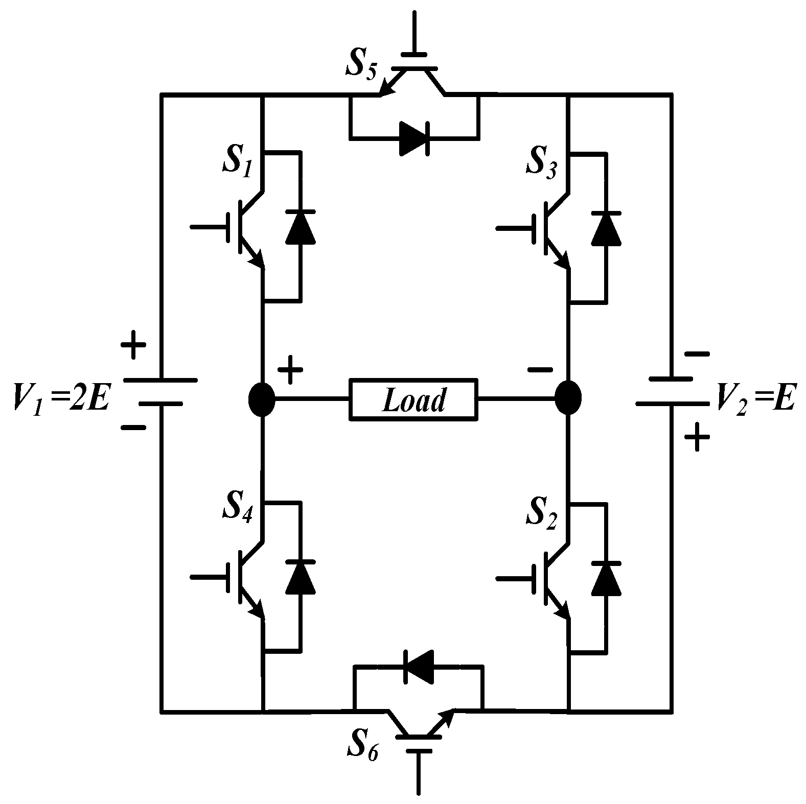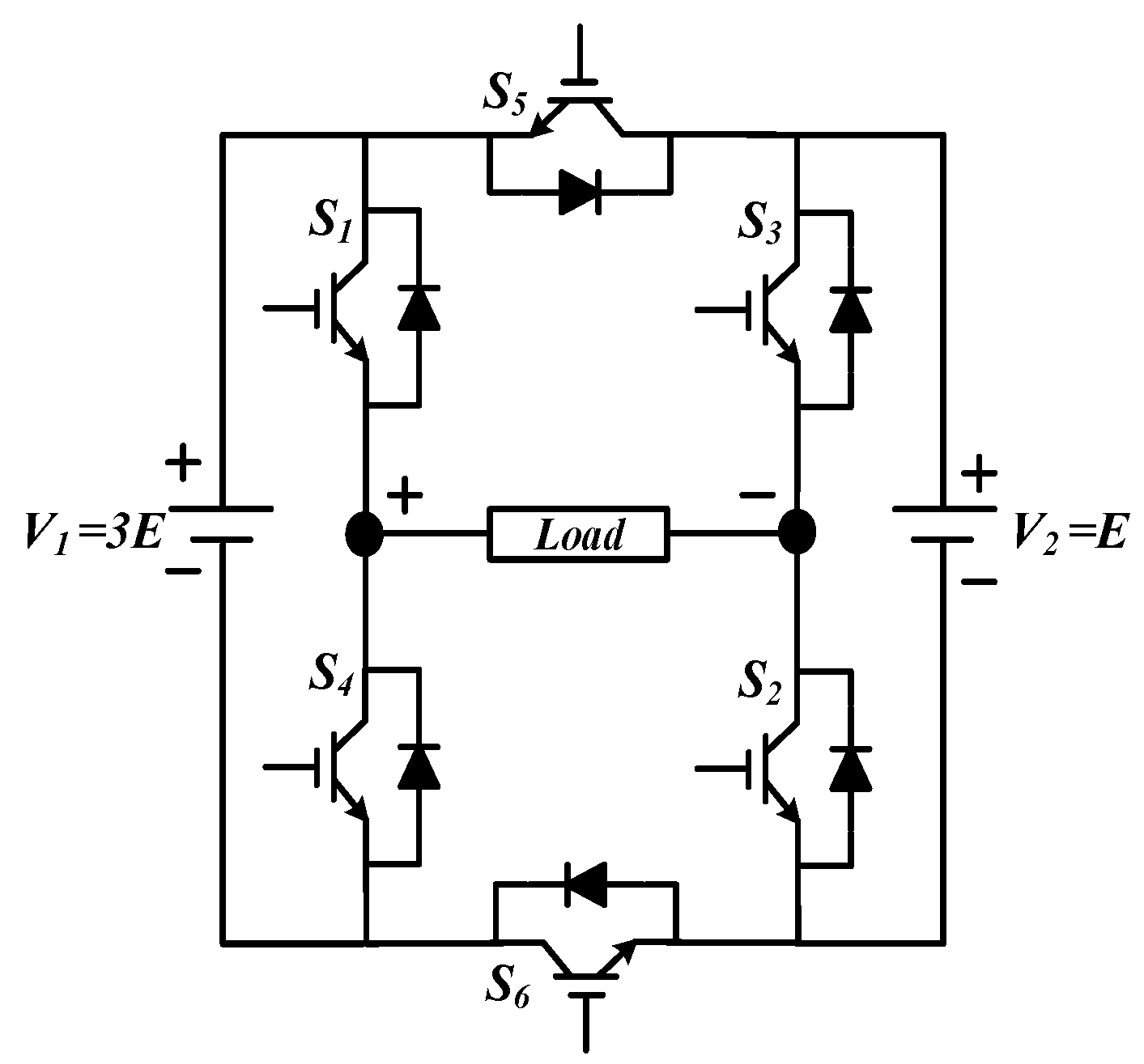Figure 1 shows the series-opposing connection, while Figure 2 shows the series adding.

In the first connection, the maximum output voltage is the addition of both voltage sources. The input voltage ratio is 2:1 to generate the seven equal voltage steps. If the battery V₁ equals 2E and the V₂ equals E, the possible output levels are (0, +E, +2E, +3E and 0, –E, −2E, −3E). If one of the battery sources is replaced by the capacitor, charging is not possible. The input voltage is low as compared to the second connection to obtain the same output voltage. The maximum output voltage equals the higher input voltage source (V1) in the second connection. The input voltage ratio is 3:1 to generate the identical voltage steps. If the input V₁ equals 3E and V₂ equals E, the possible output levels are (0, +E, +2E, +3E and 0, –E, −2E, −3E). The input voltage required is higher as compared to the first connection to obtain the same output voltage. If the battery source (V₂) is replaced with a capacitor, charging is possible due to the same polarity of the battery and the capacitor. The capacitor charges, discharges, and remains unaffected in different switching states. However, the key challenge is balancing the charging and discharging voltage in one complete cycle. If the charging voltage is greater, the capacitor voltage rises until it reaches the battery’s maximum voltage (V1 = V2 = 3E). As a result, it will only generate three levels (0, +3E, and −3E). If discharging is greater in one cycle, the capacitor voltage decreases until it becomes zero. It also generates only three levels, which are (0, +E, and −E). If the capacitor voltage remains constant (E) at the end of the complete cycle after charging and discharging, it can be used instead of the battery to generate the output levels throughout the infinite cycle. The capacitor voltage can be kept constant by using closed-loop voltage control, but it will be very complicated. Moreover, it requires additional circuitry and becomes more expensive and bulkier. Therefore, self-balancing of the capacitor is required to overcome this complexity.

Table 2. Switching states for series adding and opposing connection.

Switching States/Modes	S1	S2	S3	S4	S5	S6	Series Adding	Series Opposing
							Output	Output
I	ON	-	ON	-	ON	-	0	0
II	ON	ON	-	-	ON	-	−(V2) = −E	(V2) = E
III	ON	-	ON	-	-	ON	(V1 + V2) = 3E	(V1 − V2) = 2E
IV	ON	ON	-	-	-	ON	(V1) = 2E	(V1) = 3E
V	-	ON	-	ON	-	ON	0	0
VI	-	-	ON	ON	-	ON	(V2) = E	−(V2) = −E
VII	-	ON	-	ON	ON	-	−(V1 + V2) = −3E	−(V1-V2) = −2E
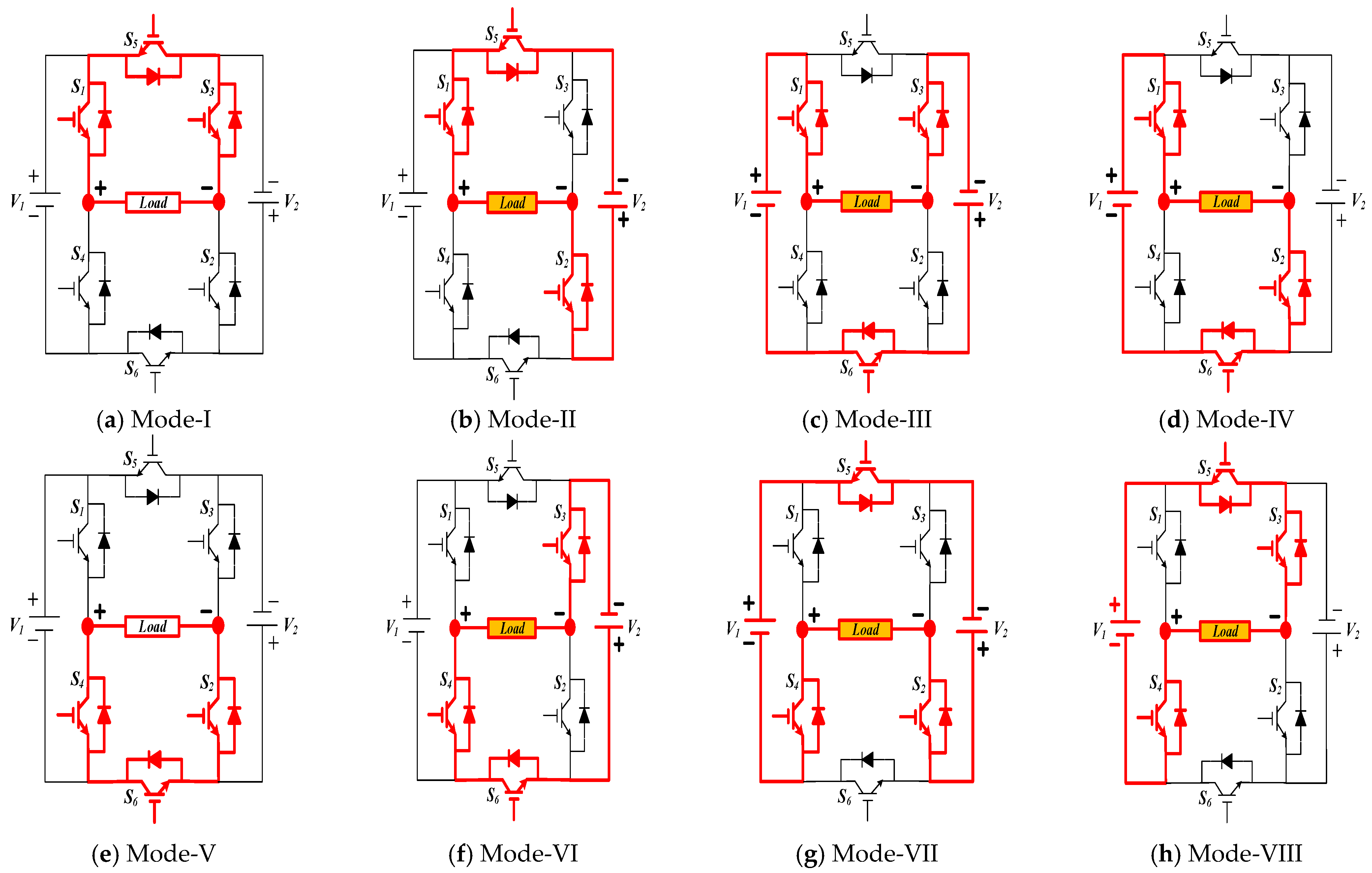
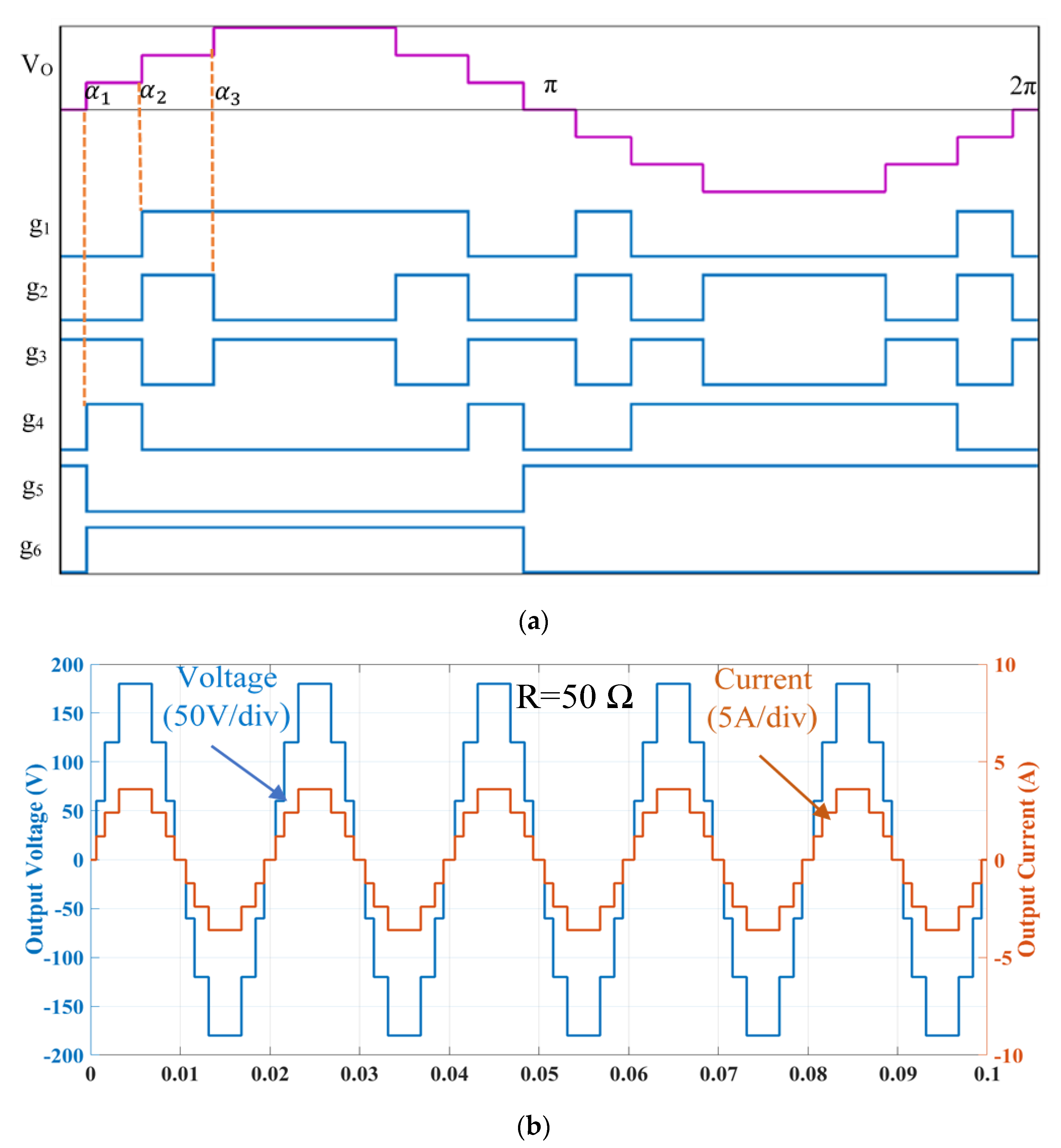
VIII	-	-	ON	ON	ON	-	−(V1) = −2E	−(V1) = −3E

shows the various switching states and possible outputs in both series adding and opposing connections. Figure 3 shows the conduction pattern for the different switching states in series opposing connections.

3. Aquila Optimizer: A Metaheuristic Optimization Algorithm

The Aquila Optimizer (AO) is a population-based optimization algorithm inspired by Aquila’s natural behaviors while grabbing prey [14]. It is one of the most popular birds of prey in the Northern Hemisphere. It is a member of the Accipitridae family, which includes almost all birds. The Aquila are known to use four different hunting strategies, each with its own set of characteristics and the capacity of most Aquila to switch between them rapidly and intelligently.

• For hunting birds in flight, the first method, to high soar with a vertical stoop, is used, in which the Aquila rises high above the ground. The Aquila enters a long, low-angled glide once it has found prey, with speed increasing as the wings shut farther. The Aquila must have a height advantage over its target for this approach to work. To simulate a thunderclap, the wings and tail are unfolded just before the engagement, and the feet are propelled forward to seize the prey.
• The second approach, the contour flight with brief glide attack, is considered as Aquila’s most commonly employed method, in which the Aquila rises from the ground at a low level. Whether the prey is running or flying, the prey is pursued carefully. This strategy is ideal for hunting ground squirrels, breeding grouse, or seabirds.
• A low flight with a slow downward attack is the third method. In this case, the Aquila dives to the ground and then attacks the prey one by one. The Aquila chooses its target and lands on its neck and back, attempting to enter. This approach is used for hunting slow prey like rattlesnakes, hedgehogs, foxes, and tortoises, as well as any species that lacks an escape response.
• Walking and grabbing prey is the fourth approach, in which the Aquila wanders on land and tries to draw its prey. It is used to remove the young of large prey animals (such as deer or sheep) from the covered area.

Finally, Aquila is one of the most clever and skilled hunters, second only to humans. The methodologies listed above served as the main motivation for the suggested AO algorithm. The subsections that follow discuss how the AO models these processes.

3.1. Initialization of the Solution

The optimization rule in AO starts with the generation of a population of candidate solutions (S) as shown in Equation (1), which is created stochastically between the problem’s upper (UB) and lower (LB) bounds. In each iteration, the best-obtained answer is roughly determined as the optimal solution.

$$S=\left[\begin{array}{ccc}\begin{array}{c}{S}_{1,1}\\ S_{1,2}\end{array}& \cdots & \begin{array}{c}\begin{array}{ccc} S_{1,j}& S_{1,m-1}& S_{1,m}\end{array}\\ \begin{array}{ccc} S_{2,j}& \cdots & S_{2,m}\end{array}\end{array}\\ ⋮& \ddots & \begin{array}{ccc}\dots & \dots & \dots \end{array}\\ \begin{array}{c}{S}_{N-1,1}\\ S_{N,1}\end{array}& \cdots & \begin{array}{ccc}\begin{array}{c} S_{N-1,j}\\ S_{N,j}\end{array}& \begin{array}{c} ⋮\\ S_{N, m-1}\end{array}& \begin{array}{c} S_{N-1,m}\\ S_{N,m}\end{array}\end{array}\end{array}\right]$$

(1)

where S signifies a set of current candidate solutions produced at random using Equation (2), S_i denotes the ith solution’s decision values (positions), N denotes the total number of candidate solutions (population), and m denotes the problem’s dimension size.

$$S_{i,j}=rand\times \left(U{B}_j-L{B}_j\right)+L{B}_j, i=1,2,\dots ,\mathrm{N} j=1,2,\dots ,\mathrm{m}$$

(2)

where rand is the random number,$U{B}_j$ denotes jth upper bound, $L{B}_j$ denotes the jth lower bound of the given problem.

3.2. Mathematical Modeling of AO

The suggested AO technique simulates Aquila’s hunting behavior, displaying each phase of the hunt. As a result, the suggested AO algorithm’s optimization processes are divided into four categories: high soar with a vertical stoop, contour flying with short glide attack, exploitation inside a converging search space by low flight with slow descent assault, and swooping by walk and grab prey. The AO algorithm can move from exploration steps to exploitation steps utilizing its various behaviors. If t ≤ (2/3*T), exploration steps are executed; otherwise, the exploitation steps are completed. The mathematical model of AO is as follows:

3.2.1. Expanded Exploitation ($S_1$)

The Aquila recognizes the prey area and chooses the ideal hunting area using the first method ($S_1$), which involves a high soar with a vertical stoop. The AO explores the search arena from a high altitude to determine the location of the prey. This behavior is represented mathematically as Equation (3).

$$S_1\left(t+1\right)=S_{best}\left(t\right)\times \left(1-\frac{t}{T}\right)+\left(S_M\left(t\right)-S_{best}\left(t\right)*rand\right)$$

(3)

where $S_1\left(t+1\right)$ is the solution obtained by the first search procedure $S_1$ for the next iteration of t. The best-obtained solution till the tth iteration is $S_{best}\left(t\right)$, which represents the approximate location of the prey. The term ($1-\frac{t}{T}$) is used to control the number of iterations in the expanded search (exploration). The location mean value of the current solutions connected at the tth iteration is denoted by$S_M\left(t\right)$, which is derived using Equation (4). ‘t’ and ‘T’ represent the current iteration and the maximum number of iterations, respectively. ‘rand’ is a random value between 0 and 1.

$$S_M\left(t\right)=\frac{1}{N}{{\displaystyle \sum }}_{i=1}^N{S}_i\left(t\right), Ɐ\mathrm{j}=1,2,\dots ,\mathrm{m}$$

(4)

where N is the population size and m is the dimension size of the problem.

3.2.2. Narrowed Exploitation ($S_2$)

The Aquila circles over the target prey, prepares the land, and then attacks in the second method ($S_2$). Contour flying with a short glide attack is the name given to this technique. In preparation for the attack, AO narrowly investigates the intended prey’s chosen region. The mathematical expression for this behavior is given in Equation (5).

$$S_2\left(t+1\right)=S_{best}\left(t\right)\times Levy\left(dm\right)+S_R\left(t\right)+\left(y-x\right)*rand$$

(5)

where $S_2\left(t+1\right)$ is the result of the second search method’s next iteration of t. The dimension space is dm, and the levy flight distribution function is Levy(dm), which is derived using Equation (6). At the ith iteration, $S_R\left(t\right)$ is a random solution picked in the range of [1 N].

$$Levy\left(dm\right)=a\times \frac{b\times \sigma }{{\left|c\right|}^{\frac{1}{\beta }}}$$

(6)

where a is constant with a value of 0.01, b and c are random numbers between 0 and 1. $\sigma$ is obtained using Equation (7).

$$\sigma =\left(\frac{\Gamma \left(1+\beta \right)\times \sin \left(\frac{\pi \beta }{2}\right)}{\Gamma \left(\frac{1+\beta }{2}\right)\times \beta \times 2^{\frac{\beta -1}{2}}}\right)$$

(7)

where $\beta$ is a constant with a fixed value of 1.5. In Equation (5), the spiral shape in the search is represented by y and x, which are determined as follows.

$$y=r\times \cos \left(\theta \right)$$

(8)

$$x=r\times \sin \left(\theta \right)$$

(9)

where,

$$r=r_1+W\times d_1$$

(10)

$$\theta =-\alpha \times d_1+{\theta }_1$$

(11)

$${\theta }_1=\frac{3\pi }{2}$$

(12)

$r_1$ has a value between 1 and 20 for a specific number of search cycles, and $W$ is constant with a small value of 0.00565. ‘$d_1$’ is integer values between 1 and the length of the search space (m), $\alpha$ is a small constant term with a value of 0.005.

3.2.3. Expanded Exploitation ($S_3$)

When the prey location is precisely identified and the Aquila is ready to land and strike, the third approach ($S_3$) is used. The Aquila descends vertically with a preliminary attack to detect the prey reaction. Low flying with gradual descent assault is the name of this technique. AO uses the target’s specified area to go close to the prey and attack. Mathematically this behavior can be expressed as in Equation (13).

$$S_3\left(t+1\right)=(S_{best}\left(t\right)-S_M\left(t\right))\times \gamma -rand+\left(\left(UB-LB\right)\times rand+LB\right)\times \delta$$

(13)

where $S_3\left(t+1\right)$ is the solution of the third search method’s next iteration of t. $S_{best}\left(t\right)$signifies the prey’s approximate location till the ith iteration (the best-obtained solution), while$S_M\left(t\right)$ denotes the current solution’s mean value at the tth iteration, which is determined using Equation (4). Here, the exploitation adjustment parameters are set to a small value (0.1). The lower bound of the given problem is denoted by LB, and the upper bound is denoted by UB.

3.2.4. Narrowed Exploitation ($S_4$)

When the Aquila approaches the prey in the fourth method ($S_4$), the Aquila attacks the prey over land based on their stochastic motions. This technique is known as “walk and grab prey”. Finally, in the last spot, AO attacks the prey. Mathematically, this behavior can be expressed as in Equation (14).

$$S_4\left(t+1\right)=Qf\times S_{best}\left(t\right)-\left(P_1\times S\left(t\right)\times rand\right)-P_{2}Levy\left(dm\right)+rand\times P_1$$

(14)

where $S_4\left(t+1\right)$ is the solution of the fourth search method for the following iteration of t. The quality function Qf is used to balance the search techniques and is determined using Equation (15). $P_1$ represents multiple AO motions that are utilized to monitor the prey during the flight and are formed using Equation (16). $P_2$ shows decreasing values from 2 to 0, which represent the AO’s flight slope as it follows the prey during the trip from the first (1) to the last (t) location, which is calculated using Equation (17). The current solution at the tth iteration is $S\left(t\right).$

$$Qf\left(t\right)=t^{\frac{2\times rand-1}{{\left(1-T\right)}^2}}$$

(15)

$$P_1=2\times rand-1$$

(16)

$$P_2=2\times \left(1-\frac{t}{T}\right)$$

(17)

$Qf\left(t\right)$ represents the quality function value for the tth iteration. A flowchart of the Aquila algorithm has been presented in Figure 4.

3.2.5. Selective Harmonic Elimination using Aquila Optimizer

The selective harmonic problem can be developed using the following equations

$$H_1=\frac{3V_{dc}}{\pi }\left[\cos ({\mathsf{\alpha }}_1)+\cos \left({\mathsf{\alpha }}_2\right)+\cos ({\mathsf{\alpha }}_3)\right]$$

(18)

$$H_5=\frac{3V_{dc}}{5\pi }\left[\cos (5{\mathsf{\alpha }}_1)+\cos \left(5{\mathsf{\alpha }}_2\right)+\cos (5{\mathsf{\alpha }}_3)\right]$$

(19)

$$H_7=\frac{3V_{dc}}{7\pi }\left[\cos (7{\mathsf{\alpha }}_1)+\cos \left(7{\mathsf{\alpha }}_2\right)+\cos (7{\mathsf{\alpha }}_3)\right]$$

(20)

H_i represents the magnitude of the various harmonics in the output voltage. In order to incorporate the THD minimization along with the harmonic elimination following objective function is taken.

$$Obj={\left(100\frac{V_{dc}-H_1}{V_{dc}}\right)}^4+{{\displaystyle \sum }}_1^2\frac{{\left(50H_i\right)}^2}{H_1}$$

(21)

where V_dc is the dc source voltage, H₁ represents the fundamental voltage, H_i represents the Fourier equations. The following constraint should also be included in the problem formulation:

0 < α₁ < α₂ < α₃ < π/2

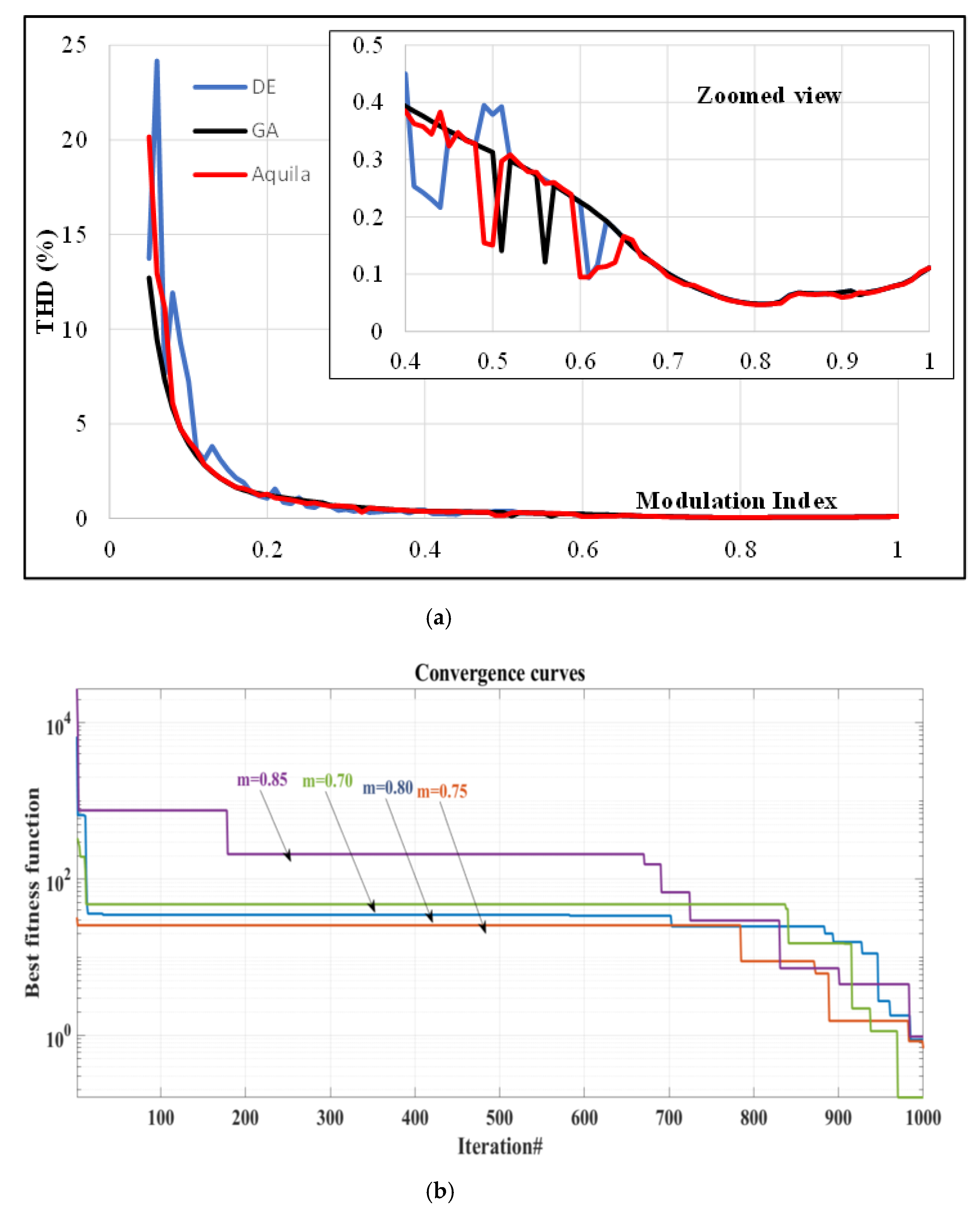
Figure 5a shows the plot between THD per unit and the modulation index for the Aquila optimizer as well as the Genetic algorithm and Differential evolution for the objective function mentioned in Equation (21). Zoomed view for modulation index above 0.4 has also been shown for better view. Aquila optimizer is comparable to both of them and works better in the region where MI is around 0.6, 0.5, and less than 0.2. Figure 5b represents the convergence curve for the Aquila optimizer for four different modulation indices. The number of iterations taken is 1000. The parameters that have been taken in running the optimization code are shown in

Table 3. Parameters used.

Sl. No.	Genetic Algorithm	Differential Evolution	Aquila Optimizer
1	Population = 40	Population = 40	Population = 40
2	Mutation Rate = 0.01	Mutant Factor = 0.01	Alpha = 0.1, delta = 0.1, omega = 0.005
3	Crossover Rate = 0.6	Crossover Rate = 0.6	U = 0.0265, r0 = 10

.

4. Simulation Results

The simulation of the modified H-Bridge inverter has been done in MATLAB^®/Simulink. The two unequal voltage sources (V₁ = 120 V, V₂ = 60 V) have been used to produce different voltage levels. The voltage source is in a 2:1 ratio, which produces a seven-level output voltage. IGBTs have been used for the switches, and the pulse generator block has generated the switching pulse. The simulation parameters are noted in

Table 4. Simulation Parameters.

S. No.	Parameters/Components	Specifications	No. of Components
1.	Voltage Source (DC)	60 V, 120 V	Two
2.	Reference signal frequency	50 Hz	One
3.	Insulated-Gate Bipolar Transistor (IGBT)	Resistance (Internal) = 110−3 Ω Resistance (Snubber) = 110−5 Ω Capacitance (Snubber) Cs = 0	Six
4.	Load	R = 50 Ω, 100 Ω, L = 100 mH	One

. Simulation results have been shown in Figure 6. The different gating signals have been shown in Figure 6a. Figure 6b shows the output voltage and output current waveform for a resistive load of 50 ohms. Output voltage and current waveforms for an inductive load of R = 50 ohms and L = 120 mH have been shown in Figure 6c. Figure 6d, e show the output waveforms for a dynamic load change from a load of 100 ohms to 50 ohms and from 50 ohms to 100 ohms, respectively.

5. Experimental Validation

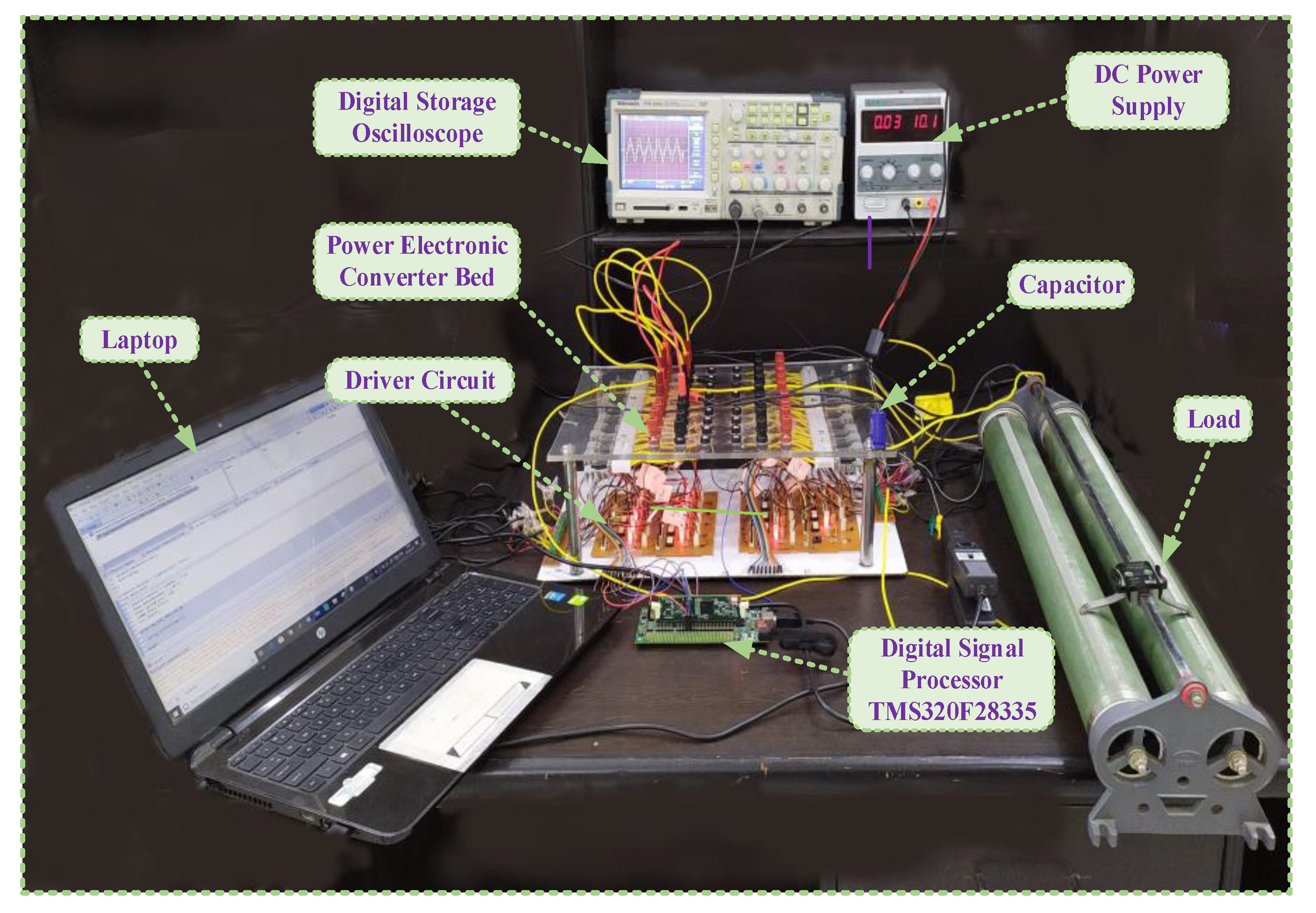
The hardware implementation of the seven-level modified H-bridge has been carried out to validate the proposed topology, which is shown in Figure 7. Six IGBTs (FGA25N120) of 1200 V and 25 A have been used in the setup. TLP-250 Optocoupler is used for the gate driver circuit. Digital signal controller TMS320F28335 (Texas Instruments) has been used to generate the control signal for the IGBTs. Two DC voltage sources of 60 V and 120 V have been used to provide the power supply to the modified H-bridge inverter. 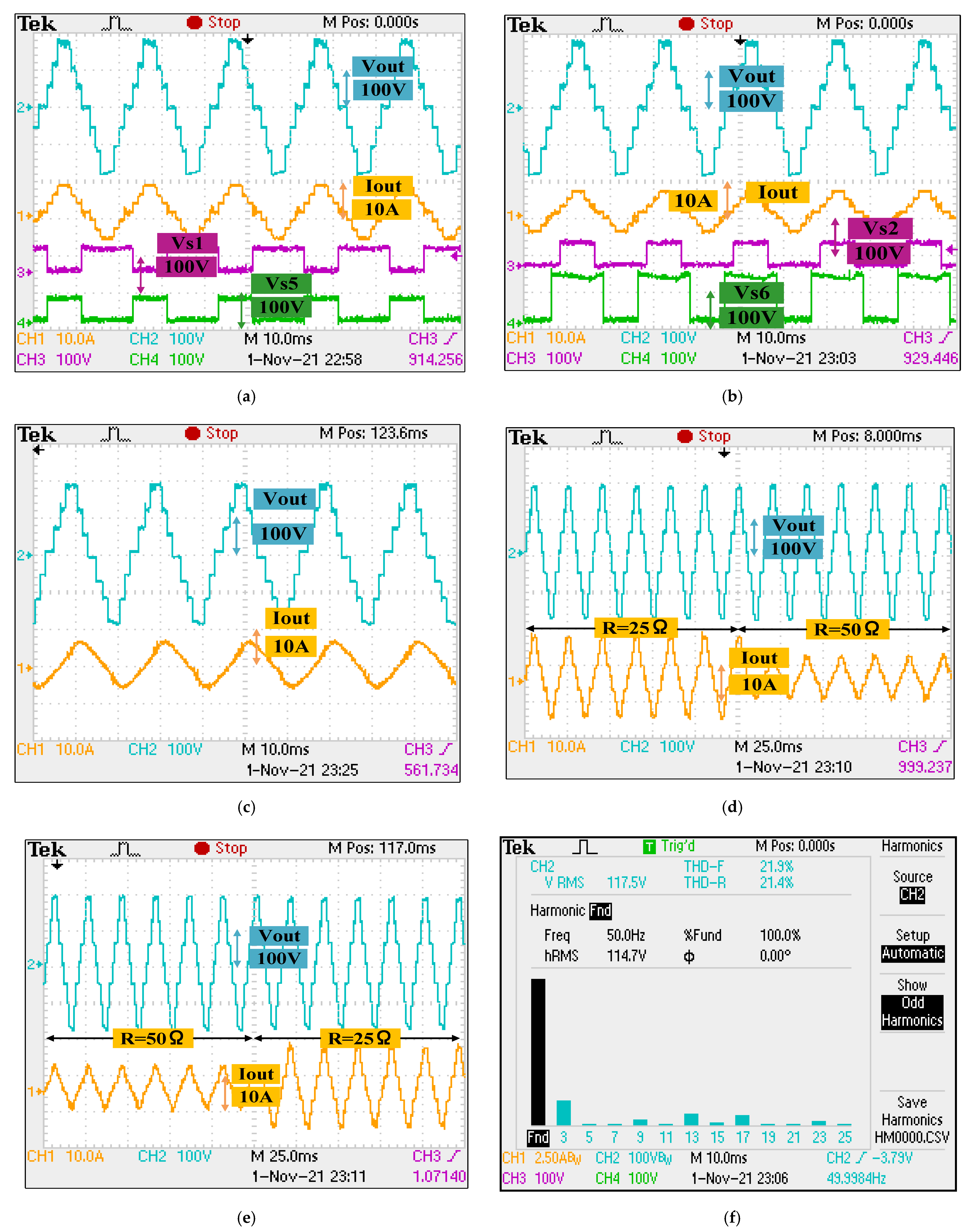Figure 8 shows the various experimental results. The output voltage, output current, and voltage stresses across switches S₁ and S₅ for a resistive load of 50 ohms are shown in Figure 8a. The peak output voltage is about 180 V, which is the sum of the input voltage sources. The output current replicates the output voltage as the load is resistive. For the same load, output waveform and voltage stresses across S₂ and S₆ are shown in Figure 8b. 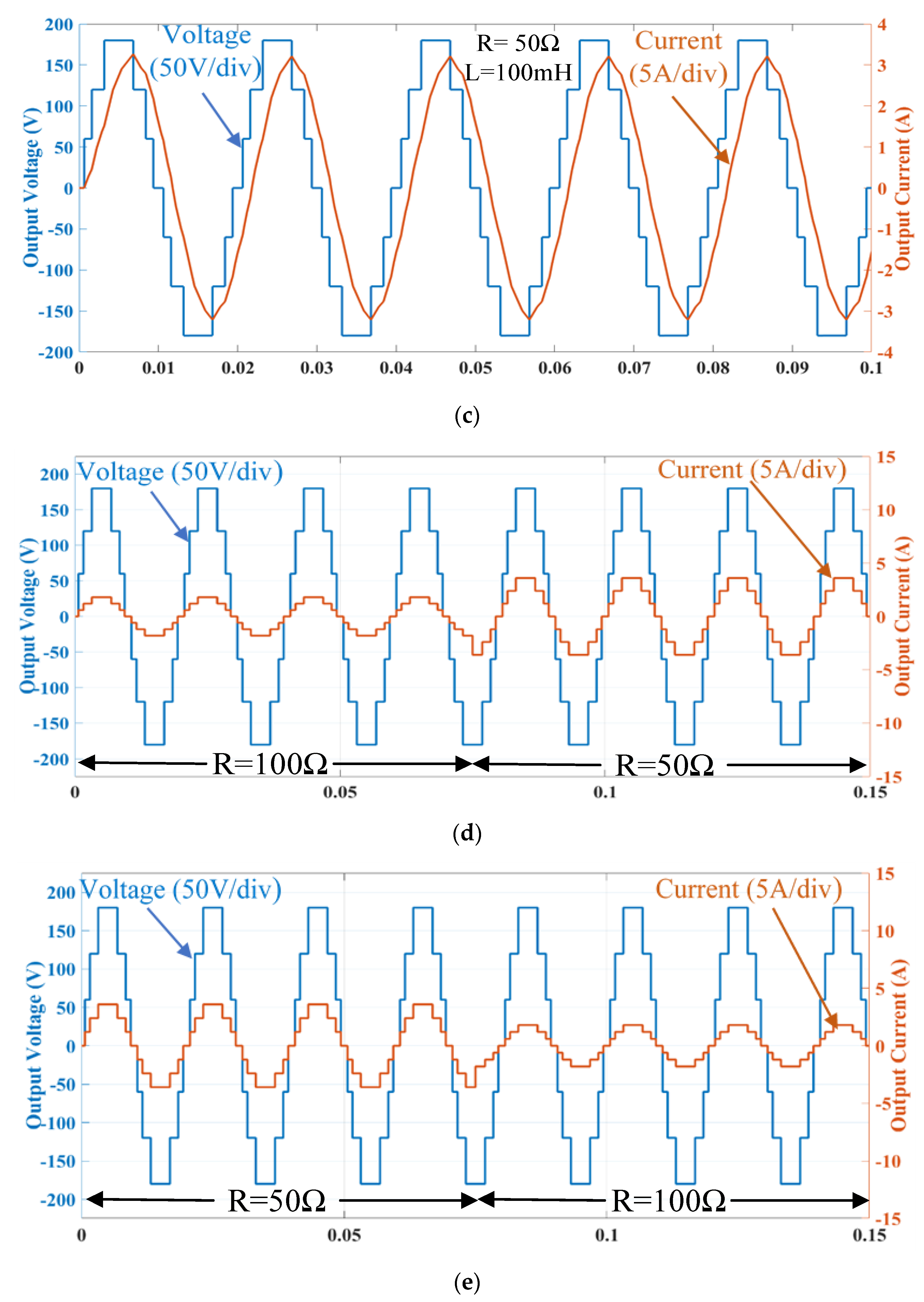Figure 8c shows the output voltage and output current for an inductive load of R = 50 ohm, L = 100 mH. The output current is sinusoidal as the load is inductive. The proposed topology has also been tested for dynamic load change, as shown in Figure 8d,e for increasing and decreasing load, respectively. The results verify that the proposed inverter is stable in dynamic loading conditions. The harmonic profile of the output voltage verifies that the fifth and seventh harmonics are eliminated, as shown in Figure 8f. The components used in this experiment have been listed in

Table 5. Experimental Parameters.

S. No.	Components/Parameters	Specifications	No. of Components
1.	Insulated-Gate Bipolar Transistor (IGBT)	FGA25N120	6
2.	IGBTs Driver circuit	TLP 250 H, ±12 V, 1 A	6
3.	DSP Board	TMS320F28335 (Texas Instruments)	1
4.	Power Supply	60 V, 120 V	2
5.	Load	50 Ω, 100 Ω, L = 100 mH	1
6.	Frequency (Fundamental)	50 Hz	_

.

6. Conclusions

A seven-level modified H-bridge inverter with a reduced component count and reduced THD is presented in this paper. Two DC sources with six IGBTs have been used to generate a seven-level output voltage, and the Aquila Optimizer (AO) has been implemented to control the output voltage with a feature to eliminate 5th and 7th harmonics. Simulation has been done in MATLAB/Simulink environment. The result shows that the AO gives a better result for a range of modulation indices than many of the well-known meta-heuristic algorithms like GA and DE. Comparison of the presented topology with other well-established topologies has also been done. Experimental results obtained verified the findings of the simulation and theoretical analysis.