Comparative Analysis of Rankine Cycle Linear Fresnel Reflector and Solar Tower Plant Technologies: Techno-Economic Analysis for Ethiopia

Abstract

The need to meet the world’s growing demand for energy in an environmentally sustainable manner has led to the exploration of various renewable energy (RE) resources for power generation. The objective of this study is to examine the techno-economic potential of concentrated solar power plants (i.e., linear Fresnel reflector (LFR) and central receiver system (CRS) for electricity generation in Eastern African countries with a case study on Ethiopia. The study was conducted using the System Advisor Model (SAM). In order to estimate the economics of the two power plants, the Levelized cost of energy (LCOE) and the net present value (NPV) metrics were used. According to results obtained from the simulations, the LFR produced annual energy of 528 TWh at a capacity factor (CF) of 60.3%. The CRS also produced a total of 540 TWh at a CF of 61.9%. The LCOE (real) for the CRS is found to be 9.44 cent/kWh against 10.35 cent/kWh for the LFR. The NPV for both technologies is found to be positive for inflation rates of 2% and below. An inflation rate above 2% renders the two power plants financially impracticable. A real discount rate above 9% also renders both projects economically unviable. Based on the obtained results, the CRS system is identified as the best technology for electricity generation under the Jijiga climatic condition in Ethiopia.

1. Introduction

Expanding access to clean and affordable energy remains one of the key policies of governments around the globe, particularly those from emerging economies [1]. Therefore, renewable energy (RE) development worldwide has seen enormous growth in recent periods due to the negative impact of fossil fuel-generated energy on the environment [2,3]. More RE capacity was added globally in 2015, surpassing fossil fuel sources for the first time. The development of RE in developing countries also surpassed that of advanced countries during that same period [4].

Notwithstanding this progress in the RE sector, many developing countries still struggle to meet the demand for electricity by their people; this is even more acute in Sub-Saharan Africa [4,5]. Energy generation from renewable resources is seen as Africa’s future in relation to electricity generation due to its robust and sustainable nature [6]. The African continent is in an exclusive position to benefit from the socio-economic and environmental benefits in relation to the development and use of renewable resources to meet the continent’s increasing demand for energy more sustainably due to its enormous RE resources [7].

Concentrating solar power (CSP) is a type of RE that relies on concentrated solar irradiation to generate high-temperature heat, which is then used in a power block to produce electrical energy [8]. CSP technologies capture the sun’s heat using mirrors to heat, either solids, liquids, or gases, to a temperature between 400 °C and 1000 °C, which produces steam to turn heat turbines to generate electricity [9]. The CSP technology appears not to be a good option for generating distributed energy but rather large-scale systems, unlike the photovoltaic technology. CSP technology can be combined with thermal energy storage (TES) or another power technology (i.e., hybrid system), providing power at a fixed capacity and customized. CSP technologies are appropriate for regions exposed to more solar radiation, particularly the direct normal irradiation (DNI); such areas are North Africa, Southern Europe, South Africa, Middle East, China, sections of India, Australia, and Southern United States [10]. There are presently four types of CSP technologies; these are linear Fresnel reflector system (LFR), parabolic dish or engine system (DE), parabolic trough collector system (PTC), and solar tower, also called central receiver system (CRS). The type of solar tracking, mirrors, and the energy-saving mechanisms of these technologies vary. However, they all function under the same principle, i.e., a steam turbine (heat engine) stimulation to generate electrical power. The PTC is the most commercially advanced system compared to the other forms [10,11].

Renowned researchers have done several studies to ascertain the techno-economic potentials of CSP technologies at various sites worldwide. Rashid et al. [12] analyzed the techno-economic of a CSP plant, which was hybridized with TES and natural gas systems. Their results show that incorporating a TES controls power production by the natural gas and solar energy systems during the day. It also led to the increase in the solar fraction of the hybrid system, while it caused a relatively small reduction in the thermodynamic efficiency. The hybrid plant with thermal energy storage (TES) system had a Levelized cost of energy (LCOE) of 86.32 $/MWh against 74.92 $/MWh for the single natural gas plant. Islam et al. [13] conducted a techno-economic valuation on the potential of CSP technologies for Malaysia’s RE sector. They analyzed three different types of CSP, i.e., PTC, CRS (solar tower), and DE, under varying economic conditions. Their results show that the PTC and the CRS systems are most suitable for East and Peninsular Malaysia sites. However, the PTC system was the best with regard to the simple payback period, net present value (NPV), and internal rate of return (IRR). Aly et al. [14] also investigated the techno-economic of two different CSP technologies (PTC and ST) in Tanzania. The obtained LCOE under debt interest rate according to their study for the ST power plants ranges from 11.6 ¢/kWh to 12.5 ¢/kWh, while that of the PTC ranged from 13.0 ¢/kWh to 14.4 ¢/kWh. Furthermore, Abaza et al. [15] executed a techno-economic investigation on a 10 MW CSP. The study proposed three simple power blocks, namely: Steam Rankine Cycle (SC), Open Gas Cycle (GC), and Organic Rankine Cycle (OC), with the help of the ASPENHYSYS software to optimize the performance parameters. The LCOE obtained for the SC as a power block was 0.0947 $/kWh which is less than the OC and GC by 48.8% and 31.82%, respectively. Agyekum and Velkin [16] also evaluated the technical and economic potential of two different CSP technologies (PTC and ST) for the Ghanaian RE sector. In their study, the ST installed in Tamale recorded an LCOE of 13.67 cent/kWh against 14.73 cent/kWh for that of Navrongo, while the PTC at Navrongo and Tamale had 25.83 cent/kWh and 28.83 cent/kWh. Zayed et al. [17] also experimentally established and thermodynamically modeled a 25 kW Solar Dish/Stirling under the weather conditions of Tianjin in China. Their results indicate that the Solar Dish/Stirling system generated 28.748 MWh of electricity yearly at a net general efficiency of 19.55% and an LCOE of 0.2565 $/kWh. Boukelia et al. [18] also analyzed two PTC power plants integrated with TES and a fuel backup system in Algeria. According to their obtained results, molten salt appears the best technology because of its low investment cost below $360 million and lower LCOE of 8.48 cent/kWh. Tamanrasset was identified as the best site for constructing a parabolic trough solar thermal power plant because the lowest LCOE of 7.55 cent/kWh was recorded at that location. Trabelsi et al. [19] evaluated the performance of PTC power plant in southern Tataouine in Tunisia. Results from their simulation suggest an excellent outcome relative to the dry cooled CSP power plant, an LCOE of 18.28 cent €/kWh was obtained. Belgasim et al. [20] worked on the potentials of CSP technologies, i.e., PTC, for the Libyan electricity sector. An LCOE of 24 $/kWh was obtained for the CSP plant with a total installation cost projected per net capacity of 8.3 thousand dollars per kilowatt at an absolute cost of about 412 million US dollars. Agyekum et al. [21] estimated the effect of different heat transfer fluids i.e., Salt (46.5% LiF 11.5% NaF 42% KF) and Salt (60% NaNO₃ 40% KNO₃) on a CRS in China. Their results indicated that the system with salt (60% NaNO₃ 40% KNO₃) recorded a real LCOE of 0.1668 $/kWh using a Rankine cycle, while the system with salt (46.5% LiF 11.5% NaF 42% KF) recorded the lowest real LCOE of 0.1586 $/kWh using supercritical carbon dioxide (sCO₂) cycle.

Research has shown that there exists a bi-directional nexus between poverty and access to energy, i.e., the non-availability of clean, cheap, and modern forms of energy leads to an increase in the levels of poverty of an individual or country and retards the development of modern energy sources [22]. Ethiopia is the second-most populous country in Sub-Saharan Africa. Most of the people who live in this country, particularly those in far-flung areas, face the lack of clean and reliable energy supply, leading to the dependence on traditional sources of energy generation for cooking, lighting, and heating. More than 90% of the population of Ethiopia rely on biomass for cooking which has led to the cutting down of trees leading to a drastic reduction in the country’s natural forest cover [23]. The World Health Organization (WHO) has estimated that about 72,400 deaths per annum are recorded in Ethiopia due to indoor air pollution [22]. Ethiopia is among the countries that receive high solar irradiation; the DNI at certain parts of the country is within the acceptable range for CSP power plant development, as shown in Figure 1, which Solargis develop for the World Bank Group [24]. Despite this enormous resource, the country is yet to develop it to benefit the people. Although the country receives the needed DNI capable of supporting CSP development, there is little information on their bankability relative to investments.

In this study, two different CSP technologies, i.e., CRS and LFR, are studied to assess their techno-economic potentials at Jijiga in Ethiopia to fill the research gap. This study is important because these power plants have seen many advancements in technologies, resulting in reduced costs in recent times. Therefore, it is essential to conduct a full study on the performance of such systems for possible integration into the country’s electricity generation setup. Unlike most existing literature which cover just the economics and energy output of such systems, this study goes beyond that to identify critical technical parameters and the optimal financial conditions suitable for the design of the two systems. These parameters are key to the design and development of the two CSP technologies for Ethiopia and other countries in that enclave with similar CSP potentials. This study is the first of such studies for the country, allowing policymakers and investors to compare the techno-economic of two potential power generating systems in just one study. The paper consists of 5 sections; the geographical location and principles of CSP technologies are presented in Section 2, the methodology and materials adopted for the assessment are provided in Section 3, the results and discussion are provided in Section 4, and the conclusion is presented in Section 5.

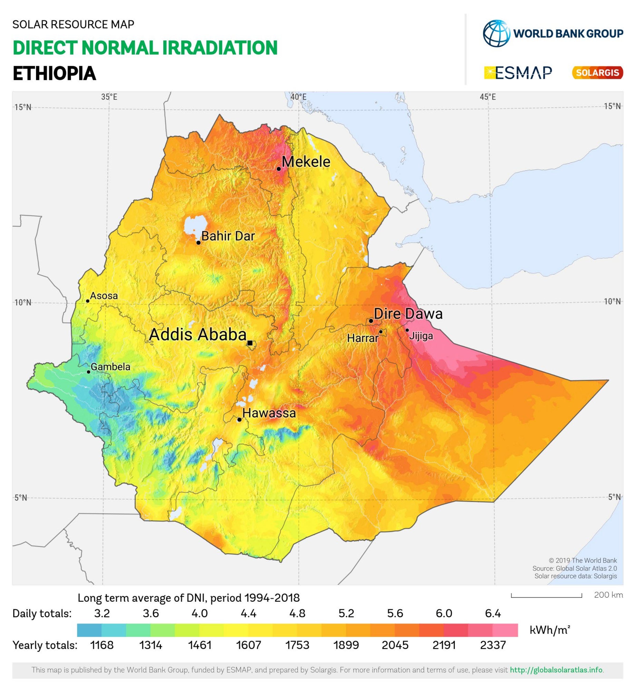
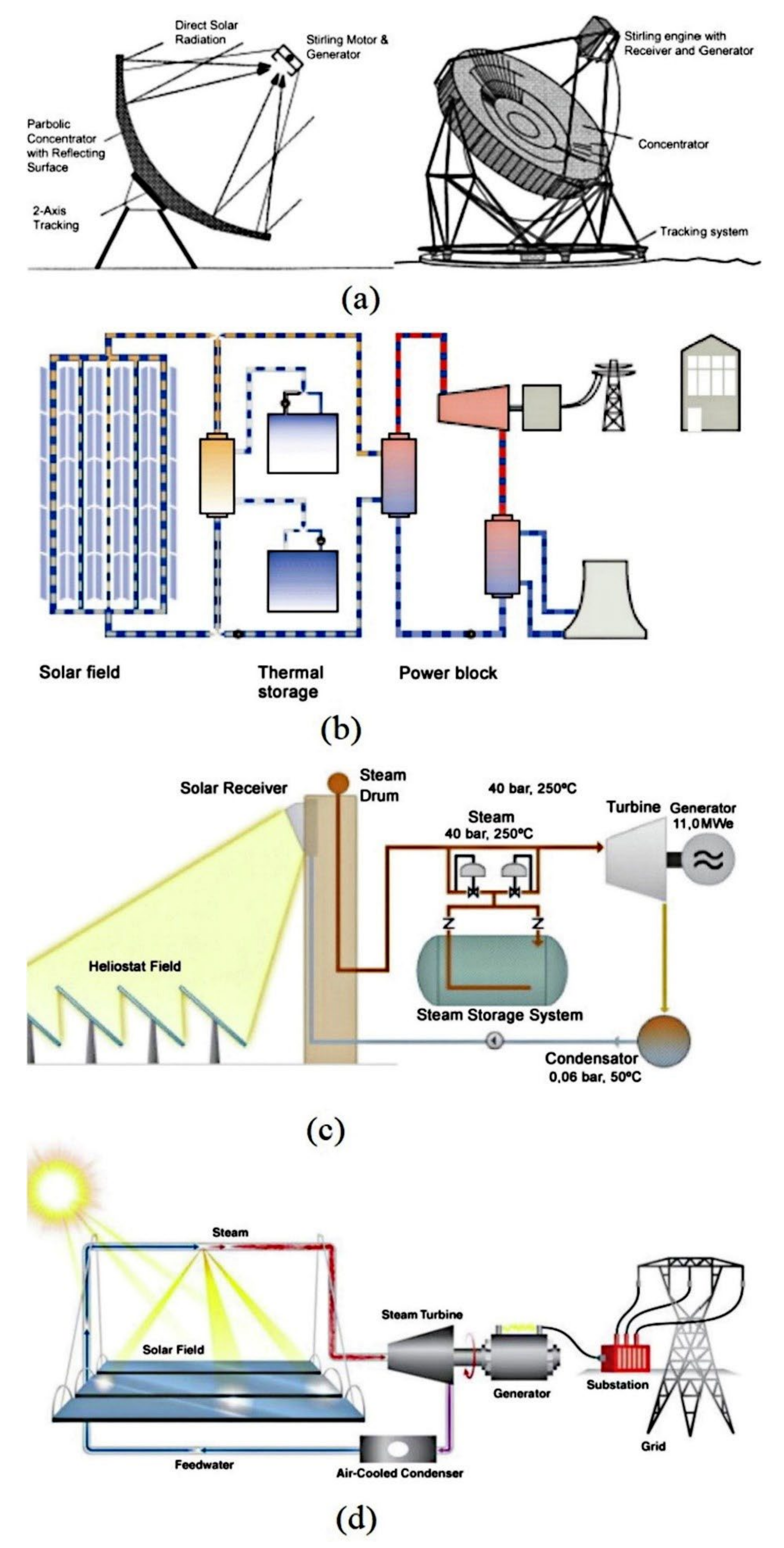
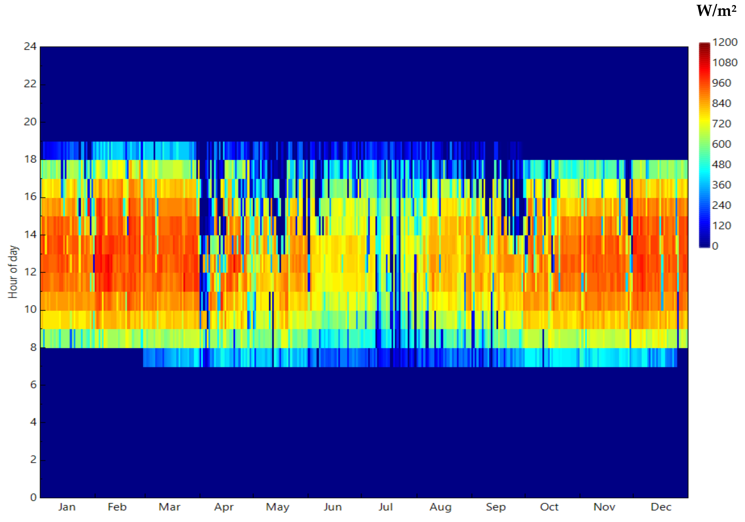
2. Geographical Location Requirements and Principles of CSP Technologies

CSP technologies mostly thrive well in regions or countries with high DNI, such as those in high altitudes with very little scattering and absorption of sunlight. Research shows that the CSP technology performs well with a minimum DNI range of 1900–2000 kWh/m²/year [16]. Figure 2 shows the types of CSP technologies.

The LFR is a modified form of the PTC, instead of using big troughs for the concentration of the solar flux, the trough is divided into long rows of slightly curved or flat mirrors, which is approximately the parabolic shape of a trough, it concentrates the flux which is comparable to that of a trough. A downward-facing linear fixed trough absorbs the concentrated flux. High operating temperature, direct steam generation, and multistage heating are the main characteristics that support its wide spectrum deployment [25]. LFRs do not have a parabola arrangement for the rows; rather, the primary optics are flat. Another very important point is that LFRs have a fixed receiver, unlike PTCs.

The CRS is made of hundreds to thousands of small reflectors fixed on the ground. These reflectors concentrate the radiations from the sun onto a central receiver fixed on top of a tower. Due to the very high temperatures, molten salts or direct steam generation are normally used as a heat-absorbing medium [16,25].

The beam from the sun’s radiations concentrates on the focus of the parabolic trough. A linear absorber is placed at the focal line to absorb the energy [25].

3. Methodology and Materials

The System Advisor Model (SAM) is employed in this study to simulate two different CSP technologies, i.e., CRS and LFR. The United States Department of Energy’s National Renewable Energy Laboratory developed the SAM software. SAM is a techno-economic software that evaluates a RE power project’s technical output and financial characteristics. It is used by policymakers, project developers, researchers, and equipment manufacturers in assessing the financial, incentives options, and technologies for RE projects. The financial models in the SAM computer software are for power plants that either sell or buy electricity at retail rates (commercial and residential) or sell electricity at a fee determined in a power purchase agreement (PPA). The tool facilitates sensitivity and parametric analyses, studies of weather variability (P50/P90), and Monte Carlo simulation [26]. Several studies on CSP techno-economics have been conducted using this tool, such as that presented in [14,16,27,28].

3.1. Technical Analysis

Accurate hourly DNI estimation for a particular location is needed for CSP simulation. This study used data from the European Commission’s Photovoltaic Geographical Information System (PVGIS) [29] for the simulation to get an accurate DNI for the studied location. The data was downloaded in the Typical Metrological Year (TMY) format. The location for the simulation is geographically located on latitude 9.4° N and longitude 42.8° E at an elevation of 1706 m. Jijiga was selected for this feasibility study because the DNI of this area is very high. The average temperature and wind speed for Jijiga are 19.4 °C and 3.7 m/s, respectively, according to data from the Photovoltaic Geographical Information System (PVGIS). Scattering of solar radiation between the surface and atmosphere of the earth plays a major role when calculating the geometrical and spectral distribution of sky radiance paths [30,31]. The irradiance from solar is non-stationary, so this process depends on the day and time of the year. The monthly DNI figures for the study area are illustrated in Figure 3. The solar radiation can be estimated using the zenith angle $\left({\theta }_z\right)$ which is deterministic; hence, the earth’s position around the sun can be computed using Equation (1) [30].

$$cos{\theta }_z=sin\phi sin\delta +cos\phi cos\delta cos\omega$$

(1)

where $\delta$ represents the declination angle, $\omega$ denotes the hour angle, which is zero at solar noon, negative and positive in the afternoon and morning(s), respectively, and $\phi$ is the latitude.

The declination and sunset hour angle can be calculated using the following equations. Equations (2)–(7) were obtained from Ref [30].

$$\delta =23.45 sin\left\{\left(\frac{360}{365}\right)\left(284+n\right)\right\}$$

(2)

where $n$ is the day of the year which starts from the first of January.

$$\omega =co{s}^{-1}\left(-tan\phi tan\delta \right)$$

(3)

The monthly average global radiation $H$ and the sunshine hours $S$ daily based on the regression of first order.

$$\frac{H}{H_o}=a+b\frac{S}{S_o}$$

(4)

where, $S_o$ represents the maximum number of sunshine hours or length of the day which is computed using Equation (5). $H_o$ denotes monthly average day-to-day extraterrestrial radiation, $a$ and $b$ represent empirical coefficients.

$$S_o=\frac{2}{15}co{s}^{-1}\left(-tan\phi ·tan\delta \right)$$

(5)

In the case of CSP, the DNI directly impacts electricity generation, which can be calculated using Equation (6).

$$I=K_c I_{cs}$$

(6)

where, $K_c$ and $I_{cs}$ represent the clearness index and clear sky DNI, respectively. The clear sky DNI is usually calculated using the Beer-Lambert law in the radiative transfer model.

$$I_{cs}=I_o e^{-m\tau }$$

(7)

where $\tau$ and $m$ are the depth of the atmosphere and the relative air mass, respectively. $I_o$ denote the total solar irradiance.

The rainy season in Ethiopia generally starts in April and ends in September; however, each part of the country has its own rainfall pattern. The rainy period for the selected site starts in March to April for the short season, while the long rainy season commences from July to September. The driest months are November and February [32]. This accounts for the drop in DNI in the rainy months due to the formation of clouds and the relatively high DNI for the dry months due to clear skies. The area records a DNI (beam) of 7.18 kWh/m²/day, diffuse horizontal of 1.79 kWh/m²/day, and a global horizontal of 6.82 kWh/ m²/day.

The technical data used for the simulation of the various power plants in this study are presented in

Table 1. Technical specifications for the simulation.

Linear Fresnel Reflector (LFR)			Solar Tower
Description	Features	Value	Description	Features	Value
Solar field	Solar multiple	3	System design	Solar multiple	3
	Field aperture	850,000 m2		HTF hot temperature	574 °C
	Number of collector modules in a loop	16		HTF cold temperature	290 °C
	Number of subfield headers	2		Full load hours of storage	12 h
	HTF pump efficiency	0.85		Design turbine gross output	111 MWe
	Stow angle	170° [34]		Estimated net output at design (nameplate)	100 MWe
	Field HTF	Hitec Solar Salt		Cycle thermal power	269 MWt
	Field HTF min operating temp.	238 °C	Heliostat field	Heliostat width	12.2 m [35]
	Field HTF max operating temp.	593 °C		Heliostat height	12.2 m [35]
	Design loop inlet temp.	293 °C		The ratio of the reflective area to profile	0.97
	Target loop outlet temp.	391 °C		Single heliostat area	144.375 m2
	Single loop aperture	7524.8 m2		Total land area	1892 acres
	Loop optical efficiency	0.61		Base land area	1847.04 acres
	Solar field area	405.35 acres	Tower and Receiver	Receiver thermal power	808.3 MWt
	Total land area	648.57 acres		Coating emittance	0.88
	Loop thermal efficiency	0.98		Receiver height	21.60 m [36]
Collector and Receiver	Reflective aperture area of the collector	470.3 m2		Receiver diameter	17.65 m
	The length of the collector module	44.8 m		Number of panels	20
	Length of crossover piping in a loop	15 m		HTF type	Salt (60% NaNO3 40% KNO3)
	Absorber tube inner diameter	0.066 m	Power cycle	Power block startup time	0.5 h
	Absorber tube outer diameter	0.07 m	Rankine cycle	Boiler operating pressure	100 Bar
Power cycle	Reference output electric power at design condition	111 MWe		Steam cycle blowdown fraction	0.02
	Estimated net output at design (nameplate)	100 MWe		Condenser type	Evaporative
	Rated cycle conversion efficiency	0.36	Thermal storage	Storage type	Two tanks
	Cycle design HTF mass flow rate	2118.5 kg/s		TES thermal capacity	3233 MWt-hr
Rankine cycle	Boiling operating pressure	100 Bar		Available HTF volume	7453 m3
	Condenser type	Evaporative		Initial hot HTF percentage	30%
Thermal storage	TES hours	12 h		Tank height	12 m
	Total tank volume	18,819 m3		Tank diameter	41.7 m
	TES thermal capacity	3358.52 MWht		Storage tank volume	16,408 m3
	Min Fluid volume	940 m3		Cold tank heater capacity	15 MWe
	Tank diameter	34.61 m		HTF density	1808.48 kg/m3

. These parameters were adopted from the SAM software, except a citation is provided. A 0.2% degradation rate per annum was used for both systems, which is acceptable in CSP technologies [16,33].

Solar multiple (SM) can be described as the area of the field aperture expressed as a multiple of the area of the aperture needed to run the power cycle at its design capacity. It can be mathematically calculated using Equation (8) [37].

$$SM=\frac{Power cycle capacity}{Solar field capacity}$$

(8)

The output for a solar field design (SFD) is the delivered thermal energy by the solar field under design conditions for a particular SM. The output of SFD can be computed at the interface of the power block and receiver as a function of the SM mathematically using Equation (9) [37].

$$Q_{sf,des}=\frac{W_{pb.des}}{{\eta }_{des}} SM$$

(9)

where, $Q_{sf,des}$ represents the SFD heat output, $W_{pb.des}$ is the design work out from the power block, ${\eta }_{des}$ denotes the design efficiency.

3.2. Economic Analysis

This section describes the mathematical models used to calculate each system’s economics and life cycle analysis. The technical inputs and assumptions for the study are also provided in this section. To evaluate the economics of the two power plants, the LCOE and the NPV metrics were used.

The LCOE is the ratio of the complete cost accrued in the lifetime of the project to the unit of electricity produced during that same period [16,38]. The SAM program computes both the nominal LCOE and real LCOE for the project. The real LCOE is the constant dollar value, whereas the nominal LCOE is defined as the current dollar value. The real LCOE was used in the analysis in this study since it accounts for the inflation that may occur over the project’s lifetime, making it the optimum metric for long-term analysis of such projects [16]. The LCOE can be computed using Equations (10) and (11) [14,16,39].

$$LCO{E}_{\left(r\right)}=\frac{-C_o-\frac{{{\displaystyle \sum }}_{n=1}^N{C}_n}{{\left(1-d_n\right)}^n}}{\frac{{{\displaystyle \sum }}_{n=1}^N{Q}_n}{{\left(1-d_r\right)}^n}}$$

(10)

$$LCO{E}_{\left(n\right)}=\frac{-C_o-\frac{{{\displaystyle \sum }}_{n=1}^N{C}_n}{{\left(1-d_n\right)}^n}}{\frac{{{\displaystyle \sum }}_{n=1}^N{Q}_n}{{\left(1-d_n\right)}^n}}$$

(11)

where $LCO{E}_{\left(r\right)}$ represent the real LCOE, $LCO{E}_{\left(n\right)}$ is the nominal LCOE, $Q_n$ is the electricity produced by the power plants in $N$ years, $C_o$ denote the equity investment of the project, $N$ represents the analysis period, $C_n$ is the annual cost of the project in number of years, $d_n$ is the nominal discount rate, $d_r$ is the real discount rate.

Another indicator used in comparing the economics of power plant projects is the NPV. The NPV and the LCOE are used to compare different power plants with varying installed capacities, capacity factors, and investment structures. The NPV is calculated by shifting back all the costs and revenues to the beginning of the project by means of a discount rate. The NPV considers both revenues and costs; this is estimated using Equation (12) [14,36]. A positive NPV shows that the intended project is financially viable, whereas a negative value indicates otherwise [14,16,21].

$$NPV={\displaystyle \sum }_{n=0}^N\frac{C}{{\left(1+D\right)}^n}$$

(12)

where $C$ is the after-tax returns of the project, $N$ is the analysis period in years, and $D$ denotes the nominal discount rate.

The LCOE has no restrictions in terms of the scale of the project; it is therefore considered a superior metric for the economic assessment of projects with considerable differences in their scale. This is because large-scale projects generally come with a corresponding large NPV compared to small-scale projects; hence the NPV is not an appropriate metric for assessing the pros and cons of such projects [16,40]. The specific financial parameters adopted for this study are presented in

Table 2. Specific parameters used in the simulation.

Description	Value	Reference
Analysis period	25 years	[16]
Income tax rate	30% per annum	[41]
Insurance rate (annual)	0.5% of installed cost	[33]
Real discount rate	10% per annum	[16]
Nominal discount rate	12.75%
Inflation rate	2.5%	[36,42]
Tenor	18 years	[16]
Sales tax	15% of total direct cost	[41]
Annual interest rate	10%	[33]

.

The economic parameters used in simulating the various CSP technologies are also presented in

Table 3. Input financial parameters for the various systems [44].

Category	Description	LFR	CRS
Direct capital costs	Site improvements	20 $/m2	16 $/m2
	Solar/Heliostat field	150 $/m2	140 $/m2
	HTF system	47 $/m2
	Storage	32 $/kWht	22 $/kWht
	Power plant	1100 $/kWe
	Tower cost fixed	-	3,000,000 $
	Receiver reference cost	-	103,000,000 $
Indirect capital costs	EPC and owner cost	11%	13%
	Sales tax of direct cost	80%	80%
	Land cost per acre	800 $	800 $
Operation and Maintenance costs	Fixed cost by capacity	66/kW-yr	66/kW-yr
	Variable cost by generation	4 $/MWh	3.5 $/MWh

. The input parameters with respect to the cost of the various categories of the two different CSP systems in this study can be classified into three, i.e., direct capital cost, indirect capital cost, and operations and maintenance costs. The SAM program has default cost inputs for the various CSP options, reflecting the best estimates of the systems in the perspective of the National Renewable Energy Laboratory (NREL) in the United States at the time of the release of the SAM version [14,43]. This study used the current version, SAM 2020.2.29 released recently for the analysis; for that reason, the input parameters used in the simulation are therefore acceptable.

Normally, a power purchase agreement (PPA) is a contract that exists between a private utility company and a government. The private entity or company produces electricity through an agreement for an agency of government over an agreed period of time. Such agreements usually last between 15 and 25 years [45]. The PPA model is the best financial model for large-scale power projects such as the one modeled in this study. Commercial PPA and utility projects are presumed to sell the generated electricity through a PPA at a fixed price with optional yearly escalation and time-of-delivery factors [21,46]. This study used the PPA Single Owner financing structure for the simulation and analysis.

4. Results and Discussion

This section covers the results and discussion. It is divided into economic, technical, and sensitivity analysis parts.

4.1. Economic Analysis

The CRS recorded the least real LCOE. However, both two systems will not be economically viable under the current financial assumptions for the study; this is because of the negative NPV recorded by both technologies. A summary of the simulated results for the base case parameters for the two technologies are presented in

Table 4. Results from the simulation using the assumed financial parameters for the study.

Metric	LFR	CRS
PPA price (year 1), ¢/kWh	10.54	9.78
Levelized PPA price (nominal), ¢/kWh	12.57	11.47
Levelized PPA price (real), ¢/kWh	10.34	9.44
LCOE (nominal), ¢/kWh	12.58	11.48
LCOE (real), ¢/kWh	10.35	9.44
NPV, $	−170,654	−289,498
Internal rate of return (IRR), %	11	11
Year IRR is achieved, years	20	20
IRR at end of project, %	12.73	12.72
Net capital cost, $	853,748,096	793,734,464
Equity, $	357,093,248	332,979,712
Size of debt, $	496,654,880	450,754,752

.

In September 2019, the cost of electricity in Ethiopia was 0.010 $/kWh and 0.018 $/kWh for households and businesses, respectively. It includes all aspects of the electricity bill to the consumer, such as taxes, cost of power, and distribution. For the purposes of comparison, the global average price of electricity during that same period was 0.14 $/kWh for households and 0.12 $/kWh for businesses [47]. It, therefore, means that electricity generation from both CSP technologies will be much expensive in the Ethiopian electricity market for consumers, but both technologies will be relatively cheaper in the global context. Moreover, comparing the obtained results to the International Renewable Energy Agency’s (IRENA) 2020 report on CSP’s, the results from both technologies in this study will be relatively less than the global weighted average, which is 0.185 $/kWh for both systems in 2018 [16,48]. Weighted average price for CSP technologies is however expected to be about 0.076 $/kWh by 2021 [48].

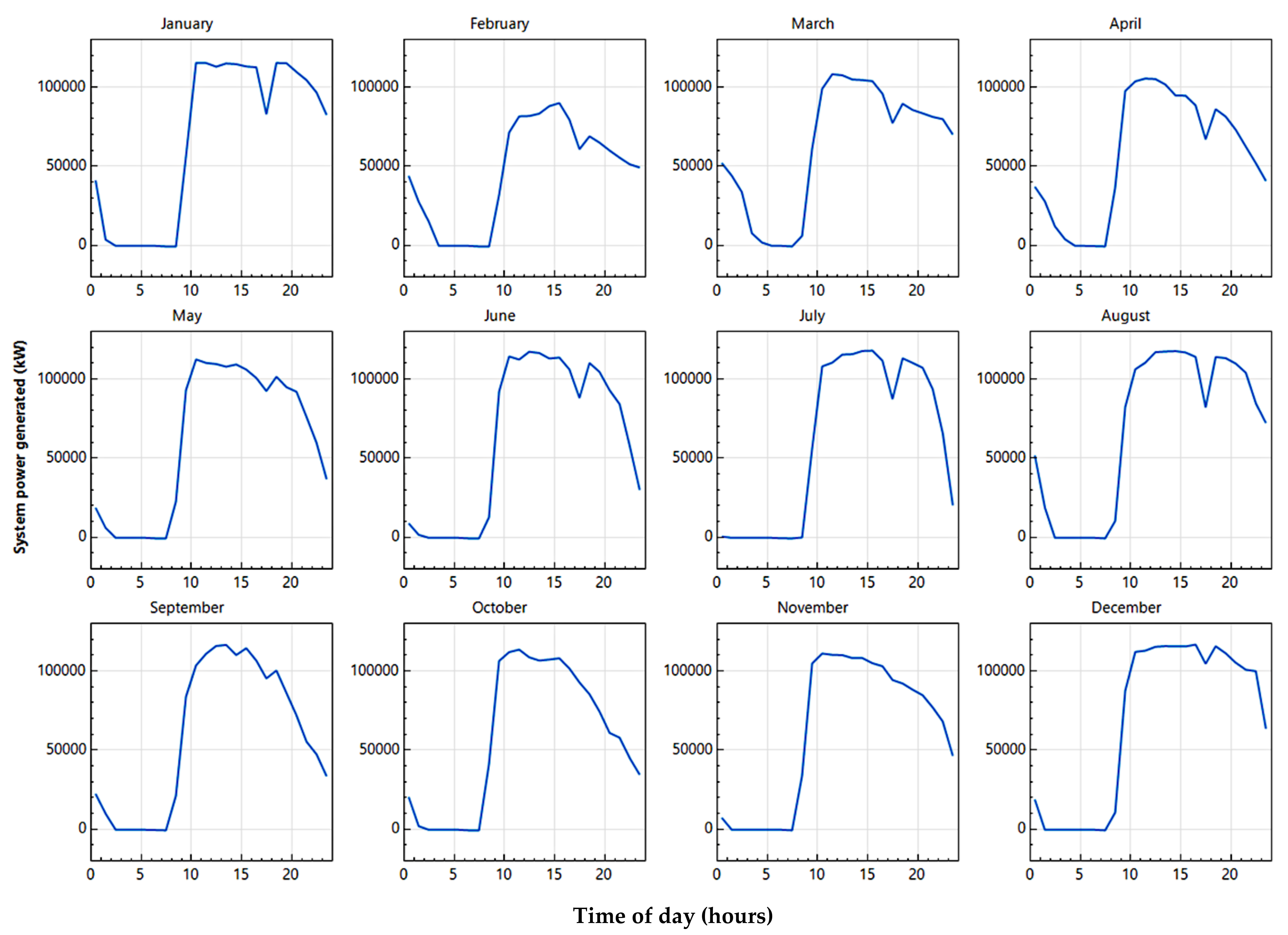
4.2. Technical Analysis for Both Systems

The LFR recorded annual energy (year 1) of 528 TWh at a capacity factor (CF) of 60.3%. The CRS also produced a total of 540 TWh energy in year one at a CF of 61.9%. The highest energy is generated in the dry seasons. CF is the ratio of the generated output electricity in a year to the maximum output generated from the power plant for a given period [21]. The CF of CSP technologies has been increasing over the years due to advancements in technologies and larger TES capacities. The obtained CF for both technologies are slightly less than the 64% published by the IRENA report for CSPs with TES above 10 h [48]. The highest cycle electrical power output for the two systems occurred in the months of December and January when DNI was high. Figure 4 and Figure 5 represent the monthly system power generated by the two power plants.

The SM is a key factor during the design stages of CSP systems; it helps determine the solar field area as a multiple of the power block’s capacity. An increase in SM normally lead to an increase in the system’s output, but overly increasing it can lead to high investment and maintenance costs [16,39]. Therefore, it is imperative to identify the optimum SM for such power plants to inform decision-making during design stages. It is observed from the analysis that the LCOE for both power plants reduces with increasing SM, which can be attributed to the increase in the produced energy due to the high quantity of flux reflected on the receiver, but it can only be up to a certain SM. Figure 6 shows the optimization analysis for the LFR system under varying TES periods. The results from the analysis indicate that the optimum solar multiple depends on the TES period as expected. The SM for all TES scenarios in this study for the LFR is dependent on the TES period.

The optimum SM for the different TES periods of the CRS are represented in Figure 7. The results show that the optimum SM for a 12-h storage period should be 2, where the least LCOE of 9.13 ¢/kWh is recorded. The optimal SM for the entire system generally ranges between 1.5 and 2.0. In the case of the CRS, increasing the TES period beyond 8 h has a comparatively inconsequential effect on the LCOE; it suggests that the TES for such a power plant can be left at 8 h. This information is critical during the design stages, and it is expected to help in any future project in that regard.

4.3. Sensitivity Analysis

It is evident that several technical and economic factors can either positively or negatively affect the viability of power plant projects. Therefore, it is very important to assess the effect of certain parameters on the techno-economic performance of both systems to ascertain their impact on the bankability of the projects. In the case of economics, some financial parameters such as discount rate and inflation rate were varied to assess their impact on the LCOE and the NPV of both projects. Some technical parameters were also varied to evaluate their effect on the economic and technical performance of the power plants.

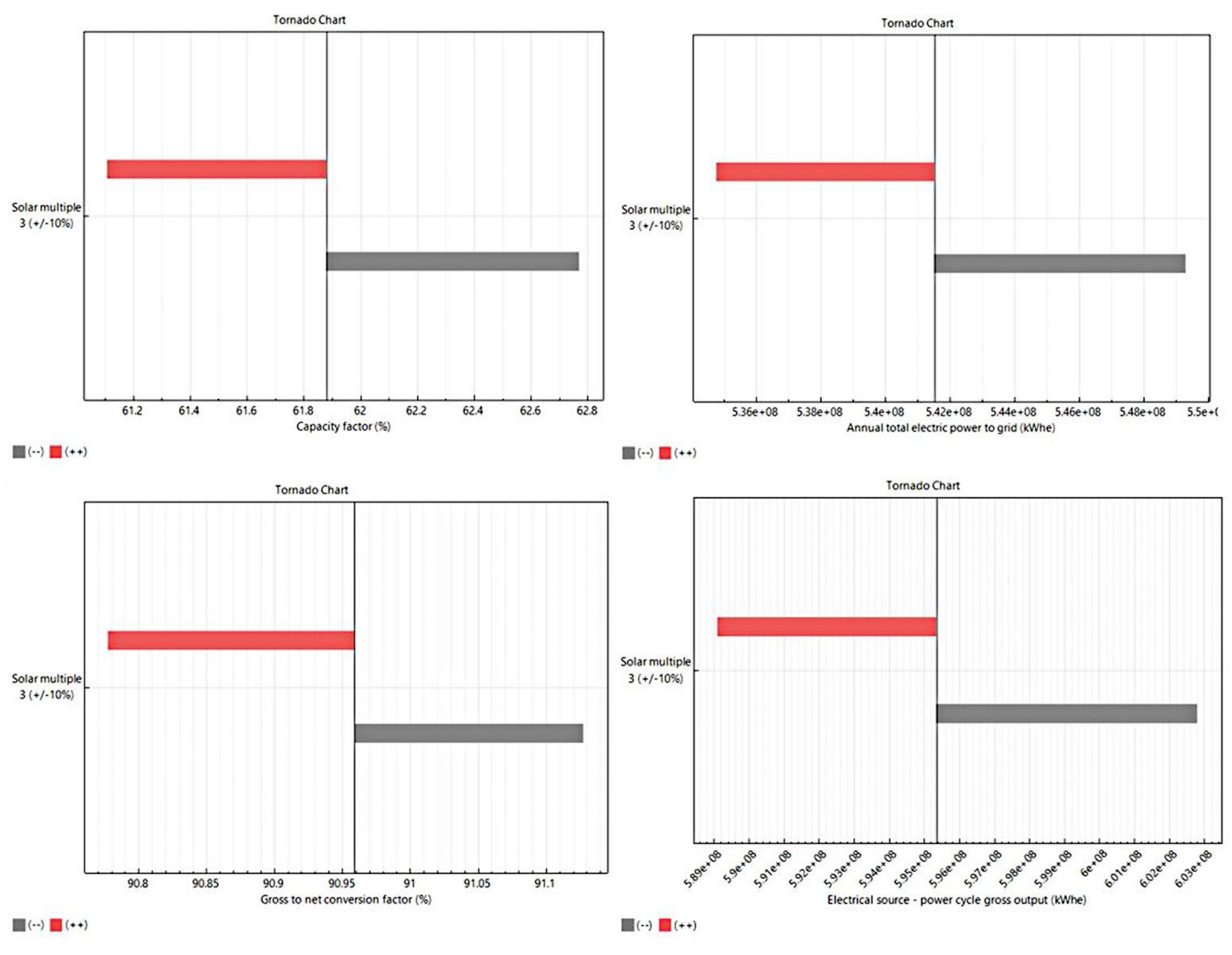
4.3.1. Technical Sensitivity Analysis

A sensitivity analysis was conducted using the macros tool in the SAM program to estimate the effect of certain parameters on the technical performance of the simulated power plants using an uncertainty of ±10%. A negative correlation signifies that a lower parameter value results in a higher value for the LCOE, while a positive correlation denotes a higher value for the input parameter results in higher LCOE values. The annual energy production, capacity factor, electricity source—power cycle gross output, and gross to net conversion factors were evaluated and presented in Figure 8 and Figure 9. As can be seen from the two figures, increasing/decreasing an SM increases/decreases the capacity factor, annual energy production, gross to net conversion factor, and the electricity source—power cycle gross output for both power plants. This can be attributed to the fact that a lower/higher solar field area leads to either a lower or higher SM, which significantly affects energy production. Hence, uncertainties in SM will have a corresponding impact on the performance of both systems.

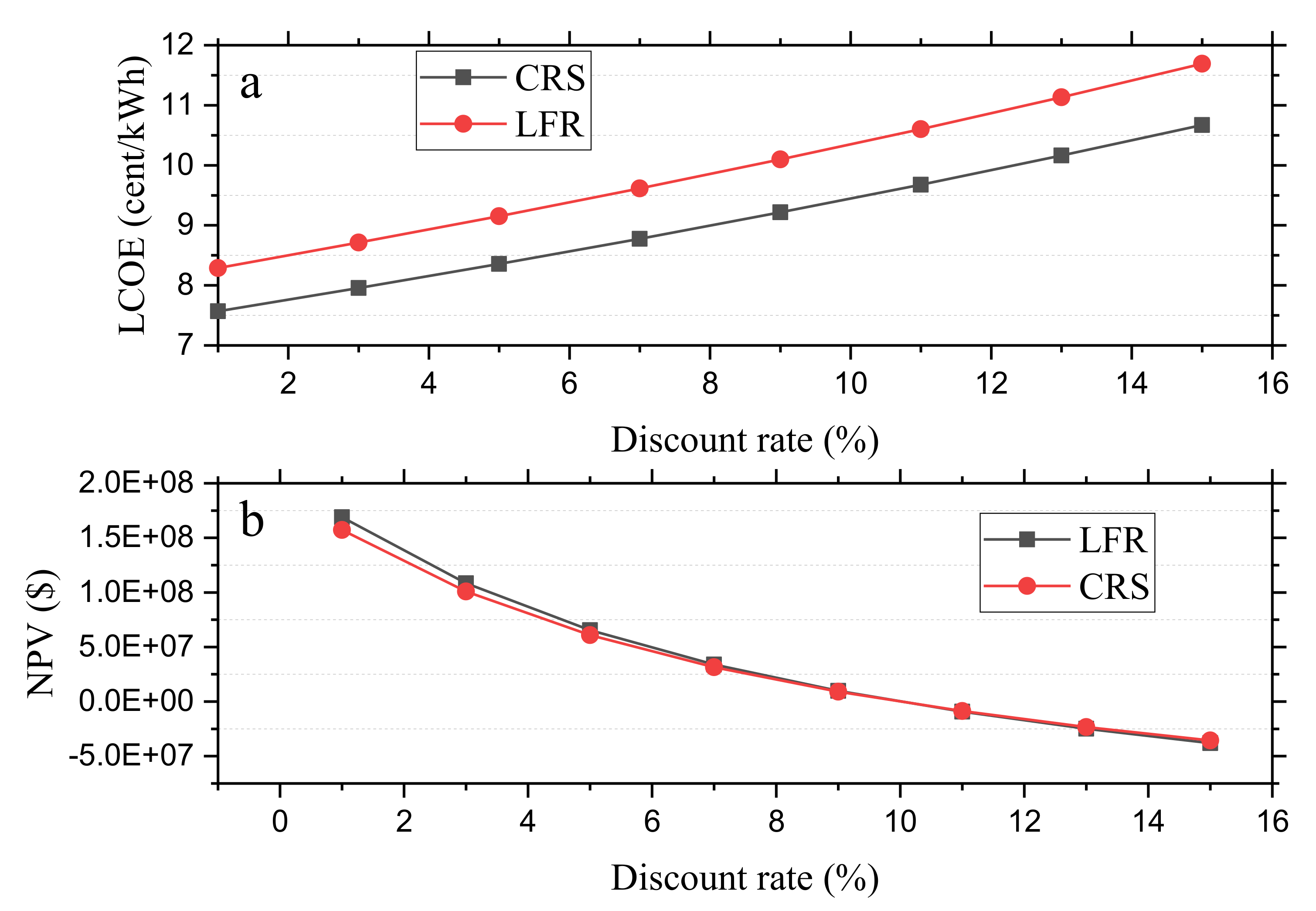
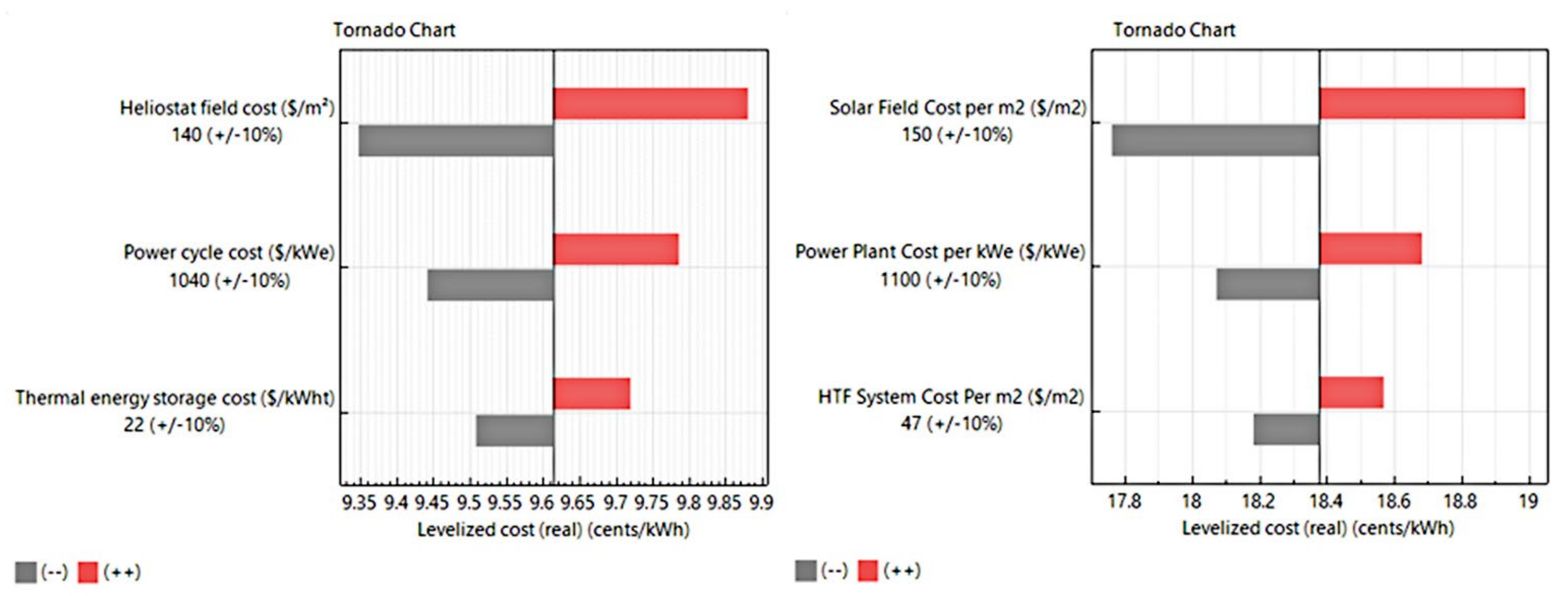
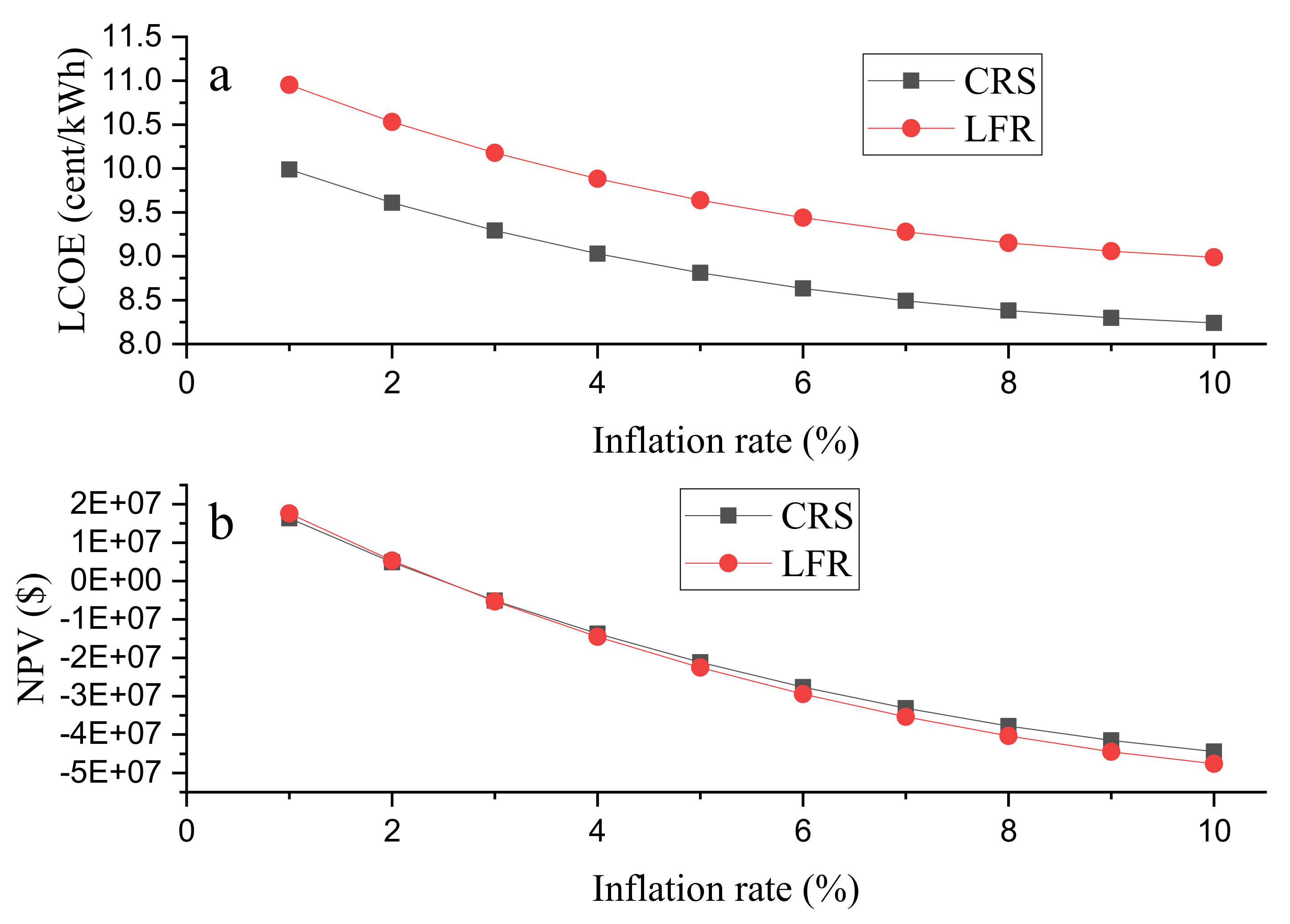
4.3.2. Economic Sensitivity Analysis

The discount rate is a critical input parameter that plays a role in determining the bankability of power plants. It considers the time value of the money invested and the risks of the investment. This study used a discount rate of 10% for both systems. To evaluate the impact of this factor on the bankability of both projects, a sensitivity analysis was done using discount values that range from 1% to 15%. Figure 10 shows the impact of the real discount rate on both technologies’ cost-effectiveness. As expected, the LCOE increases with increasing the real discount rate for both systems. However, the viability of the two different projects is significantly affected by the discount rate. A real discount rate above 9% renders both projects economically ineffective since the NPV for the two projects turns negative. Therefore, it suggests that the enormous DNI resource available at the selected site alone is not enough to make the projects bankable; the terms and conditions for financing the projects will have to be critically looked at and fashioned to support its development.

The effect of heliostat field cost, power cycle cost, TES cost, solar field cost, and HTF system cost on the LCOE for the two systems are presented in Figure 11. Data from the figure suggests that uncertainties in the heliostat and solar field cost significantly affect the LCOE. This is because the solar and heliostat fields form the most expensive components of the CSP technology [39,49]. Therefore, any uncertainty in their cost will affect the LCOE.

The increase in prices of goods and services within a particular time frame is defined as inflation. It is used to assess the level of loss in the value of money over a certain period [5]. The effect of the inflation rate on the two simulated projects is presented in Figure 12. As expected, the LCOE decreases with increasing inflation rate; however, the NPV can only be positive with a maximum inflation rate of 2%. An inflation rate above 2% renders the two systems economically impracticable to invest in since the NPV obtained is negative for both power plants.

Comparing the results obtained from the simulations, the CRS technology produced the highest monthly energy at the highest CF. The LFR generated less monthly energy at lower CF with higher LCOE. The relative differences in performance parameters between the two technologies (i.e., CRS and LFR) can be associated with the low concentration ratio and lower efficiency of the LFR technology, while the reverse can be applied to the CRS. The simulation suggests that the CRS system will be the best technological option for electricity generation at the selected site. Comparing the results obtained from the simulation to results of other literatures reviewed in Section 1, it can be observed that the results in this study fall within other obtained results and also close to the global weighted average of 0.108 $/kWh reported by IRENA in Reference [48] for the year 2020.

5. Conclusions

Ethiopia is located in the Eastern part of Africa with enormous solar energy potential, which is yet to be fully developed on a large scale to generate electricity to support the country’s electricity needs. This study investigated the technical and economic potential of two different technologies of CSP (i.e., LFR and CRS) for the Ethiopian electricity market. The two systems were modeled at a location known as Jijiga, one of the country’s places with high annual DNI. The study identified some important technical and financial information for developing the two systems through an optimization analysis. The SM for all TES scenarios in this study for the LFR is dependent on the TES period, while that of the CRS generally ranges between 1.5 and 2.0. The results also indicate that increasing/decreasing an SM increases/decreases the capacity factor, annual energy production, gross to net conversion factor, and the electricity source—power cycle gross output for both power plants. The LFR recorded annual energy of 528 TWh at a CF of 60.3%. The CRS also produced 540 TWh energy in year one at a CF of 61.9%. The maximum energy is generated in the dry seasons. Data from the figure suggests that uncertainties in the heliostat and solar field cost significantly affect the LCOE.

Moreover, it had been found that a discount and inflation rate above 9% and 2%, respectively, makes both technologies economically unviable. Therefore, the Ethiopian government and other governments in East Africa with similar CSP potentials must create an enabling financial environment to make such projects bankable. This can be in the form of tax waivers, incentives, and the reduction of interest rates on loans acquired by the private sector for such investments.

References

1. Winkler, B.; Lemke, S.; Ritter, J.; Lewandowski, I. Integrated assessment of renewable energy potential: Approach and application in rural South Africa. Environ. Innov. Soc. Transit. 2017, 24, 17–31. [Google Scholar] [CrossRef]
2. Agyekum, E.B. Energy poverty in energy rich Ghana: A SWOT analytical approach for the development of Ghana’s renewable energy. Sustain. Energy Technol. Assess. 2020, 40, 100760. [Google Scholar] [CrossRef]
3. Agyekum, E.B.; Velkin, V.I.; Hossain, I. Comparative evaluation of renewable energy scenario in Ghana. In IOP Conference Series: Materials Science and Engineering; IOP Publishing: Bristol, UK, 2019; p. 012157. [Google Scholar] [CrossRef]
4. Pueyo, A. What constrains renewable energy investment in Sub-Saharan Africa? A comparison of Kenya and Ghana. World Dev. 2018, 109, 85–100. [Google Scholar] [CrossRef]
5. Agyekum, E.B.; Nutakor, C. Feasibility study and economic analysis of stand-alone hybrid energy system for southern Ghana. Sustain. Energy Technol. Assess. 2020, 39, 100695. [Google Scholar] [CrossRef]
6. Ikejemba, E.C.; Schuur, P.C.; Van Hillegersberg, J.; Mpuan, P.B. Failures & generic recommendations towards the sustainable management of renewable energy projects in Sub-Saharan Africa (Part 2 of 2). Renew. Energy 2017, 113, 639–647. [Google Scholar]
7. Sweerts, B.; Longa, F.D.; van der Zwaan, B. Financial de-risking to unlock Africa’s renewable energy potential. Renew. Sustain. Energy Rev. 2019, 102, 75–82. [Google Scholar] [CrossRef]
8. Fritsch, A.; Frantz, C.; Uhlig, R. Techno-economic analysis of solar thermal power plants using liquid sodium as heat transfer fluid. Sol. Energy 2019, 177, 155–162. [Google Scholar] [CrossRef] [Green Version]
9. International Renewable Energy Agency (IRENA). Cost Analysis of Concentrating Solar Power 1 (2012). Available online: https://www.irena.org/documentdownloads/publications/re_technologies_cost_analysis-csp.pdf (accessed on 12 June 2020).
10. Elmohlawy, A.E.; Ochkov, V.F.; Kazandzhan, B.I. Thermal performance analysis of a concentrated solar power system (CSP) integrated with natural gas combined cycle (NGCC) power plant. Case Stud. Therm. Eng. 2019, 14, 100458. [Google Scholar] [CrossRef]
11. Dersch, J.; Geyer, M.; Herrmann, U.; Jones, S.A.; Kelly, B.; Kistner, R.; Ortmanns, W.; Pitz-Paal, R.; Price, H. Trough integration into power plants—a study on the performance and economy of integrated solar combined cycle systems. Energy 2004, 29, 947–959. [Google Scholar] [CrossRef]
12. Rashid, K.; Mohammadi, K.; Powell, K. Dynamic simulation and techno-economic analysis of a concentrated solar power (CSP) plant hybridized with both thermal energy storage and natural gas. J. Clean. Prod. 2020, 248, 119193. [Google Scholar] [CrossRef]
13. Islam, M.T.; Huda, N.; Saidur, R. Current energy mix and techno-economic analysis of concentrating solar power (CSP) technologies in Malaysia. Renew. Energy 2019, 140, 789–806. [Google Scholar] [CrossRef]
14. Aly, A.; Bernardos, A.; Fernandez-Peruchena, C.M.; Jensen, S.S.; Pedersen, A.B. Is Concentrated Solar Power (CSP) a feasible option for Sub-Saharan Africa?: Investigating the techno-economic feasibility of CSP in Tanzania. Renew. Energy 2019, 135, 1224–1240. [Google Scholar] [CrossRef]
15. Abaza, M.A.; El-Maghlany, W.M.; Hassab, M.; Abulfotuh, F. 10 MW Concentrated Solar Power (CSP) plant operated by 100% solar energy: Sizing and techno-economic optimization. Alex. Eng. J. 2020, 59, 39–47. [Google Scholar] [CrossRef]
16. Agyekum, E.B.; Velkin, V.I. Optimization and techno-economic assessment of concentrated solar power (CSP) in South-Western Africa: A case study on Ghana. Sustain. Energy Technol. Assess. 2020, 40, 100763. [Google Scholar] [CrossRef]
17. Zayed, M.E.; Zhao, J.; Li, W.; Elsheikh, A.H.; Zhao, Z.; Khalil, A.; Li, H. Performance prediction and techno-economic analysis of solar dish/stirling system for electricity generation. Appl. Therm. Eng. 2020, 164, 114427. [Google Scholar] [CrossRef]
18. Boukelia, T.E.; Mecibah, M.S.; Kumar, B.N.; Reddy, K.S. Optimization, selection and feasibility study of solar parabolic trough power plants for Algerian conditions. Energy Convers. Manag. 2015, 101, 450–459. [Google Scholar] [CrossRef]
19. Trabelsi, S.E.; Chargui, R.; Qoaider, L.; Liqreina, A.; Guizani, A. Techno-economic performance of concentrating solar power plants under the climatic conditions of the southern region of Tunisia. Energy Convers. Manag. 2016, 119, 203–214. [Google Scholar] [CrossRef]
20. Belgasim, B.; Aldali, Y.; Abdunnabi, M.J.; Hashem, G.; Hossin, K. The potential of concentrating solar power (CSP) for electricity generation in Libya. Renew. Sustain. Energy Rev. 2018, 90, 1–5. [Google Scholar] [CrossRef]
21. Agyekum, E.B.; Adebayo, T.S.; Bekun, F.V.; Kumar, N.M.; Panjwani, M.K. Effect of Two Different Heat Transfer Fluids on the Performance of Solar Tower CSP by Comparing Recompression Supercritical CO2 and Rankine Power Cycles, China. Energies 2021, 14, 3426. [Google Scholar] [CrossRef]
22. Guta, D.D. Determinants of household use of energy-efficient and renewable energy technologies in rural Ethiopia. Technol. Soc. 2020, 12, 101249. [Google Scholar] [CrossRef]
23. Guta, D.D. Effect of fuelwood scarcity and socio-economic factors on household bio-based energy use and energy substitution in rural Ethiopia. Energy Policy 2014, 75, 217–227. [Google Scholar] [CrossRef]
24. Global Solar Atlas. Available online: https://globalsolaratlas.info/download/ethiopia (accessed on 17 June 2020).
25. Kumar, V.; Shrivastava, R.L.; Untawale, S.P. Fresnel lens: A promising alternative of reflectors in concentrated solar power. Renew. Sustain. Energy Rev. 2015, 44, 376–390. [Google Scholar] [CrossRef]
26. Nate, N.; DiOrio, N.; Freeman, J.; Gilman, P.; Janzou, S.; Neises, T.; Wagner, M. System Advisor Model (SAM) General Description; Version 2017.9.5; National Renewable Energy Laboratory: Golden, CO, USA, 2018. Available online: https://www.nrel.gov/docs/fy18osti/70414.pdf (accessed on 25 June 2020).
27. Ezeanya, E.K.; Massiha, G.H.; Simon, W.E.; Raush, J.R.; Chambers, T.L. System advisor model (SAM) simulation modelling of a concentrating solar thermal power plant with comparison to actual performance data. Cogent Eng. 2018, 5, 1524051. [Google Scholar] [CrossRef]
28. Shafiee, M.; Alghamdi, A.; Sansom, C.; Hart, P.; Encinas-Oropesa, A. A Through-Life Cost Analysis Model to Support Investment Decision-Making in Concentrated Solar Power Projects. Energies 2020, 13, 1553. [Google Scholar] [CrossRef] [Green Version]
29. Photovoltaic Geographical Information System. Available online: https://re.jrc.ec.europa.eu/pvg_tools/en/tools.html#TMY (accessed on 19 June 2020).
30. Sharma, A.; Sharma, M. Power & energy optimization in solar photovoltaic and concentrated solar power systems. In Proceedings of the 2017 IEEE PES Asia-Pacific Power and Energy Engineering Conference (APPEEC), Bangalore, India, 8–10 November 2017; IEEE: Piscataway Township, NI, USA, 2017. [Google Scholar] [CrossRef]
31. Schiller, S. Direct Measurement of the Multiple-Scattering of Solar Radiation. In Proceedings of the 1998 IEEE International Geoscience and Remote Sensing, Seattle, WA, USA, 6–10 July 1998; IEEE: Piscataway Township, NI, USA, 1998; Volume 3, pp. 1559–1561. [Google Scholar]
32. Weather in Ethiopia: Climate, Seasons, and Average Monthly Temperature. Available online: https://www.tripsavvy.com/ethiopia-weather-and-average-temperatures-4071422 (accessed on 19 June 2020).
33. Hernández-Moro, J.; Martinez-Duart, J.M. Analytical model for solar PV and CSP electricity costs: Present LCOE values and their future evolution. Renew. Sustain. Energy Rev. 2013, 20, 119–132. [Google Scholar] [CrossRef]
34. Awan, A.B.; Zubair, M.; Praveen, R.P.; Bhatti, A.R. Design and comparative analysis of photovoltaic and parabolic trough based CSP plants. Sol. Energy 2019, 183, 551–565. [Google Scholar] [CrossRef]
35. Kincaid, N.; Mungas, G.; Kramer, N.; Wagner, M.; Zhu, G. An optical performance comparison of three concentrating solar power collector designs in linear Fresnel, parabolic trough, and central receiver. Appl. Energy 2018, 231, 1109–1121. [Google Scholar] [CrossRef]
36. Awan, A.B.; Zubair, M.; Mouli, K.V. Design, optimization and performance comparison of solar tower and photovoltaic power plants. Energy 2020, 199, 117450. [Google Scholar] [CrossRef]
37. Bishoyi, D.; Sudhakar, K. Modeling and performance simulation of 100 MW LFR based solar thermal power plant in Udaipur India. Resour.-Effic. Technol. 2017, 3, 365–377. [Google Scholar] [CrossRef]
38. Agyekum, E.B.; Velkin, V.I.; Hossain, I. Sustainable energy: Is it nuclear or solar for African Countries? Case study on Ghana. Sustain. Energy Technol. Assess. 2020, 37, 100630. [Google Scholar] [CrossRef]
39. Soomro, M.I.; Kim, W.S. Performance and economic evaluation of linear Fresnel reflector plant integrated direct contact membrane distillation system. Renew. Energy 2018, 129, 561–569. [Google Scholar] [CrossRef]
40. Zhao, Z.Y.; Chen, Y.L.; Thomson, J.D. Levelized cost of energy modeling for concentrated solar power projects: A China study. Energy 2017, 120, 117–127. [Google Scholar] [CrossRef]
41. Ethiopia Personal Income Tax Rate. Available online: https://tradingeconomics.com/ethiopia/personal-income-tax-rate (accessed on 24 June 2021).
42. Abbas, M.; Aburideh, H.; Belgroun, Z.; Tigrine, Z.; Merzouk, N.K. Comparative study of two configurations of solar tower power for electricity generation in Algeria. Energy Procedia 2014, 62, 337–345. [Google Scholar] [CrossRef] [Green Version]
43. Turchi, C.S.; Heath, G.A. Molten Salt Power Tower Cost Model for the System Advisor Model (SAM); National Renewable Energy Laboratory (NREL): Golden, CO, USA, 2013.
44. System Advisor Model (SAM). Available online: https://sam.nrel.gov/images/web_page_files/sam-help-2020-2-29-r1.pdf (accessed on 24 June 2020).
45. What Does a Power Purchase Agreement Mean in the Utilities Sector? Available online: https://www.investopedia.com/ask/answers/071415/what-does-power-purchase-agreement-ppa-mean-utilities-sector.asp (accessed on 25 June 2020).
46. NREL. Available online: https://sam.nrel.gov/financial-models/utility-scale-ppa.html (accessed on 25 June 2020).
47. Ethiopia Electricity Prices. Available online: https://www.globalpetrolprices.com/Ethiopia/electricity_prices/ (accessed on 26 June 2020).
48. IRENA. Renewable Power Generation Costs in 2018; International Renewable Energy Agency: Abu Dhabi, United Arab Emirates, 2019; Available online: https://www.irena.org/-/media/Files/IRENA/Agency/Publication/2021/Jun/IRENA_Power_Generation_Costs_2020.pdf (accessed on 5 January 2022).
49. Kassem, A.; Al-Haddad, K.; Komljenovic, D. Concentrated solar thermal power in Saudi Arabia: Definition and simulation of alternative scenarios. Renew. Sustain. Energy Rev. 2017, 80, 75–91. [Google Scholar] [CrossRef]
Figure 1. DNI map of Ethiopia. Reproduced from [24].
Sustainability 14 01677 g001
Figure 2. Types of CSP technologies (a) DE, (b) PTC, (c) CRS, and (d) LFR [13] (Permission to reproduce granted by Elsevier).
Sustainability 14 01677 g002
Figure 3. Monthly beam DNI profile for the studied site.
Sustainability 14 01677 g003
Figure 4. Monthly electricity generated for the LFR.
Sustainability 14 01677 g004
Figure 5. Monthly electricity generated for the CRS.
Sustainability 14 01677 g005
Figure 6. LCOE of LFR under different TES periods.
Sustainability 14 01677 g006
Figure 7. LCOE of CRS under different TES periods.
Sustainability 14 01677 g007
Figure 8. Effect of uncertainties of SM on some performance parameters of LFR.
Sustainability 14 01677 g008
Figure 9. Effect of uncertainties of SM on some performance parameters on CRS.
Sustainability 14 01677 g009
Figure 10. Sensitivity analysis on the discount rate (a) LCOE (b) NPV.
Sustainability 14 01677 g010
Figure 11. The effect of uncertainties in some input parameters on the LCOE.
Sustainability 14 01677 g011
Figure 12. Sensitivity analysis (a) LCOE and (b) NPV on inflation rate.
Sustainability 14 01677 g012