Effective Hybrid Soft Computing Approach for Optimum Design of Shallow Foundations

Abstract

In this study, an effective intelligent system based on artificial neural networks (ANNs) and a modified rat swarm optimizer (MRSO) was developed to predict the ultimate bearing capacity of shallow foundations and their optimum design using the predicted bearing capacity value. To provide the neural network with adequate training and testing data, an extensive literature review was used to compile a database comprising 97 datasets retrieved from load tests both on large-scale and smaller-scale sized footings. To refine the network architecture, several trial and error experiments were performed using various numbers of neurons in the hidden layer. Accordingly, the optimal architecture of the ANN was 5 × 10 × 1. The performance and prediction capacity of the developed model were appraised using the root mean square error (RMSE) and correlation coefficient (R). According to the obtained results, the ANN model with a RMSE value equal to 0.0249 and R value equal to 0.9908 was a reliable, simple and valid computational model for estimating the load bearing capacity of footings. The developed ANN model was applied to a case study of spread footing optimization, and the results revealed that the proposed model is competent to provide better optimal solutions and to outperform traditional existing methods.

1. Introduction

A spread footing is a geotechnical structure that transfers loads to the soil immediately beneath it. It is one of the most significant and sensitive structural components, and thus it has received a lot of attention in recent studies. Structures’ functionality can be jeopardized unless the effective loads are successfully transmitted to the earth by a well-designed foundation. As a result, the proper design of shallow footings is paramount to ensure the resilience of the structures they support. Spread footing structures are widely used and they typically involve large volumes of materials in their construction. Therefore, economical design of these structures is essential. However, in most geotechnical engineering optimization problems, the objective function is discontinuous and has a large number of design variables. These difficulties and complexity in geotechnical engineering challenges, such as shallow foundations, pile optimization, and slope stability and liquefaction, have prompted concerted research to develop new optimization techniques and approaches for the solution of these problems [1,2,3].

The ultimate bearing capacity and control of foundation settlement are two requirements that must be met by every foundation design. The bearing capacity is the resistance of the foundation when maximum pressure is applied by the foundation to the soil without triggering shear failure in the soil. By taking into account these criteria, several models and techniques have been developed in laboratory and in situ experiments to evaluate the ultimate bearing capacity, such as the theories presented by Terzaghi, Meyerhof, Hansen, Vesic, and others [4].

For both square and rectangular footings, the ultimate bearing capacity is determined by the foundation size. As a result, in terms of behavior and stress distribution, laboratory-made miniature models of footings differ from real-world footings. Therefore, when using the results of extremely small-scale model footing tests instead of full-scale behaviors, caution should be taken. Testing the actual size footing is necessary to understand true soil-foundation behavior; nevertheless, this is a time-consuming, experimentally challenging and expensive procedure. As a result of the scale effect, a majority of researchers have only focused on small-scale foundations of various sizes in the laboratory to establish final bearing capacity [5]. In addition, researchers are attempting to evaluate reliable approaches for predicting ultimate bearing capacity based on load test data from real-size foundations as well as smaller-scale model footings. Because of the variability of soils and the limitations of laboratory and field testing, a better approach for estimating bearing capacity is necessary.

Artificial neural networks (ANNs), which simulate the structure and learning mechanism of biological neural networks, are one of the most common prediction methods. ANNs are a class of parallel processing structures that work together to solve problems using highly interconnected but simple computing units called neurons. This enables the evaluation of non-linear correlations between any of the soil and foundation characteristics, as well as provides faster and more accurate results than earlier techniques. ANNs have recently been used to solve a variety of geotechnical engineering applications such as bearing capacity estimation [6,7], rock burst hazard prediction in underground projects [8], slope stability evaluation [9,10,11], concrete compressive strength prediction [12], and estimation of rock modulus [13]. This suggests that ANNs can be utilized for forecasting as well as prediction of events by simulating exceedingly complex functions [14]. The training procedure is one of the most important aspects of neural networks. The goal of this approach is to find the best possible connection weights and biases to attain the minimal amount of the objective function, which can be specified as root mean squared error (RMSE) or sum of squared errors (SSE). Generally, training algorithms can be divided into two categories: classic deterministic and recent metaheuristic algorithms. Classic optimization algorithms based on mathematical concepts take a long time or may not obtain the optimum solution at all. To address the aforementioned drawback, in the previous couple of decades, several metaheuristic optimization algorithms have been developed and applied for training ANNs. Some of this research includes: application of genetic algorithms [15], particle swarm optimization [16] and imperialistic competitive algorithms [9]. Although metaheuristics methods can produce acceptable results, there is no algorithm that can outperform others in solving all optimization problems. As a result, research has been conducted in an effort to modify the original algorithms’ performance and efficiency in some aspects and to apply them to a specific application. [17,18,19,20,21,22].

Rat swarm optimizer (RSO) is a relatively new metaheuristic optimization approach developed by Dhiman in 2020 [23]. Compared with other metaheuristics, RSO has a simple concept and structure and does not have complicated mathematical functions. The RSO algorithm mimics the following and attacking performances of rats in nature. Like the other population-based techniques, RSO, without any information about the solution, utilizes random initialization to generate the candidate solutions. Compared to the other metaheuristics, RSO possesses several advantages. It has a very simple structure, a fast convergence rate, and can be easily understood and utilized. However, like other metaheuristic algorithms, RSO commonly suffers from getting trapped in local minima when the objective function is complex and includes a rather large number of variables.

This paper presents an effective modified version of the RSO algorithm to overcome the mentioned weaknesses and implements a new algorithm for the optimum design of spread footings. In addition, an ANN model is created and trained using the proposed, modified RSO for predicting the ultimate bearing capacity of spread footings.

2. Foundation Optimization

Reinforced spread footings, as a key geotechnical construction, must securely and reliably support the superstructure, maintain stability against excessive settlement and failure of the soil’s bearing capacity, and restrict concrete stresses. Aside from these design goals, spread footings must meet a number of requirements: it must have enough shear and moment capacities in both long and short dimensions, the foundation’s bearing capacity cannot be exceeded, and the steel reinforcement design must comply with all design codes.

Mathematically, the general form of a constraint optimization problem can be expressed as follows:

minimize f (X)
subject to
g_i(X) ≤ 0, I = 1, 2, …, p,
h_j(X) = 0, j = 1, 2, …, m,
X^L ≤ X ≤ X^U

(1)

where X is n dimensional vector of design variables, f (X) is the objective function, g(X) and h(X) are inequality and equality constraints, respectively. Boundary constraints, X^L and X^U, are two n-dimensional vectors containing the design variables’ lower and upper bounds, respectively.

In the problem of foundation optimization, it is required that the objective function, design constraint, and design variables be identified, as presented in the following sub-sections.

2.1. Objective Function

The total cost of spread footing construction is used as the objective function in this study, and it may be represented mathematically as follows:

$$f\left(X\right)=C_c{V}_c+C_e{V}_e+C_b{V}_b+C_f{A}_f+C_s{W}_s$$

(2)

In Equation (2), C_c, C_e, C_b, C_f and C_s are the unit cost of concrete, excavation, backfill, formwork, and reinforcement, respectively.

Table 1. Unit cost of spread footing construction [24].

Item	Unit	Unit Cost (Euros)
Excavation	m3	25.16
Formwork	m2	51.97
Reinforcement	kg	2.16
Concrete	m3	173.96
Compacted backfill	m3	3.97

shows the unit expenses that are being considered [24].

2.2. Design Variables

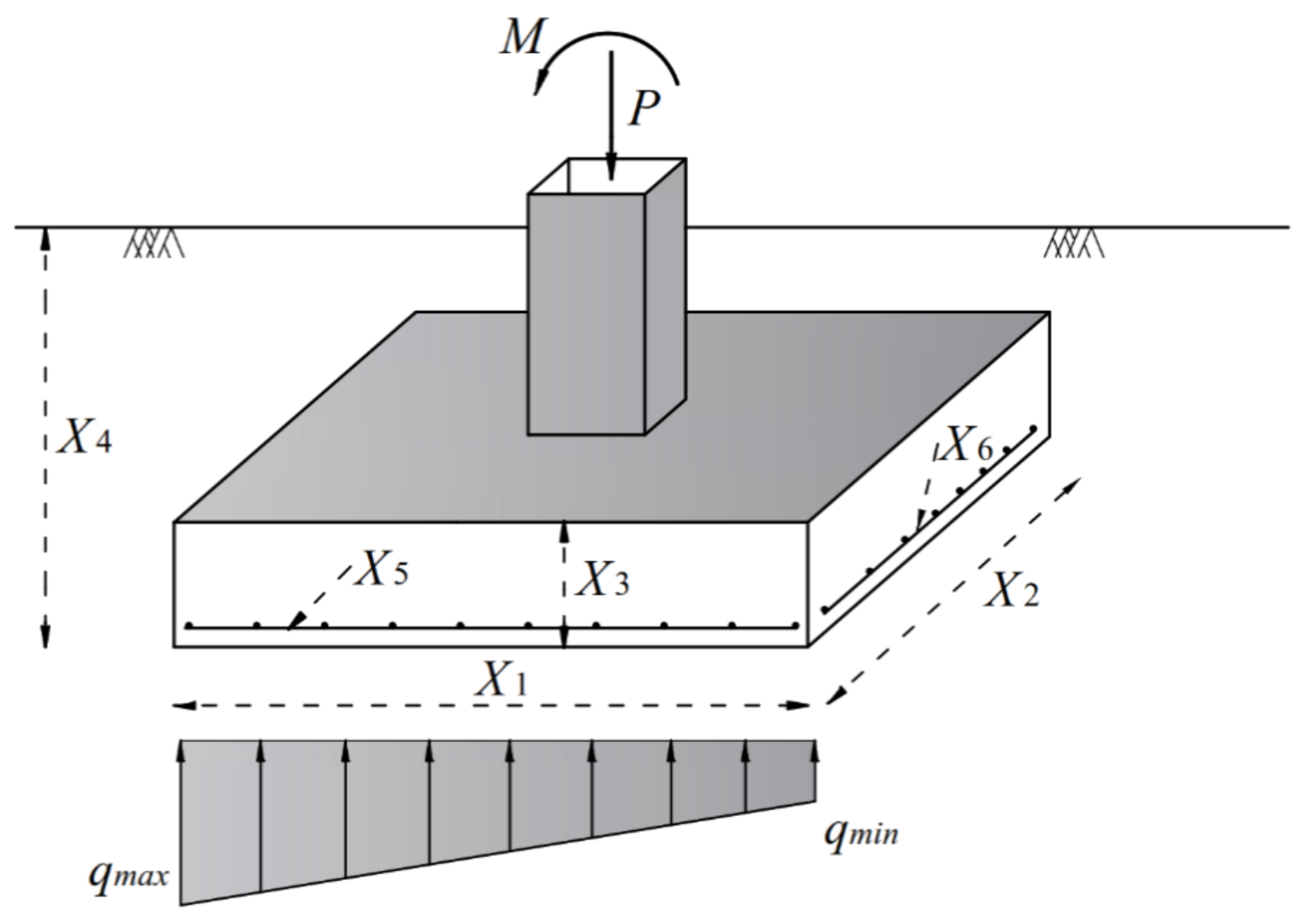
The design factors for the spread footing model are shown in Figure 1. There are two types of design variables: those that define geometrical parameters and those that describe reinforcing steel. The dimensions of the foundation are represented by four geometric design variables, as illustrated in Figure 1. X₁ is the foundation’s length, X₂ is the foundation’s width, X₃ is the foundation’s thickness and X₄ is the depth of embedment. Moreover, the steel reinforcement has two design variables: X₅ is the longitudinal reinforcement and X₆ is the transverse reinforcement.

2.3. Design Constraints

The forces operating on the footing are depicted in Figure 1. M and P denote the axial load and moment imparted to the footing in this figure. The minimum and maximum bearing pressures on the foundation’s base are q_min and q_max, respectively. The next sub-sections go over the design restrictions that must be taken into account when optimizing the spread footing.

Bearing capacity: The foundation’s bearing capacity must be sufficient to withstand the forces acting along the base. The maximum stress should be less than the soil’s bearing capacity to ensure a safe design:

$$q_{\max }\le \frac{q_{ult}}{F{S}_{}}$$

(3)

where q_ult denotes the foundation’s ultimate bearing capacity and q_max is the maximum contact pressure at the boundary between the foundation’s bottom and the underlying soil. In this study, an ANN model is established to estimate the q_ult in Section 6.

The lowest and highest applied bearing pressures on the foundation’s base are calculated as follows:

$$q_{\begin{array}{l}\min \\ \max \end{array}}=\frac{P}{X_1{X}_2}\left(1\pm \frac{6\hspace{0.17em}e}{X_1}\right)$$

(4)

where e denotes the eccentricity, which is defined as the ratio of the overturning moments (M) to the total vertical forces (P).

Eccentricity: The following requirements must be met such that tensile forces at the bottom of the footing are avoided:

$$e\le \frac{X_1}{6}$$

(5)

Settlement: According to the following inequalities, foundation settlement should be kept within a legal range:

$$\delta \le {\delta }_{all}$$

(6)

where δ_all is the permitted settlement and δ is the foundation’s immediate settlement. The settlement can be estimated as follows using the elastic solution proposed by Poulos and Davis [25]:

$$\delta =\frac{P(1-{\nu }^2)}{{\kappa }_{z}E\sqrt{X_1{X}_2}}$$

(7)

where κ_z is the shape factor, ν is the Poisson ratio and E is modulus of elasticity. In this research, the shape factor proposed by Wang and Kulhawy [24] is used as follows:

$${\kappa }_z=-0.0017{(X_2/X_1)}^2+0.0597(X_2/X_1)+0.9843$$

(8)

One-way shear: The footing must be viewed as a wide beam for one-way shear. According to ACI [26], the shear strength of concrete measured along a vertical plane extending the whole width of the base and located at a distance equal to the effective depth of the footing (V_u) should be less than the nominal shear strength of concrete:

$$V_u\le \frac{1}{6}{\varphi }_{\hspace{0.17em}V}\sqrt{f{\prime }_c}bd$$

(9)

where φ_V is the shear strength reduction factor of 0.75 [26], f′_c is the concrete compression strength, and b is the section width.

Two-way shear: The tendency of the column to punch through the footing slab is called punching shear. According to Equation (10), the maximum shearing force in the upward direction (V_u) should be less than the nominal punching shear strength to avoid such a failure.

$$V_u\le min\left\{(1+\frac{2}{{\beta }_c})/6,\left(\frac{{\alpha }_{s }d}{b_0}+2\right)/12,\frac{1}{3}\right\}{\varphi }_V\sqrt{f{’}_c}{b}_{0}d$$

(10)

where b₀ is the crucial section’s perimeter taken at d/2 from the column’s face, d denotes the depth at which steel reinforcement is placed, β_c is the ratio of a column section’s long side to its short side and α_s is equal to 40 for interior columns.

Bending moment: The nominal flexural strength of the reinforced concrete foundation section should be less than the moment capacity [26]:

$$M_u\le {\varphi }_M{A}_S{f}_y\left(d-\frac{a}{2}\right)$$

(11)

where M_u denotes the bending moment of the reaction stresses due to the applied load at the column’s face, φ_M presents the flexure strength reduction factor equal to 0.9 [26], A_s denotes the area of steel reinforcement and f_y is the yield strength of steel.

Reinforcements limitation: In each direction of the footing, the amount of steel reinforcement must fulfill minimum and maximum reinforcement area limitations according to the following inequality [26]:

$${\rho }_{\min }bd\le A_S\le {\rho }_{\max }bd$$

(12)

where A_S is the cross section of steel reinforcement, ρ_min and ρ_max are the minimum and maximum reinforcement ratios based on the following equations [26]:

$${\rho }_{\min }=\max \left\{\frac{1.4}{f_y},0.25\frac{\sqrt{{f^{\prime }}_c}}{f_y}\right\}$$

(13)

$${\rho }_{\max }=0.85{\beta }_1\frac{{f^{\prime }}_c}{f_y}\left(\frac{600}{600+f_y}\right)$$

(14)

Limitation of embedment’s depth: The depth of embedment should be limited between 0.5 and 2. Therefore:

$$0.5\le X_4\le 2$$

(15)

To address the above-mentioned limitations and transform a constrained optimization to an unconstrained one, a penalty function method is used in this paper, according to:

$$F\left(X\right)=f\left(X\right)+r{\displaystyle \sum }_{i=1}^{p}max{\left\{0, g_i\left(X\right)\right\}}^l$$

(16)

where F(X) is the penalized objective function, f(X) is the problem’s original objective function in Equation (2) and r is a penalty factor.

3. Modified Rat Swarm Optimizer

Rat Swarm Optimizer (RSO) is a novel metaheuristic algorithm inspired by the following and attacking behaviors of rats [23]. Rats are regional animals that live in a swarm of both males and females. In many circumstances, the rats’ behavior is extremely aggressive, which may result in the death of several animals. In this approach, the following and aggressive actions of rats are mathematically modelled to perform optimization [23]. Similar to the other population-based optimization techniques, the rat swarm optimizer starts with a set of random solutions which represent the rat’s position in the search space. This random population is estimated repeatedly by an objective function and improved based on following and aggressive behaviors of rats. In the original version of the RSO technique, the initial positions of eligible solutions (rats’ positions) are determined randomly in the search space as follows:

$$x_i=x_{i min}+rand\times \left(x_{i max}-x_{i min}\right), i=1,2,\dots , N$$

(17)

where $x_{i min}$ and $x_{i max}$ are the ith variable’s lower and upper limits, respectively. Generally, rats follow the bait in a group through their social painful behavior. Mathematically, to describe this performance of rats, it is assumed that the greatest search agent has the knowledge of bait placement. Therefore, the other search agents can inform their locations with respect to the greatest search agent obtained until now. The following equation has been suggested to represent the attacking process of rats using bait and produce the rat’s updated next position [23]:

$${\overrightarrow{P}}_i\left(t+1\right)=\left|{\overrightarrow{P}}_r\left(t\right)-\overrightarrow{P}\right|$$

(18)

where, ${\overrightarrow{P}}_i\left(t+1\right)$ defines the updated positions of ith rats, ${\overrightarrow{P}}_r\left(t\right)$ is the best optimal solution founded so far and t denotes the iteration number. In the above equation, $\overrightarrow{P}$ can be obtained using Equation (19).

$$\overrightarrow{P}=A\times {\overrightarrow{P}}_i\left(t\right)+C\times ({\overrightarrow{P}}_r\left(t\right)-{\overrightarrow{P}}_i\left(t\right))$$

(19)

where, ${\overrightarrow{P}}_i\left(t\right)$ defnes the positions of ith rats, and parameters A and C are calculated as follows:

$$A=R-t\times \left(\frac{R}{t_{max}}\right) ,t=1,2,3,\dots , t_{max}$$

(20)

C = 2 × rand

(21)

The parameter R is a random number between [1,5], C is a random number between [0,2] [23]. t is the current iteration of optimization process and $t_{max}$ is the maximum number of iterations. Equation (18) updates the locations of search agents and saves the best solution. Even though the performance of RSO to obtain the global optima is better than other evolutionary algorithms like Moth-fame Optimization (MFO), Grey Wolf Optimizer (GWO), and Gravitational Search Algorithm (GSA) [23], the algorithm may face some difficulty in finding better results through exploring complex functions.

To increase the performance and efficiency of RSO, this research presents a modified version of the algorithm using the idea of opposition-based learning (OBL). As mentioned before, RSO, as a member of population-based optimization algorithms, starts with a set of initial solutions and tries to improve performance toward the best solution. In the absence of a priori knowledge about the solution, the random initialization method is used to generate candidate solutions (rat’s initial positions) based on Equation (17). Obviously, the performance and convergence speed are directly related to the distance of the initial solutions from the best solution. In other words, the algorithm has a better performance if the randomly generated solutions have a lower value than the objective function. According to this idea and in order to improve the convergence speed and chance of finding the global optima of the standard RSO, this paper proposes a modified version of the algorithm called modified rat swarm optimization (MRSO). In the new MRSO, in the first iteration of the algorithm after generating the initial random solutions (i.e., rats’ positions) using Equation (17), the opposite positions of each solution will be generated based on the concept of opposite number. To describe the new population initialization, it is required to define the concept of opposite number. Let’s consider an N-dimensional vector X as follows:

X = (x₁, x₂, …, x_N)

(22)

where x_i ∈ [$x_{i min},x_{i max}$]. Then, the opposite point of $x_i$, which denoted by $\overline{x_i}$, is defined by:

$${\overline{x}}_i=\left(x_{i max}+x_{i min}\right)-x_{i }, i=1,2,\dots , N$$

(23)

To apply the concept of the opposite number in the population initialization of the MRSO, consider x_i to be a randomly generated solution in N-dimensional problems space (i.e., candidate solution). For this random solution, its opposite will be generated using Equation (23) and denoted by $\overline{x_i}$. Then, both solutions (i.e., x_i and $\overline{x_i}$) will be evaluated by the objective function f (.). Therefore, if f ($\overline{x_i}$) is better than f (x_i) (i.e., f ($\overline{x_i}$) < f (x_i)), the agent x_i will be replaced by $\overline{x_i}$; otherwise, we continue with x_i. Hence, in the first iteration, the initial solution and its opposite are evaluated simultaneously to continue with better (fitter) starting agents.

Despite the fact that MRSO is capable of expressing an efficient performance when compared to the traditional method, it can still get stuck in local optima and is not ideal for extremely difficult problems. In other words, during the search process, occasionally some agents fall into a local minimum and do not move for several iterations. To overcome these weaknesses and to increase the exploration and search capability, in the proposed MRSO at each iteration, the worst solution yielding the largest fitness value (in minimization problems) is replaced by a new solution according to the following equation:

$$x_{worst}=\left\{\begin{array}{c}ran{d}_1\times {\overrightarrow{P}}_r\left(t\right) if ran{d}_3\le 0.5\\ \left(x_{i max}+x_{i min}\right)-x_{i } if ran{d}_3>0.5\end{array}\right.$$

(24)

where, $x_{worst}$ is the solution with the maximum value of the objective function, $ran{d}_1$, $ran{d}_2$ and $ran{d}_3$ are random numbers between 0 and 1. The new approach exchanges the position vector of a least ranked rat with its opposite or based on the best solution found so far (${\overrightarrow{P}}_r\left(t\right)$) in each generation. This process attempts to modify the result by preserving population diversity and exploring new locations across the problem search area.

In summary, the suggested MRSO algorithm’s phases are implemented as follows: first, the initial random solutions and their opposites are generated, and then these solutions are evaluated according to the objective function to start the algorithm with fitter (better) solutions. Second, the population updating phase is conducted by updating the current solutions and then these solutions are evaluated again to replace the worst solution with a new one. Algorithm 1 shows the pseudo code for the proposed MRSO.

Algorithm 1 Modified Rat Swarm Optimization.

Define algorithm parameters: N,${\mathit{t}}_{\mathit{m}\mathit{a}\mathit{x}}$ For i =1 to N         //generate initial population Initialize the rats’ position, ${\mathit{x}}_{\mathit{i}}$, using Equation (17) Evaluate opposite of rats’ position, $\overline{x_i}$, based on Equation (23) If f ($\overline{x_i}$) < f (xi) Replace ${\mathit{x}}_{\mathit{i}}$ with $\overline{x_i}$ End if End for Initialize parameters A, C, and R     //algorithm process Calculate the fitness value of each search agent ${\overrightarrow{\mathit{P}}}_{\mathit{r}}$ ←best search agent While t <${\mathit{t}}_{\mathit{m}\mathit{a}\mathit{x}}$             //rats’ movement For i =1 to N Update parameters A and C by Equations (20) and (21) Update the positions of search agents using Equation (18) Calculate the fitness value of each search agent If the search agent goes beyond the boundary limits adjust it End for Change the worst agent with a new one using Equation (24) Update best agent ${\overrightarrow{\mathit{P}}}_{\mathit{r}}$ t = t + 1 End While

4. Artificial Neural Network

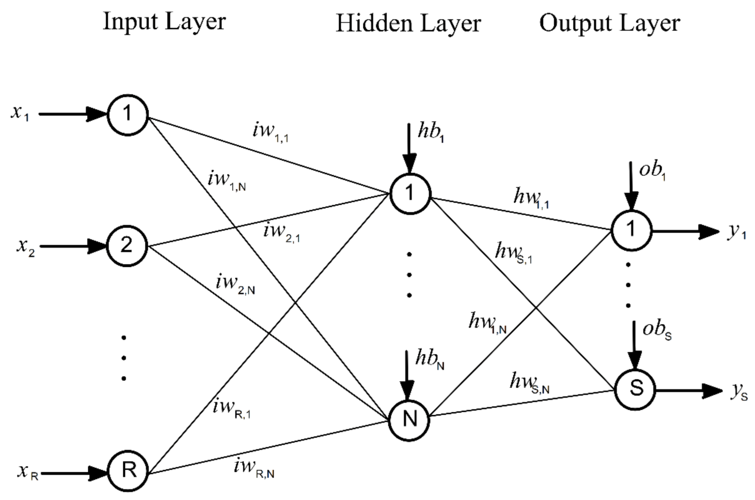
Artificial Neural Networks (ANNs) are parallel connectionist structures that are used to model the human brain’s functional network of neurons. ANNs are made up of neurons, which are extremely complicated mathematical processing units [27]. Weights and biases connect neurons. The input layer, hidden layer, and output layer all make up an ANN network [27]. Figure 2 illustrates a typical ANN model with one hidden layer. The input layer neurons receive data and transfer the data to the hidden layer, which conducts computation and sends the results to the last layer. The output layer is made up of neurons that send the system’s output to the user.

The number of hidden layers used in an ANN is determined by the complexity of the problem. If the network structure is small, it cannot reach a good level of effectiveness. Moreover, if it is too large, it will lead to redundant internal connections, loss of generalizability, and unnecessary complexity. According to the results of previous studies, one or two hidden layers are found to be sufficient and suitable for most situations and can solve any complex function [13,28]. The ANN models in this work are created using one hidden layer.

Furthermore, the most crucial task in the ANN architecture is determining neuron numbers in the hidden layer, which is dependent on the nature of the problem [13]. As suggested by Caudill [29], the number of neurons in the hidden layer required to map any function with R inputs has an upper limit of 2R+1.

In the network, the information passes from the input layer to the hidden layer and then to the output layer. As shown in Figure 2, in the presence of a bias, each neuron evaluates the sum of the weighted inputs and sends this sum through an activation function to generate the output. To get the optimum performance in training and testing, different transfer functions such as log-sigmoid and tan-sigmoid are examined. This process can be expressed as follows:

$$h{o}_j=f_j({{\displaystyle \sum }}_{i=1}^{R}i{w}_{j,i}{x}_i+h{b}_j)$$

(25)

where $i{w}_{j,i}$ is the weight connected between neurons i = (1, 2, …, R) and j = (1, 2, …, N), hb_j is a bias in hidden layer, R is the total number of neurons in the input layer, x_i is the corresponding input data and f is the transfer function.

In the output layer, the output of the neuron is obtained by the following equation:

$$y_k=f_k\left({{\displaystyle \sum }}_{j=1}^{N}h{w}_{k,j}h{o}_j+o{b}_k\right)$$

(26)

where $h{w}_{k,j}$ is the weight connected between neurons j = (1, 2, …, N) and k = (1, 2, …, S), $o{b}_k$ is a bias in output layer, N denotes the total number of neurons in the hidden layer, and S represents the total number of neurons in the output layer.

Following the formation of the ANN’s structure, training with known input and output data sets is carried out to determine the network’s appropriate weights and biases. The term “network training” refers to the process of determining the best values for the network’s weights and biases. Various techniques are typically used to determine the appropriate weights and biases for the ANN.

The ANN training is an unconstrained optimization problem involving the minimization of the global error by adjusting the values of synaptic weights and biases. A learning algorithm iteratively updates the values of the network parameters for provided training data, which consists of input–output vectors, to approach the target. This update procedure is commonly performed by back-propagating the error signal, layer by layer, and adjusting the parameters with respect to the magnitude of error signal. Back-propagation is the most widely utilized of various developed learning algorithms, and it has been used to represent many phenomena in the field of geotechnical engineering with considerable success. It requires less memory than the other algorithms and typically reaches an acceptable error level rapidly, although it can take a long time to converge properly on an error minimum. The network is trained by adjusting the weights and biases based on the differences between the actual and desired output values.

The prediction performance of the overall ANN model can be assessed by the correlation coefficient, R and the root mean squared error (RMSE). The coefficient of correlation is a measure that is used to determine the relative correlation and goodness-of-fit between the predicted and observed data. The following guide is suggested for values of R between 0.0 and 1.0 [30]:

R ≥ 0.8 strong correlation exists between two sets of variables;

0.2 < R < 0.8 correlation exists between the two sets of variables; and

R ≤ 0.2 weak correlation exists between the two sets of variables.

The RMSE is the most widely accepted measure of error and has the advantage that large errors receive much greater attention than small errors [29]. If R is 1.00 and RMSE is 0, the model’s predictive capability is treated as excellent. Therefore, a well-trained ANN model should have a R value near to 1 and low RMSE values.

The RMSE criteria is derived based on the neural network’s prediction of the training dataset, which can be obtained using the following equation:

$$RMSE=\sqrt{\frac{1}{M}{\displaystyle \sum }_{i=1}^M{\left(y-\widehat{y}\right)}^2}$$

(27)

where y and $\widehat{y}$ are the actual and the predicted values obtained by the model and M is total number of samples.

The ideal solution, which is considered as the weights and biases of the network associated with the minimized value of RMSE, is finally attained by continuous iterations. At the end of the training phase, the neurons’ associated trained weights and biases are stored in the network’s memory. The neural network is then tested using a different set of data in the next phase. In the testing phase, using the trained parameters, the network produces the target output values for the test data.

5. Performance Verification of MRSO

The effectiveness of the proposed method (MRSO) will be investigated in this section. On a set of benchmark test functions from the literature, the performance of MRSO is compared to that of the standard version of the algorithm (RSO) as well as some well-known metaheuristic algorithms. These are all minimization problems that can be used to evaluate new optimization algorithms’ robustness and search efficiency. The mathematical formula and characteristics of these test functions are shown in

Table 2. Benchmark functions’ details.

Function	Range	${\mathit{F}}_{\mathit{m}\mathit{i}\mathit{n}}$	n (Dim)	3D View
$F_1\left(X\right)={{\displaystyle \sum }}_{i=1}^n{x}_i^2$	${\left[-100, 100\right]}^n$	0	30
$F_2\left(X\right)={{\displaystyle \sum }}_{i=1}^n\left|x_i\right|+{{\displaystyle \prod }}_{i=1}^n\left|x_i\right|$	${\left[-10, 10\right]}^n$	0	30
$F_3\left(X\right)={{\displaystyle \sum }}_{i=1}^n{\left({{\displaystyle \sum }}_{j=1}^i{x}_j\right)}^2$	${\left[-100, 100\right]}^n$	0	30
$F_4\left(X\right)=\underset{i}{\max } \left\{\left|x_i\right|, 1\le i\le n \right\}$	${\left[-100, 100\right]}^n$	0	30
$F_5\left(X\right)={{\displaystyle \sum }}_{i=1}^{n-1}\left[100{\left(x_{i+1}-x_i^2\right)}^2+{\left(x_i-1\right)}^2\right]$	${\left[-30, 30\right]}^n$	0	30
$F_6\left(X\right)={{\displaystyle \sum }}_{i=1}^{n}i{x}_i^4+random\left[0,1\right)$	${\left[-1.28, 1.28\right]}^n$	0	30
$F_7\left(X\right)={{\displaystyle \sum }}_{i=1}^n-x_i\sin \left(\sqrt{\left|x_i\right|}\right)$	${\left[-500, 500\right]}^n$	428.9829 × n	30
$F_8\left(X\right)={{\displaystyle \sum }}_{i=1}^n\left[x_i^2-10\cos \left(2\pi x_i\right)+10\right]$	${\left[-5.12, 5.12\right]}^n$	0	30
$\begin{array}{cc}{F}_9\left(X\right)=-20 \exp & \left(-0.2\sqrt{\frac{1}{n}{{\displaystyle \sum }}_{i=1}^n{x}_i^2}\right)\hfill \\ & -exp\left(\frac{1}{n}{{\displaystyle \sum }}_{i=1}^n\cos \left(2\pi x_i\right)\right)+20\hfill \\ & +e\hfill \end{array}$	${\left[-32, 32\right]}^n$	0	30
$F_{10}\left(X\right)=\frac{1}{4000}{{\displaystyle \sum }}_{i=1}^n{x}_i^2-{{\displaystyle \prod }}_{i=1}^n\cos \left(\frac{x_i}{\sqrt{i}}\right)+1$	${\left[-600, 600\right]}^n$	0	30
$F_{11}\left(X\right)=$ $\begin{array}{cc}\frac{\pi }{n}\{10\sin \left(\pi y_1\right)& +{{\displaystyle \sum }}_{i=1}^{n-1}{\left(y_i-1\right)}^2[1\hfill \\ & +10{\sin }^2\left(\pi y_{i+1}\right)]+{\left(y_n-1\right)}^2\}\hfill \\ & +{{\displaystyle \sum }}_{i=1}^{n}u\left(x_i,10, 100, 4\right)\hfill \end{array}$ $\begin{array}{cc} y_i=& 1+\frac{x_{i+4}}{4}u\left(x_i,a, k, m\right)\hfill \\ & =\left\{\begin{array}{c}k{\left(x_i-a\right)}^m x_i>a \\ 0 a< x_i<a \\ k{\left(-x_i-a\right)}^m x_i<-a\end{array}\right.\hfill \end{array}$	${\left[-50, 50\right]}^n$	0	30
$\begin{array}{cc}{F}_{12}\left(X\right)=0.1\{{\sin }^2& \left(3\pi x_1\right)\hfill \\ & +{{\displaystyle \sum }}_{i=1}^n{\left(x_i-1\right)}^2[1\hfill \\ & +{\sin }^2\left(3\pi x_i+1\right)]\hfill \\ & +{\left(x_n-1\right)}^2\left[1+{\sin }^2\left(2\pi x_n\right)\right]\}\hfill \\ & +{{\displaystyle \sum }}_{i=1}^{n}u\left(x_i,5, 100, 4\right)\hfill \end{array}$	${\left[-50, 50\right]}^n$	0	30

.

The performance and robustness of the proposed MRSO are compared with the original RSO and some well-established optimization techniques, including Particle Swarm Optimization (PSO) [31], Moth-flame Optimization (MFO) [32] and Multi-Verse Optimizer (MVO) [33]. According to the literature [23] and to have a fair comparison between the selected methods, for all algorithms, the size of solutions (N) and maximum iteration number (t_max) are considered equal to 50 and 1000, respectively.

Because metaheuristics approaches are stochastic, a single run’s results may be incorrect. As a result, statistical analysis should be performed to provide a fair comparison and evaluate the effectiveness of the algorithms. To address this issue, 30 independent runs for the stated algorithms are performed, with the results presented in

Table 3. Comparison of different methods in solving test functions.

Function	Statistics	MRSO	RSO	PSO	MFO	MVO
F1	Mean	0.000	6.09 × 10−32	4.98 × 10−9	3.15 × 10−4	2.81 × 10−1
	Std.	0.000	5.67 × 10−35	1.40 × 10−8	5.99 × 10−4	1.11 × 10−1
F2	Mean	0.000	0.000	7.29 × 10−4	3.71 × 10+1	3.96 × 10−1
	Std.	0.000	0.000	1.84 × 10−3	2.16 × 10+1	1.41 × 10−1
F3	Mean	0.000	1.10 × 10−18	1.40 × 10	4.42 × 10+3	4.31 × 10
	Std.	0.000	4.47 × 10−19	7.13	3.71 × 10+3	8.97 × 10
F4	Mean	0.000	4.67 × 10−7	6.00 × 10−1	6.70 × 10	8.80 × 10−1
	Std.	0.000	1.96 × 10−8	1.72 × 10−1	1.06 × 10	2.50 × 10−1
F5	Mean	4.71 × 10−3	6.13	4.93 × 10	3.50 × 10+3	1.18 × 10+2
	Std.	0.000	7.97 × 10−1	3.89 × 10	3.98 × 10+3	1.43 × 10+2
F6	Mean	6.32 × 10−7	9.49 × 10−6	6.92 × 10−2	3.22 × 10−1	2.02 × 10−2
	Std.	4.75 × 10−7	1.83 × 10−5	2.87 × 10−2	2.93 × 10−1	7.43 × 10−3
F7	Mean	−1.25 × 10+4	−8.57 × 10+3	−6.01 × 10+3	−8.04 × 10+3	−6.92 × 10+3
	Std.	2.60	4.23 × 10+2	1.30 × 10+3	8.80 × 10+2	9.19 × 10+2
F8	Mean	0.000	1.57 × 10+2	4.72 × 10+1	1.63 × 10+2	1.01 × 10+2
	Std.	0.000	7.39 × 10	1.03 × 10	3.74 × 10	1.89 × 10
F9	Mean	8.88 × 10−16	7.40 × 10−17	3.86 × 10−2	1.60 × 10	1.15 × 10
	Std.	0.000	6.42	2.11 × 10−1	6.18 × 10	7.87 × 10−1
F10	Mean	0.000	0.000	5.50 × 10−3	5.03 × 10−2	5.74 × 10−1
	Std.	0.000	0.000	7.39 × 10−3	1.74 × 10−1	1.12 × 10−1
F11	Mean	2.90 × 10−3	5.52 × 10−1	1.05 × 10−2	1.26 × 10	1.27 × 10
	Std.	4.00 × 10−3	8.40	2.06 × 10−2	1.83 × 10	1.02 × 10
F12	Mean	2.15 × 10−2	6.05 × 10−2	4.03 × 10−1	7.24 × 10−1	6.60 × 10−1
	Std.	3.72 × 10−2	7.43 × 10−1	5.39 × 10−1	1.48 × 10	4.33 × 10−2

.

Table 3 shows that, when compared to conventional RSO and alternative optimization methods for all functions, MRSO can deliver better solutions in terms of the mean value of the objective functions. The results also reveal that the MRSO algorithm’s standard deviations are substantially smaller than those of the other techniques, indicating that the algorithm is stable. Based on the findings, it can be inferred that MRSO outperforms the standard algorithm as well as alternative optimization methods.

6. ANN for Prediction of Factor of Safety

In this section, an ANN model is developed and tested to forecast the shallow foundations’ ultimate bearing capacity. The determination of characteristics that affect bearing capacity is one of the more significant processes in model creation for bearing capacity estimation. Regardless of whether the values of bearing capacity produced using different traditional approaches vary significantly, the essential form of the equation is almost the same. The general form of the bearing capacity formula for foundations rested on cohesionless soil is presented in Equation (28).

$$q_{ult}=\gamma D{N}_q{S}_q{d}_q+0.5\gamma B{N}_{\gamma }{S}_{\gamma }{d}_{\gamma }$$

(28)

where γ is the unit weight of the soil, B denotes the width of the footing and D is the depth of soil above the foundation base. N_q and N_γ are bearing capacity factors that are dependent on the internal friction angle of the base soil, d_q and d_γ are depth factors, and s_q and s_γ are shape factors [4].

Several researchers have introduced different equations for the evaluation of these factors. The equations for bearing capacity factors, shape factors and depth factors based on Meyerhof’s theory are presented in the following equations:

$$N_q=e^{\pi tan\varnothing }ta{n}^2\left(45+\frac{\varnothing }{2}\right)$$

(29)

$$N_{\gamma }=\left(N_q-1\right)tan\left(1.4\varnothing \right)$$

(30)

$$s_q=s_{\gamma }=1+0.1ta{n}^2\left(45+\frac{\varnothing }{2}\right)\frac{B}{L}$$

(31)

$$d_q=d_{\gamma }=1+0.1ta{n}^2\left(45+\frac{\varnothing }{2}\right)\frac{D}{B}$$

(32)

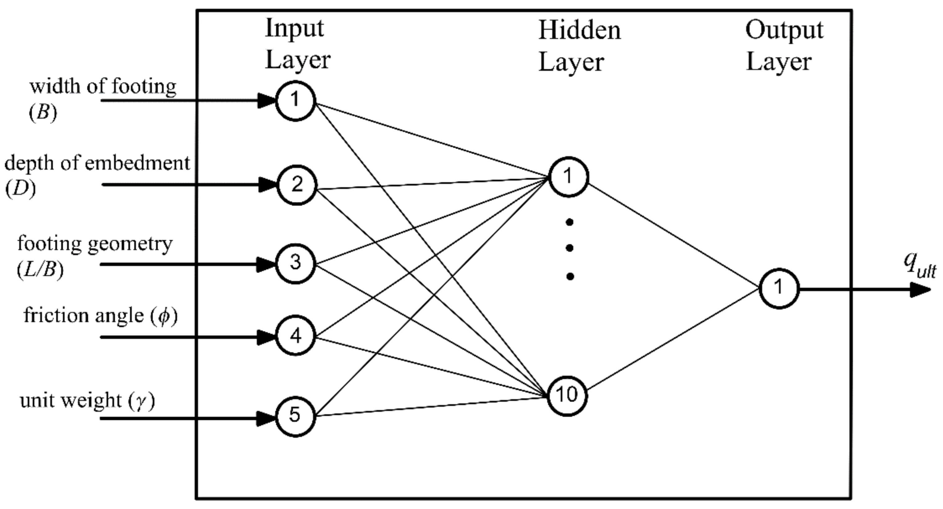
As shown in Equations (28)–(32), the bearing capacity of a foundation is governed by a range of physical characteristics of the foundation and the soil in which it is embedded. Among the variables related to the foundation geometry, the following are the primary elements influencing the bearing capacity: footing’s width (B), footing’s length (L), footing’s shape, and depth of embedment (D). In addition, the angle of shearing resistance of the soil (ϕ) and the unit weights (γ) are the most important parameters with regard to the soil that affect the bearing capacity. Based on the above, the five input parameters for the ANN model creation in this study include: footing’s width (B), depth of embedment (D), geometry of footing (L/B), soil’s unit weight (γ), and friction angle (ϕ). The single output variable of the ANN is the footing’s ultimate bearing capacity (q_ult). The proposed ANN model to predict the q_ult is shown in Figure 3.

The data for calibrating and validating the neural network model was gathered from prior experimental research in the literature, which included load test data on real-sized foundations, as well as the footing and soil information. There are 97 data sets in all, with 47 dealing with load tests on large-scale footings and 50 with lower scale model footings.

The data used are presented in Appendix A. These data were implemented for network training and validating.

Neural network training can be made more efficient, if an adequate normalization is performed for the network input and output variables previous to the training process. Normalizing the data generally eliminates variations in input and output parameters, speeds up learning, leads to faster convergence, and significantly reduces calculation time [34]. In the current study, before training, the following normalization expression is used to scale the input and output data to lie between −1 and 1.

$$X_{norm}=\frac{X-X_{min}}{X_{max}-X_{min}}$$

(33)

where X represents the measured value, X_norm is the normalized value of the measured parameter, X_min and X_max are the minimum and maximum values for the measured parameters. In the training process of the network, the available dataset is split into two sections: training and testing. The training data is used to adjust the network parameters and the testing data is used to verify the performance of the model. Usually, 80% of the data are suggested for model training and 20% for testing [35]. Accordingly, we randomly divided the dataset into training and testing sub-classes that have the respective amounts of 0.8 (i.e., 78 data sets) and 0.2 (i.e., 19 data sets).

An experimental investigation was used to identify the optimal number of neurons in the model’s hidden layer. In this experiment, the performance of the model (i.e., RMSE and R) was evaluated with a different number of neurons by considering tan-sigmoid as the transfer function. The network’s parameters were evaluated using both MRSO and RSO algorithms to minimize the error between the real and predicted values of q_ult. To compare the performance of these algorithms for training the network, 30 independent runs were conducted using both algorithms and the best values of the Root Mean Square Error (RMSE) and the correlation coefficient (R) for all training samples are collected and presented in

Table 4. Effects of different neurons numbers in predicting q_ult.

Neurons Number	Algorithm	RMSE	R
1	MRSO RSO	0.152 0.348	0.8043 0.7539
2	MRSO RSO	0.135 0.248	0.8275 0.7902
3	MRSO RSO	0.106 0.181	0.8910 0.8386
4	MRSO RSO	0.087 0.142	0.9102 0.8779
5	MRSO RSO	0.069 0.105	0.9444 0.8991
6	MRSO RSO	0.056 0.095	0.9505 0.9272
7	MRSO RSO	0.044 0.078	0.9727 0.9403
8	MRSO RSO	0.034 0.060	0.9828 0.9764
9	MRSO RSO	0.0291 0.0414	0.9888 0.9795
10	MRSO RSO	0.0289 0.0342	0.9908 0.9875
11	MRSO RSO	0.0314 0.0408	0.9817 0.9786

. From Table 4, it is shown that the optimum number of the neurons in the hidden layer is equal to 10. Moreover, the results indicate that the best values of RMSE and R obtained by MRSO are lower than those evaluated by RSO and the new algorithm apparently performs better than RSO in the model training.

Following determination of the model’s structure, the parameters of the ANN model (i.e., the connecting weights and biases) need to be determined. In this study, the proposed MRSO as an effective optimization algorithm was implemented to determine the weights and biases of the network associated with the minimum value of RMSE. Thereafter, using the trained parameters, the network produced the target output values (i.e., q_ult).

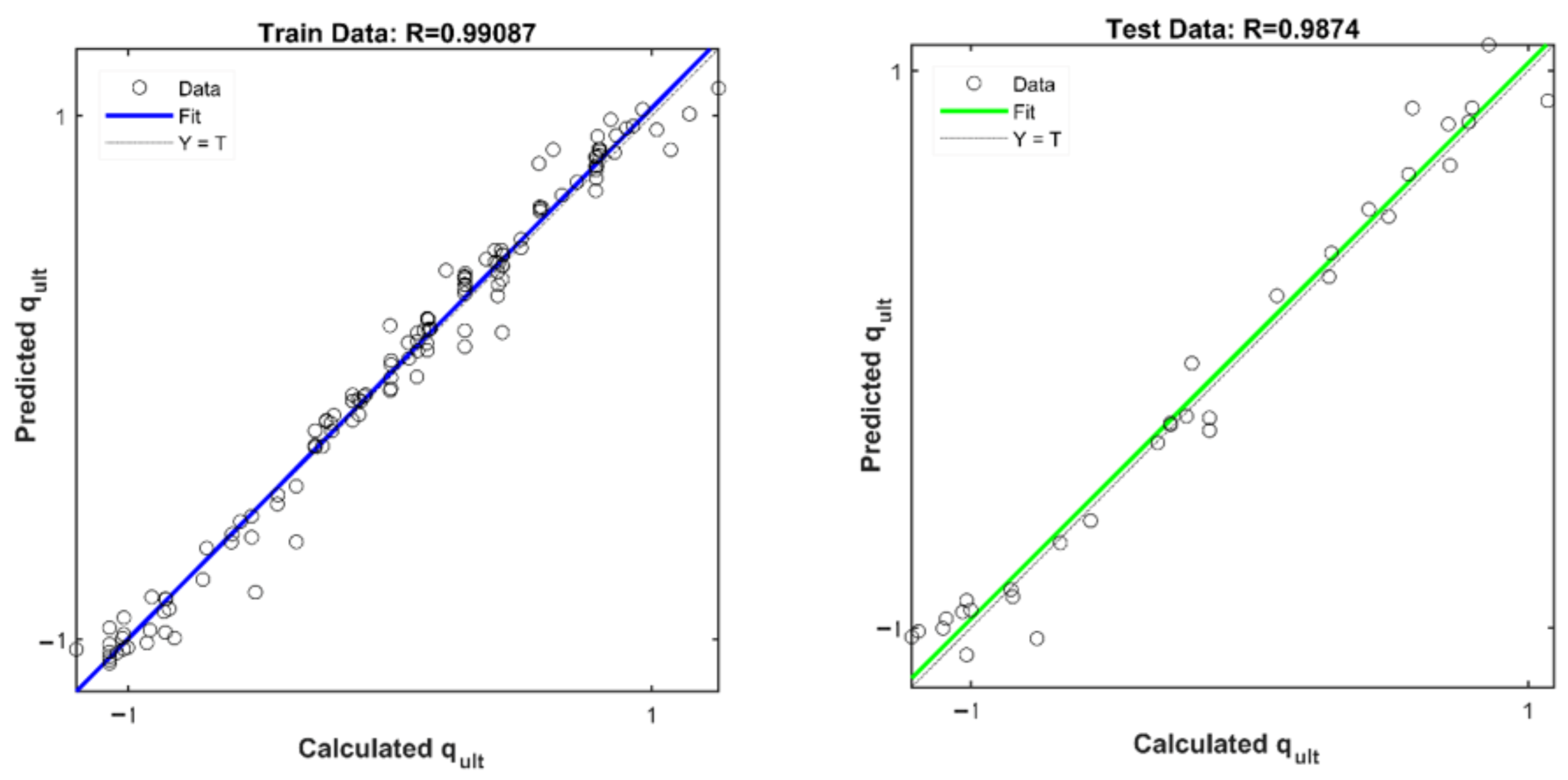
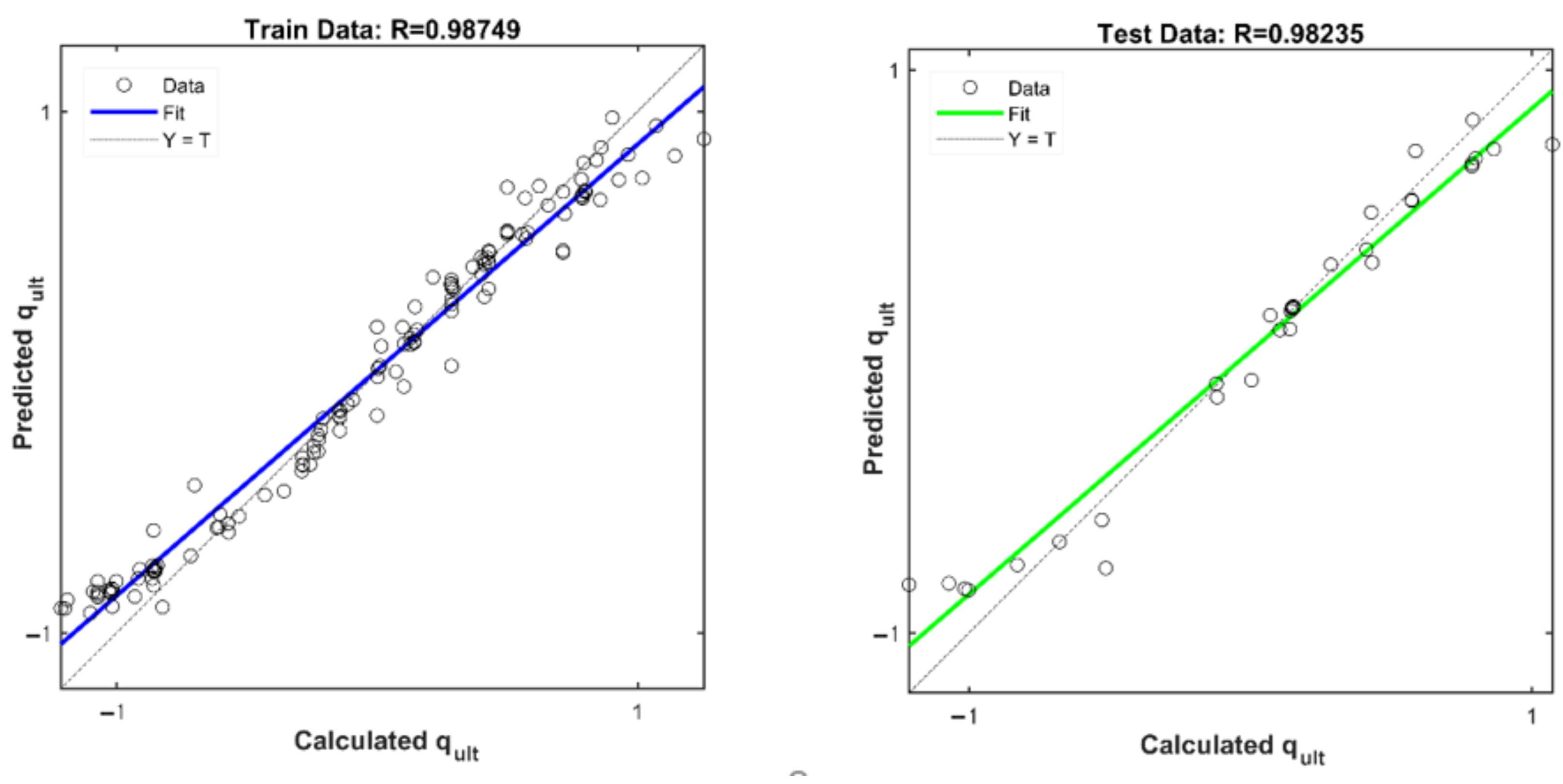
Figure 4 and Figure 5 display the actual values of q_ult together with their predicted values obtained by MRSO and RSO for training and testing datasets, respectively. According to these figures, the MRSO model can predict better results for both training and testing datasets and it can be introduced as a new hybrid model in this field.

In addition, to obtain a consistent data division of the developed model, several combinations of the training and testing sets are considered. This is to ensure the reliability and repeatability of the trained network when it comes to forecasting the testing dataset.

In this experiment, the data presented in Appendix A is partitioned into five groups. Each group is randomly split into two groups: the first group is used for training the neural network model, and the other (20% of the data set) for testing. Then, the mean value of the RMSEs obtained on five different testing subsets is estimated, which is equal to 0.0298 in this experiment. The results of this experiment could verify the reliability of the proposed model.

7. Model Application

In this section, the optimum design of an interior spread footing in dry sand is conducted using the proposed MRSO. This problem was solved previously by Khajehzadeh et al. [36] using the modified particle swarm optimization (MPSO) technique. Khajehzadeh et al. [36] applied Meyerhof’s method for evaluation of ultimate bearing capacity. However, in the current study, the ultimate bearing capacity is predicted using the developed ANN model based on in situ test results. Other input parameters for the case study are given in

Table 5. Input parameters for the case study.

Parameter	Unit	Value for Example
Effective friction angle of base soil	degree	30
Unit weight of base soil	kN/m3	18
Young’s modulus	MPa	35
Poisson’s ratio	−	0.3
Vertical load	kN	3480
Moment	kN m	840
Concrete cover	cm	7.0
Yield strength of reinforcing steel	MPa	400
Compressive strength of concrete	MPa	30
Factor of safety for bearing capacity	−	3.0
Allowable settlement of footing	m	0.04

.

The problem is solved by the presented procedure. In order to verify the efficiency of the proposed method, the analysis results are compared with the standard RSO as well as modified particle swarm optimization (MPSO). The best results of the analyses for the minimum cost are presented in

Table 6. Optimization result for spread footing optimization.

Design Variable	Unit	Optimum Values MRSO (Current Study)	Optimum Values RSO (Current Study)	Optimum Values MPSO [36]
X1	m	5.30	5.75	5.75
X2	m	1.90	1.82	1.70
X3	m	0.503	0.505	0.67
X4	m	1.90	1.82	1.70
X5	cm2	135	149.7	160
X6	cm2	25	23.1	23
Objective function	Euros	2756	2845	2926

.

The findings presented in Table 6 show that the optimum design evaluated by the proposed methodology in the current study using the ANN model and MRSO algorithm is lower than those evaluated by standard RSO and MPSO techniques. According to the results, the best price obtained by MRSO is 2756 USD, almost 3.2% lower than the best price calculated by RSO, which means the new method could provide a better solution. In addition, the difference between the best prices evaluated by the MRSO and MPSO is almost 6.2%, which indicates that the predicted ultimate bearing capacity using the proposed ANN model can provide acceptable results compared with the traditional methods for bearing capacity estimation.

8. Summary and Conclusions

In this research, an effective optimization method based on the rat swarm optimizer, namely modified rat swarm optimization (MRSO), was developed and applied for neural network training as well as optimal design of spread foundations. In the proposed modified RSO, both the initial random solutions and their opposites were evaluated in the first iteration of the algorithm, and if the opposite solution’s fitness was lower than the random one, the opposite solution would be selected. As a result, the algorithm begins with better solutions instead of random ones. Furthermore, the new algorithm replaces the worst solution with a better one at each iteration to improve the algorithm’s exploration capabilities as well as its performance and convergence rate. In addition, efforts were made to develop an ANN model that could be used to estimate the ultimate bearing capacity of shallow foundations on granular soil. To prepare a suitable database for the development of the ANN model, data was retrieved from 97 load tests on footings (with sizes that match to actual footings and smaller model footings) from the literature. After preparing the training database, the proposed MRSO algorithm was implemented for training the network model. Based on the obtained results of this study, the following conclusions can be drawn:

• The performance comparison of the proposed MRSO algorithm on a set of benchmark functions reveals that the MRSO outperforms the standard RSO and other algorithms.
• The most optimal network for q_ult estimation is a three-layer neural network with 10 neurons in the hidden layer.
• The developed ANN model can be applied for ultimate bearing capacity estimation with RMSE equal to 0.0249 and a correlation coefficient equal to 0.9908.
• The new MRSO algorithm was successfully applied to a case study of spread footing optimization from the literature.
• According to the numerical experiment, the MRSO algorithm outperforms the other methods and may provide a cheaper design for spread foundations.

References

- Kaveh, A.; Seddighian, M.R. Optimization of Slope Critical Surfaces Considering Seepage and Seismic Effects Using Finite Element Method and Five Meta-Heuristic Algorithms. Period. Polytech. Civ. Eng. 2021, 65, 425–436. [Google Scholar] [CrossRef]
- Chan, C.M.; Zhang, L.; Ng, J.T. Optimization of pile groups using hybrid genetic algorithms. J. Geotech. Geoenviron. Eng. 2009, 135, 497–505. [Google Scholar] [CrossRef]
- Gandomi, A.H.; Kashani, A.R. Construction cost minimization of shallow foundation using recent swarm intelligence techniques. IEEE Trans. Ind. Inform. 2017, 14, 1099–1106. [Google Scholar] [CrossRef]
- Das, B.M. Principles of Foundation Engineering; Cengage Learning: Boston, MA, USA, 2015. [Google Scholar]
- Taylor, R.E. Geotechnical Centrifuge Technology; CRC Press: London, UK, 2018. [Google Scholar]
- Ahmad, M.; Ahmad, F.; Wróblewski, P.; Al-Mansob, R.A.; Olczak, P.; Kamiński, P.; Safdar, M.; Rai, P. Prediction of Ultimate Bearing Capacity of Shallow Foundations on Cohesionless Soils: A Gaussian Process Regression Approach. Appl. Sci. 2021, 11, 10317. [Google Scholar] [CrossRef]
- Moayedi, H.; Moatamediyan, A.; Nguyen, H.; Bui, X.-N.; Bui, D.T.; Rashid, A.S.A. Prediction of ultimate bearing capacity through various novel evolutionary and neural network models. Eng. Comput. 2020, 36, 671–687. [Google Scholar] [CrossRef]
- Ahmad, M.; Hu, J.-L.; Hadzima-Nyarko, M.; Ahmad, F.; Tang, X.-W.; Rahman, Z.U.; Nawaz, A.; Abrar, M. Rockburst Hazard Prediction in Underground Projects Using Two Intelligent Classification Techniques: A Comparative Study. Symmetry 2021, 13, 632. [Google Scholar] [CrossRef]
- Gao, W.; Raftari, M.; Rashid, A.S.A.; Mu’azu, M.A.; Jusoh, W.A.W. A predictive model based on an optimized ANN combined with ICA for predicting the stability of slopes. Eng. Comput. 2020, 36, 325–344. [Google Scholar] [CrossRef]
- Khajehzadeh, M.; Taha, M.R.; Keawsawasvong, S.; Mirzaei, H.; Jebeli, M. An Effective Artificial Intelligence Approach for Slope Stability Evaluation. IEEE Access 2022, 10, 5660–5671. [Google Scholar] [CrossRef]
- Abdalla, J.A.; Attom, M.F.; Hawileh, R. Prediction of minimum factor of safety against slope failure in clayey soils using artificial neural network. Environ. Earth Sci. 2015, 73, 5463–5477. [Google Scholar] [CrossRef]
- Ahmad, M.; Hu, J.-L.; Ahmad, F.; Tang, X.-W.; Amjad, M.; Iqbal, M.J.; Asim, M.; Farooq, A. Supervised Learning Methods for Modeling Concrete Compressive Strength Prediction at High Temperature. Materials 2021, 14, 1983. [Google Scholar] [CrossRef]
- Sonmez, H.; Gokceoglu, C.; Nefeslioglu, H.; Kayabasi, A. Estimation of rock modulus: For intact rocks with an artificial neural network and for rock masses with a new empirical equation. Int. J. Rock Mech. Min. Sci. 2006, 43, 224–235. [Google Scholar] [CrossRef]
- Choobbasti, A.; Farrokhzad, F.; Barari, A. Prediction of slope stability using artificial neural network (case study: Noabad, Mazandaran, Iran). Arab. J. Geosci. 2009, 2, 311–319. [Google Scholar] [CrossRef]
- Wang, H.; Moayedi, H.; Kok Foong, L. Genetic algorithm hybridized with multilayer perceptron to have an economical slope stability design. Eng. Comput. 2021, 37, 3067–3078. [Google Scholar] [CrossRef]
- Rukhaiyar, S.; Alam, M.; Samadhiya, N. A PSO-ANN hybrid model for predicting factor of safety of slope. Int. J. Geotech. Eng. 2018, 12, 556–566. [Google Scholar] [CrossRef]
- Koessler, E.; Almomani, A. Hybrid particle swarm optimization and pattern search algorithm. Optim. Eng. 2021, 22, 1539–1555. [Google Scholar] [CrossRef]
- Gao, W. Modified ant colony optimization with improved tour construction and pheromone updating strategies for traveling salesman problem. Soft Comput. 2021, 25, 3263–3289. [Google Scholar] [CrossRef]
- Delice, Y.; Aydoğan, E.K.; Özcan, U.; İlkay, M.S. A modified particle swarm optimization algorithm to mixed-model two-sided assembly line balancing. J. Intell. Manuf. 2017, 28, 23–36. [Google Scholar] [CrossRef]
- Kiran, S.H.; Dash, S.S.; Subramani, C. Performance of two modified optimization techniques for power system voltage stability problems. Alex. Eng. J. 2016, 55, 2525–2530. [Google Scholar] [CrossRef] [Green Version]
- Khajehzadeh, M.; Taha, M.R.; El-Shafie, A.; Eslami, M. Search for critical failure surface in slope stability analysis by gravitational search algorithm. Int. J. Phys. Sci. 2011, 6, 5012–5021. [Google Scholar]
- Khajehzadeh, M.; Taha, M.R.; Eslami, M. Multi-objective optimization of foundation using global-local gravitational search algorithm. Struct. Eng. Mech. Int. J. 2014, 50, 257–273. [Google Scholar] [CrossRef]
- Dhiman, G.; Garg, M.; Nagar, A.; Kumar, V.; Dehghani, M. A novel algorithm for global optimization: Rat swarm optimizer. J. Ambient. Intell. Humaniz. Comput. 2021, 12, 8457–8482. [Google Scholar] [CrossRef]
- Wang, Y.; Kulhawy, F.H. Economic design optimization of foundations. J. Geotech. Geoenviron. Eng. 2008, 134, 1097–1105. [Google Scholar] [CrossRef]
- Poulos, H.G.; Davis, E.H. Elastic Solutions for Soil and Rock Mechanics; Wiley: New York, NY, USA, 1974. [Google Scholar]
- ACI 318-05Building Code Requirements for Structural Concrete and Commentary; American Concrete Institute International: Farmington Hills, MI, USA, 2005.
- Anderson, J.A. An Introduction to Neural Networks; MIT Press: Cambridge, MA, USA, 1995. [Google Scholar]
- Baheer, I. Selection of methodology for modeling hysteresis behavior of soils using neural networks. Comput.-Aided Civ. Infrastruct. Eng. 2000, 5, 445–463. [Google Scholar] [CrossRef]
- Caudill, M. Neural networks primer, Part III. AI Expert 1988, 3, 53–59. [Google Scholar]
- Smith, G.N. Probability and Statistics in Civil Engineering; Collins Professional and Technical Books: London, UK, 1986. [Google Scholar]
- Kennedy, J.; Eberhart, R. Particle swarm optimization. In Proceedings of the ICNN’95—International Conference on Neural Networks, Perth, Australia, 27 November–1 December 1995; pp. 1942–1948. [Google Scholar]
- Mirjalili, S. Moth-flame optimization algorithm: A novel nature-inspired heuristic paradigm. Knowl.-Based Syst. 2015, 89, 228–249. [Google Scholar] [CrossRef]
- Mirjalili, S.; Mirjalili, S.M.; Hatamlou, A. Multi-verse optimizer: A nature-inspired algorithm for global optimization. Neural Comput. Appl. 2016, 27, 495–513. [Google Scholar] [CrossRef]
- Sola, J.; Sevilla, J. Importance of input data normalization for the application of neural networks to complex industrial problems. IEEE Trans. Nucl. Sci. 1997, 44, 1464–1468. [Google Scholar] [CrossRef]
- Moayedi, H.; Abdullahi, M.a.M.; Nguyen, H.; Rashid, A.S.A. Comparison of dragonfly algorithm and Harris hawks optimization evolutionary data mining techniques for the assessment of bearing capacity of footings over two-layer foundation soils. Eng. Comput. 2021, 37, 437–447. [Google Scholar] [CrossRef]
- Khajehzadeh, M.; Taha, M.R.; El-Shafie, A.; Eslami, M. Modified particle swarm optimization for optimum design of spread footing and retaining wall. J. Zhejiang Univ. Sci. A 2011, 12, 415–427. [Google Scholar] [CrossRef]
- Muhs, H.; Elmiger, R.; Weiß, K. Sohlreibung und Grenztragfähigkeit Unter Lotrecht und Schräg Belasteten Einzelfundamenten; Deutsche Forschungsgesellschaft für Bodenmechanik (DEGEBO): Berlin, Germany, 1969. [Google Scholar]
- Weiß, K. Der Einfluß der Fundamentform auf die Grenztragfähigkeit Flachgegründeter Fundamente, Untersuchungen Ausgef von Klaus Weiß: Mit 14 Zahlentaf; Deutsche Forschungsgesellschaft für Bodenmechanik (DEGEBO): Berlin, Germany, 1970. [Google Scholar]
- Muhs, H.; Weiss, K. Untersuchung von Grenztragfähigkeit und Setzungsverhalten Flachgegründeter Einzelfundamente im Ungleichförmigennichtbindigen Boden; Deutsche Forschungsgesells chaft für Bodenmechanik (DEGEBO): Berlin, Germany, 1971. [Google Scholar]
- Muhs, H. Inclined load tests on shallow strip footings. In Proceedings of the 8th International Conference on Soil Mechanism and Foundation Engineering, Moscow, Russia, 6–11 August 1973; Volume II, pp. 173–179. [Google Scholar]
- Briaud, J.-L.; Gibbens, R. Behavior of five large spread footings in sand. J. Geotech. Geoenviron. Eng. 1999, 125, 787–796. [Google Scholar] [CrossRef]
- Gandhi, G. Study of Bearing Capacity Factors Developed from Lab. Experiments on Shallow Footings on Cohesionless Soils. Ph.D. Thesis, Shri GS Institute of Tech and Science, Indore, India, 2003. [Google Scholar]
Figure 1.
Design variables of the footing.
Figure 2.
Typical ANN model.
Figure 3.
Neural model for qult prediction.
Figure 4.
Relationship between real and predicted qult from the ANN model trained by MRSO.
Figure 5.
Relationship between real and predicted qult from the ANN model trained by RSO.