Article

A Multi-Scenario Simulation and Optimization of Land Use with a Markov–FLUS Coupling Model: A Case Study in Xiong’an New Area, China

1
College of Geography and Environmental Science, Henan University, Kaifeng 475004, China
2
Research Center of Regional Development and Planning, Henan University, Kaifeng 475004, China
3
Key Laboratory of Geospatial Technology for the Middle and Lower Yellow River Region, Henan University, Ministry of Education, Kaifeng 475004, China
*
Authors to whom correspondence should be addressed.
Sustainability 2022, 14(4), 2425; https://0-doi-org.brum.beds.ac.uk/10.3390/su14042425
Submission received: 27 January 2022 / Revised: 16 February 2022 / Accepted: 17 February 2022 / Published: 20 February 2022
(This article belongs to the Special Issue Land Cover/Land-Use Changes Impacts on Ecosystem)

Abstract

:
Multi-scenario simulation and pattern optimization of land use plays a role in improving regional functionality and balancing anthropogenic and natural environments. The simulation of future land use can provide a reference to demark the regional urban development boundary and identify spaces for ecological protection and agricultural development. Policy makers can use the simulated dynamic process to identify problems in the current trend of regional land use change. On the basis of land use data for Xiong’an New Area, China in 2010, 2015, and 2020, this paper established four scenarios to meet the planning requirements for this region: comprehensive evolution, protection of basic farmland, control of construction land, and prioritization of ecological protection. We used an optimized Markov–FLUS coupling model to simulate future land use changes. We found that the land suitability probability in the four scenarios successfully calculated the effect of land expansion in Xiong’an New Area. In 2010–2015 and 2015–2020, the overall accuracy was 0.9827 and 0.8805, respectively, and Kappa was 0.9675 and 0.7892, respectively. In 2035, the simulation results from the four scenarios and the eight land types were significantly different. Construction land, water area, wetland, and woodland increased by approximately 380%, 178%, 137%, and 3224%, respectively, while dry land and rural land decreased by approximately 55% and 43%, respectively. The multi-scenario simulation results were able to couple production, living, and ecological needs to optimize the spatial pattern and resource allocation in Xiong’an New Area. The scenarios provide new strategies to control population growth, permanently protect essential farmland, and restrict urban development.

1. Introduction

Land use change is caused by global change owing to spatio-temporal interactions driven by human activities and the natural environment [1]. A range of international scientific research programs have been launched to study land use change, including the Land Use and Cover Change Project, and the Global Land Project and Land Suitability Analysis [2,3,4]. The rules that govern the changes and optimization of land use/land space have always been important scientific issues in geography in the context of China’s construction of an ecological civilization, new urbanization, and the coordinated development of urban and rural areas [5,6,7,8,9]. With the publication of the 14th Five-Year Plan for China’s National Economic and Social Development and its long-term goals for 2035, designing a new land use and space development pattern to combine ecological protection with socio-economic development has become the main aim of regional coordinated development [10].
The current research [11,12,13] focuses on the technical methods and the rules for land use evolution over the years. The constructed constraints and optimization criteria mostly emphasize macroscopic constraints and the microscopic comparison of land use planning values. However, Xiong’an New Area is a typical developing city following a sudden change of policy in China, and the rules of past land evolution cannot be used directly to simulate future land distribution. The simulation results depend more on planning orientation, transport networks, socio-economic conditions, and other driving factors. In this study, the research scale of an urban model was extrapolated to the meso level. To analyze the optimal regional land use structure, the fixed conversion rules of traditional simulations were abandoned. This allowed an optimal allocation of regional land resources to be explored.
The scenario simulation results obtained in this paper were consistent with the planning vision of Xiong’an New Area. Different planning departments will be able to identify targeted land consolidation strategies using the simulation results. The predicted results showed that ecological land use and agricultural land use operated in tandem. The increase in the area of ecological land under the protection of basic farmland scenario was very obvious. Construction land competed with water areas and wetlands in the process of expansion, but there was no competition with the expansion of woodland. The results provide scientific advice for balancing land use competition. The novelty of this paper lies in the replacement of the numerical planning used in traditional research with a spatial competition mechanism for a dynamic simulation, which can intuitively identify the increase or decrease in different land uses in the process of evolution, as well as the competition and integration between land uses. The model parameters and visual outputs can be adjusted to guide and control the predicted results so that they concur as much as possible with the objective rules of land use change and the planning vision. This kind of perspective can provide new ideas for the study of land use evolution.
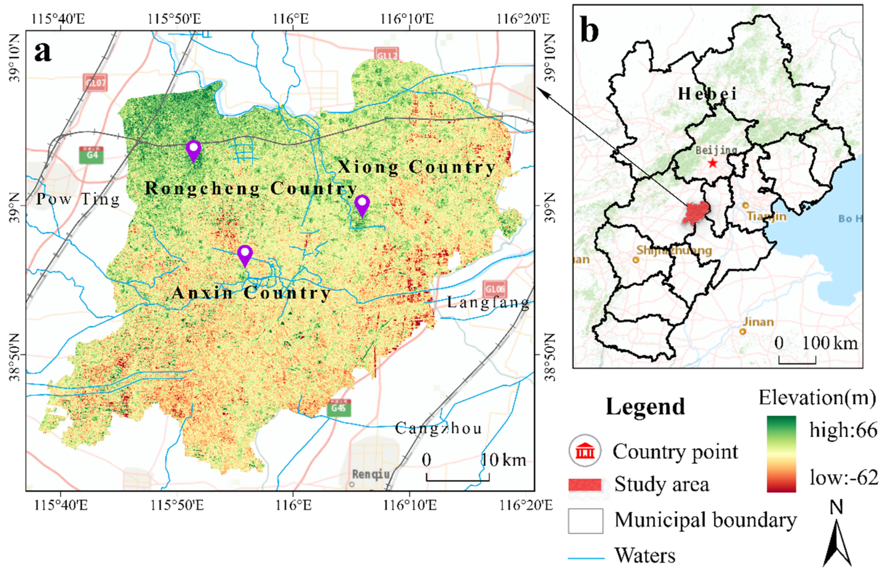
Xiong’an New Area was established in 2017 to relieve the pressure on Beijing’s non-capital function and optimize the urban layouts and spatial structure of the Beijing–Tianjin–Hebei urban agglomeration, which has become a research focus [12,13]. Before the formal designation of Xiong’an New Area, the region included three typical Chinese county towns. Economic development was limited by geographical restrictions and policy support, and the economic growth rate and the GDP were relatively slow and low, respectively. In recent years, improved transportation in this area has led to an increase in the outflow of the population year by year. Although Xiong’an New Area includes Baiyangdian Lake, the largest wetland in the North China Plain which has substantial ecological benefits, its ecological value has diminished year by year owing to its high degree of degradation. On the basis of this development dilemma and the planning objectives, a multi-scenario simulation of land use provided the best opportunity to identify the evolution of agricultural, construction, and ecological land use in the study region, and to guide the formulation of intensive land use policies by the government within the available development space. In addition, the simulation results could be compared with the current regional development trends to provide early warning of problems in land use trends and allow them to be corrected. The selection and application of model drivers offered detailed alternative options for the input conditions and improvement measures needed to develop the study area.
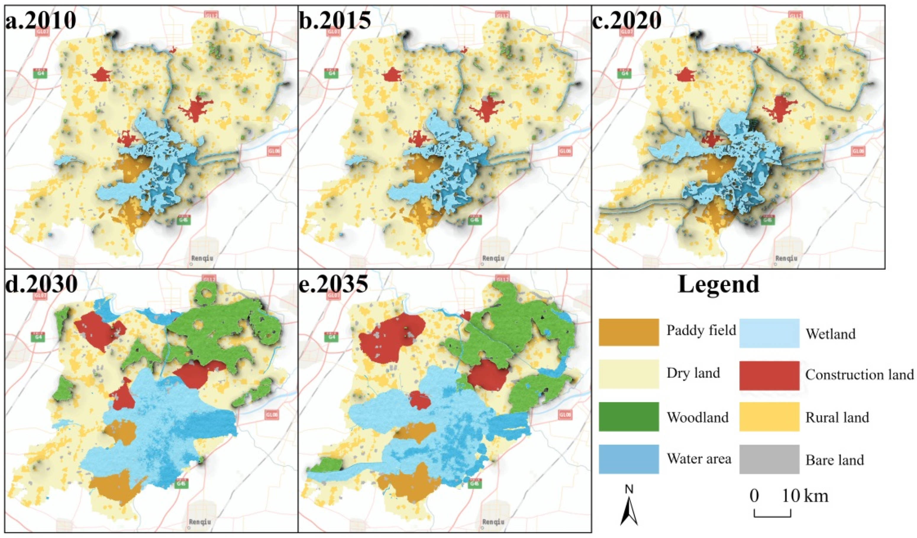
We obtained land use data for Xiong’an New Area in 2010, 2015, and 2020. Sixteen driving factors, including topography, natural factors, socio-economic conditions, and location were used to predict land use change in 2030 and 2035. Xiong’an New Area will be developed into a modern, high-level socialist city by 2035, according to the development goals and requirements for the area. Therefore, 2035 was taken as the time node for the simulation in this study to analyze the agreement between the planning objectives and the simulation results. The land transfer within a certain time range was not a simple linear increase or decrease, but a dynamic process of spatial competition. The model used 2030 as a simulation time node. This was a key step to characterize the dynamic regional land evolution rules and to compare the simulation results predicted for 2035. Therefore, we set the following specific goals. Using the land use data for Xiong’an New Area from 2010 to 2020, four scenarios of land use change (comprehensive evolution, protection of basic farmland, control of construction land, and prioritization of ecological protection) in the study area in 2030 and 2035 were simulated with a Markov–FLUS coupling model and superimposed land conversion conditions. The differences in land use patterns between different scenarios were compared and analyzed. An optimal allocation was proposed in accordance with the research results and the actual situation to optimize the allocation of urban land resources.

2. Literature Review

Much research has focused on optimizing land use change patterns over the past few decades, including theoretical innovation, policy restrictions, early warning of expansion, multi-objective coupling, and the application of big data. These have been combined into an integrated framework. Some studies have used the urbanization process as the background [14], conducting high-level planning research on urban land use change using innovation and ecology as the main driving factors [12]. From another perspective, the reform and diversity of land systems are also important factors affecting land use competition and change [15]. Other studies have analyzed the driving forces of land development rules, mainly focusing on ecology, economy, culture, and distance [16]. To improve on traditional approaches on urban growth phases, researchers have developed the landscape expansion index [17] and green infrastructure factors [18] to analyze the geometric characteristics of land patches and patterns. To meet the practical needs of planners, there has also been also a focus on the mutual feedback mechanism between land management and land transition [19].
The data sources for land use in the base period have a profound impact on the research results. Most studies use remote sensing images as the source of land use data [20], but there can be substantial subjectivity and a lack of consistency in the supervision and classification process [21]. In exploring the problem of urban spatial cohesion, information flow can be used to analyze its changes from a social perspective [22], and the application of the night light index is also an important method for tracking urban sprawl [23]. Some research has focused on a multifractal spectral analysis of construction land in large regions [24], the coupling configuration of different factors, such as the economy and ecology [25], and the bi-fractal structure and evolution of land use morphology [26]. The research on land use change is not limited to urban areas, but also includes river basins [27] and ecologically fragile areas [28].
Along with extensive measures for implementing the construction of an ecological civilization, systematic analysis has been undertaken by various groups, including on the dominant function of land use and spatial cross-analysis. The micro-mechanisms and historical spatial dynamics of urbanization have been explored in depth by incorporating transportation, socio-economic conditions, the ecological pilot rate, and urban affective intensity into the Using the Computable General Equilibrium of Land Use Change (CGELUC) [29]. A special purpose genetic algorithm was used to solve the optimization problem of direct and indirect targets [30]. Some scholars have focused on analyzing the trade-off between ecosystem services and land use. Standard quantification and interaction mechanisms are the main research methods, but they lack a consideration of the spatial factors affecting land allocation [31]. Calculation of the predicted value during land use simulation is a key step for the research results to present the shape.
Common spatial analysis methods and models include the System Dynamic (SD) model [32] and Multi-Agent model [33]. The former is a typical simulation system, which starts from microstructure modeling, and then generates higher-order, nonlinear, and time-varying analysis results on the basis of a feedback loop. This model is suitable for dealing with long-term and periodic problems. The latter can overcome the limitations of traditional macro models and is well suited for a micro simulation of the population location selection process. The Markov Chain model can be used to define the evolution or transfer of land use variables in the time state; that is, it generates a land transfer matrix and pixel values [34]. The time-homogeneity of this model makes the purpose of land transfer more intense. The Computable General Equilibrium of Land Use Change model classifies land into areas that have or do not have a direct economic value for a macro analysis of policy [35]. The Cellular Automata (CA) model is a grid dynamics model in which both the spatial interaction and temporal causality are local [36]. It investigates the whole system through the local effects of simple and discrete cellular units. The basic idea of the CA model corresponds to the feature of “local influence on overall pattern” of land use change. The Conversion of Land Use and its Effects at Sall Region Extent (CLUE–S) model is used to simulate land use change on the basis of empirical and statistical regression methods [
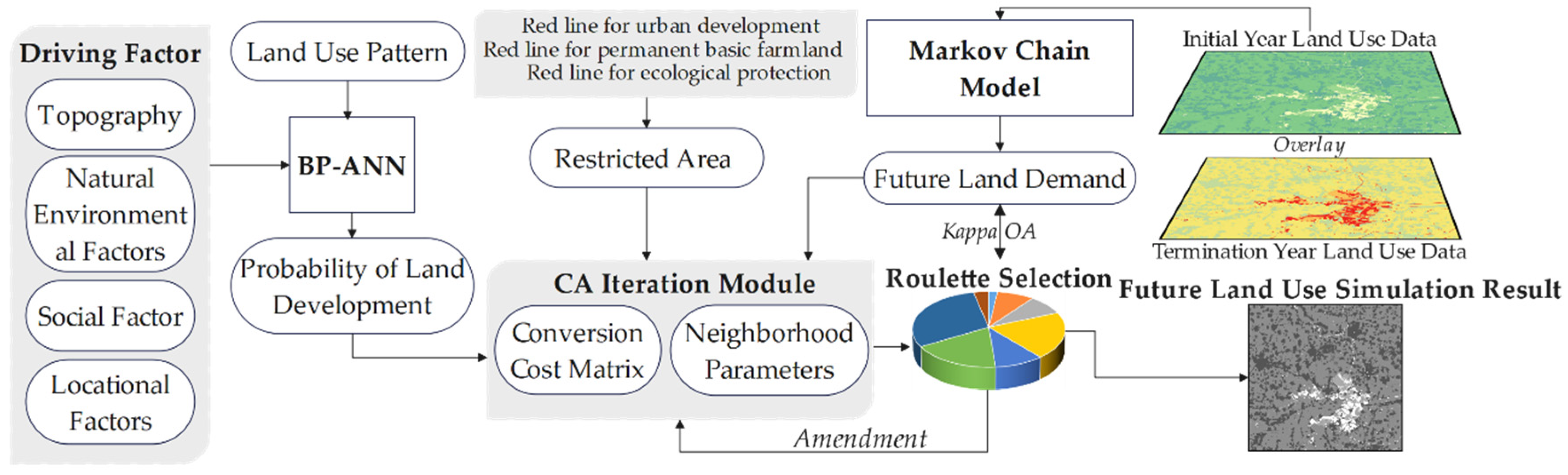
37]. Most scholars use the non-spatial module of changing the strategy preference to define the simulation results, and there are few analyses using the spatial module. The Geographical Simulation and Optimization System–Future Land Use Simulation (GeoSOS–FLUS) model introduces the Artificial Neural Network (ANN) algorithm on the basis of the CA model and SD model, which strengthens the analysis of driving factors of land change research [38]. The CA model has been used in a number of studies because of its advantages for spatio-temporal integration. The FLUS model proposed by Liu Xiaoping, which combines a Back Propagation–Artificial Neural Network (BP–ANN) model, CA model, and other estimation methods, can simulate land use demand under multiple scenarios [39].

3. Material and Methods

3.1. Study Area

Xiong’an New Area is located in central Hebei, 155 km from Shijiazhuang, 105 km from Tianjin, and 55 km from Beijing Daxing Airport (Figure 1. Geographical location of Xiong’an New Area). It includes three counties—Xiongxian, Anxin, and Rongcheng—and 33 townships. There are three rivers—the Daqing, Youyi, and Baigou—and Baiyangdian Lake, which is the largest freshwater wetland in North China. At the end of 2020, the total population was 1.29 million, the per capita GDP was USD 2931, and the urbanization rate was 42.75%.

3.2. Data and Preprocessing

First, according to the research objectives and model requirements, we reclassified the original land use data into eight categories: paddy fields, dry land, woodland, water area, wetland, construction land, rural land, and bare land. Second, we used altitude, slope, and aspect as topographic factors; soil texture and annual average precipitation as natural factors; night light intensity as a social factor; and the road network, railway network, water system, and points of interest (POI, e.g., shopping malls, hotels, schools, banks, and parks) as location factors in the model. The 16 driving factors were normalized using the Euclidean distance and fuzzy membership degree tools of ArcGIS Pro (ESRI, Redlands, CA, USA). The data are detailed in Table 1. Data Information Sources. The current study constructed a multi-factor, multi-scale, multi-scenario, multi-module, and multi-agent integrated Markov–FLUS coupling model [40,41]. According to the document “Planning Outline of Xiong’an New Area, Hebei Province” [42], we established four scenarios: comprehensive evolution, protection of basic farmland, control of construction land, and prioritization of ecological protection. These were used to analyze and simulate land use patterns.

3.3. FLUS Model

To identify the key issues between land use change and the natural environment, Professor Liu Xiaoping from Sun Yat-sen University proposed the FLUS model in 2017 [38]. This model is based on the traditional CA model but includes a Markov model to predict future land change. To calculate the probability of different kinds of land use pixels, multi-band imagery is superimposed to generate a suitability probability file through a BP–ANN module. Then, the land use change simulation is obtained via a roulette competition [43]. Finally, the accuracy is tested using the Kappa coefficient. The investigative framework is shown in Figure 2. A flow chart depicting the analytical process of the research methodology.

3.3.1. Scenario Settings

The comprehensive evolution scenario considered the general evolution rules of land from 2010 to 2020 and included the spatial competition between construction land, prime farmland, and ecological land. Dry land was regarded as the main output source of land conversion, and the probability of other land types being converted to dry land was improved so as to leave sufficient space for the overall regional evolution. The weight of neighborhood land was set according to the proportion of each land class in 2020 to ensure that the final scenario results were in line with the actual effect.
The protection of basic farmland scenario mainly focused on the expansion of paddy fields. Paddy fields have the dual effects of food production and ecological value, which is of great significance for keeping intensive land use, optimizing supply and demand allocation, and improving land use efficiency in Xiong’an New Area. Dry land in the study area was not the main land type in this scenario because it was mostly saline land and had a low grain yield.
The control of construction land scenario took the original construction land in Xiongxian, Rongcheng, and Anxin counties as the origin of expansion, and this gradually approached the initial control area of Xiong’an New Area in the form of clusters according to the planning requirements and its own development characteristics. The expansion of construction land was restricted by the Baiyangdian Lake, the rivers, and the main woodland areas. When construction land was transferred to other land types in this paper, the neighborhood weight was slightly increased and the parameter was set to 1, but the total amount of construction land was limited to less than 30% in the scenario simulation.
In the prioritization of ecological protection scenario, paddy fields, woodland, water area, and wetland were taken as the main expansion land types, and the transformation matrix of the land in the scenario was allocated comprehensively (Table 2. Simulation Cost Matrix under the Multi-Scenario Space Priority). The transfer cost of blue–green space was higher than that of other land types. Wetlands within the main protection area had the same transfer cost as water with less distribution, and the cost was higher than that of woodland and paddy fields. On the basis of past research experience and the human and natural characteristics of the study area [44,45], the neighborhood weight relationship of wetland = woodland = construction land > rural land > water area > dry land > paddy fields > bare land was set according to the resistance relationship per unit area of land. The neighborhood weight of ecological land was slightly increased owing to the Xiong’an New Area Ecological Environment Protection Plan and Baiyangdian wetland restoration work.

3.3.2. Probability of Land Development

BP–ANN is a multi-layer feed forward neural network, including an input layer, one or more hidden layers, and an output layer [38]. It was divided into two main stages, training, and evaluation:
τ ( p ,   k ,   t ) = j w j ,   k × sigmoid ( net j ( p ,   t ) ) = j w j ,   k × 1 1 + e net j ( p ,   t )
where τ ( p ,   k ,   t ) is the suitability probability of k land type at time t and grid p ; w j ,   k is the weight between the hidden layer and the output layer; sigmoid   (   ) is the excitation function from the hidden layer to the output layer; net j   ( p ,   t ) is the signal value received by the j -th hidden layer grid p at time t . The sum of the suitability probabilities of each land type output in BP–ANN is always 1, namely:
j τ ( p ,   k ,   t ) = 1

3.3.3. Conversion Cost Matrix and Neighborhood Parameters

The land conversion cost matrix indicated the ease of transforming a current land type into a target type. The conversion probability was subject to neighborhood density, a conversion weight, spatial resolution, land type competition, and an adaptive inertia coefficient. The adaptive inertia coefficient was determined by the gap between the actual land use quantity and the target demand quantity, which was adapted in the iteration to approach the target trend gradually [44]:
Inertia k t = { Inertia k t 1 | D k t 2 | | D k t 1 | Inertia k t 1 × D k t 2 D k t 1 0 > D k t 2 > D k t 1 Inertia k t 1 × D k t 1 D k t 2 D k t 1 > D k t 2 > 0
where Inertia k t is the inertia coefficient of k land at the t -th iteration time; D k t 1 , D k t 2 is the difference between the practical grids and the target grids at the t 1 , t 2 time.
Through the above steps, we obtained the probability TProb p ,   k t that grid p could be converted into k land at t time. Each land type could be allocated to the grid through the CA iteration, and the expression was [39]:
TProb p ,   k t = τ ( p ,   k ,   t ) × Ω p ,   k t × Inertia k t × ( 1 sc c k )
Ω p ,   k t = N × N con ( c p t 1 = k ) N × N 1 × w k
where sc c k is the cost of converting the original land use type c into type k , 1 sc c k represents the difficulty of conversion; Ω p ,   k t denotes Moore density; N × N con   ( c p t 1 = k ) is the quantity of grids of k land at the end of t 1 time on the N × N Moore window; w k is the weight of k land types.

3.4. Markov Model

The Markov Chain stochastic model can simulate and predict the development trend of land through the transition probability matrix, on the basis of the occurrence probability of multi-period land types [34]. The transition probability of n period p ij n and the final percentage matrix A ( n ) were expressed as:
p i   j n = k = 0 m 1 p k   j n 1 = k = 0 m 1 p i   k n 1 × p k   j
A ( n ) = A ( n 1 ) × p i   j 1 = A ( 0 ) × p i   j n
where m is the row number and column number of the transition probability matrix; and A ( 0 ) is the initial land area percentage matrix.
First, BP–ANN was used to calculate the probability of land conversion in 2010. Then, on the basis of the land use data in 2010 and combined with the land probability calculation results, the Markov Chain model was introduced to predict the land use in 2030 and 2035, respectively. The land use scales of 2015 and 2020 were extracted from the above predicted results and spatially expressed by CA. Finally, the actual land use in 2015 and 2020 was compared with the predicted results to obtain the accuracy of the Markov Chain model in predicting future land use. The accuracy test results also represented the accuracy of land use in 2030 and 2035 that was predicted using the land use data in 2020, following the same process as indicated previously. The number of pixels of each land use type is shown in Table 3. Present and Future Number of Pixels in Different Land Use Types.

3.5. Kappa and Overall Accuracy Precision Inspection

The Kappa coefficient is a scale that represents the proportion of categorization to the reduction in errors produced by completely random categorization. The calculation of kappa coefficients is based on a confusion matrix and is between −1 and 1, usually greater than 0. However, in the classification problem of this study, the number of samples in each category was not balanced. Without adjustments on such imbalanced data sets, models can easily favor large categories over small ones. Therefore, the kappa accuracy can better express the quantitative accuracy and spatial distribution accuracy of the predicted results. The expression was [44]:
K = ( P a P b ) / ( 1 P b )
where P a represents the same proportion of the simulation results, and P b represents the correct proportion of the simulation results of targets chosen at random.
Overall accuracy is the ratio between what the model predicted correctly on all test sets and the overall number. The model shows a high accuracy with Kappa ≤ 0.75 and an overall accuracy (OA) < 1, a moderate accuracy with Kappa ≤ 0.5 and an OA < 0.75, and a poor accuracy with Kappa ≤ 0 and OA < 0.5.

4. Results

The quantity of each land type in Xiong’an New Area in 2030 and 2035 that was predicted by the Markov–FLUS coupling model in the four scenarios—comprehensive evolution, protection of basic farmland, control of construction land, and prioritization of ecological protection—is shown in Table 4. Land Area and Proportion in the four Scenario Simulations. More detail about the rate and range of change in land use under different restrictions from 2010 to 2035 is shown in Table 5. Annual Degree and Amplitude of Change in Land Use from 2010 to 2035 (%). The two-phase simulation Kappa was 0.9675 and 0.7892, while the OA was 0.9827 and 0.8805. The simulated prediction had a high level of accuracy.
In the simulations of the four scenarios, the annual dynamics and amplitude changes in the land use in the comprehensive evolution scenario were less extreme compared with the other three scenarios. In the protection of basic farmland scenario, the increase in the area of paddy fields far exceeded that of other scenarios in the same period, with an increase of 228.42% from 2010 to 2035. The final area of paddy fields accounted for 9.96% of the total land area. In the control of construction land scenario, the expansion of construction land into blue–green space (paddy fields, woodland, water area, wetland) was substantial. In 2035, the proportion of blue–green space was the lowest in the same period. In the prioritization of ecological protection scenario, the blue–green space accounted for 52.40% in 2035, with an area of 93.59 km2. The simulations showed that the different land uses maintained a balanced state in multiple scenarios and coordinated development of the production–living–ecological space continued, which improved the sustainability of land use.

4.1. Comprehensive Evolution Scenario

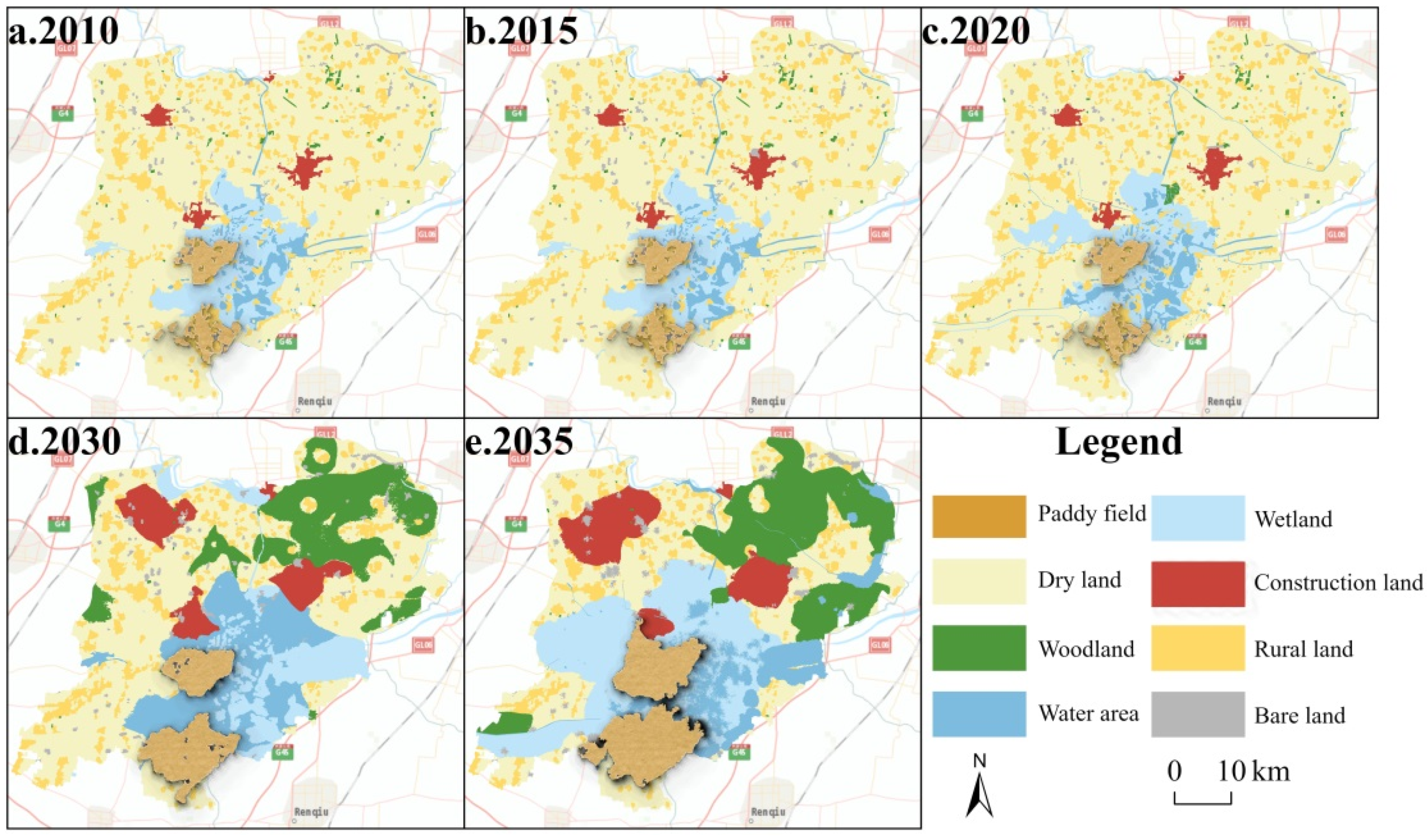
The comprehensive evolution scenario simulation showed that the spatial pattern of the land in this area maintained a balance of blue–green land uses (Figure 3. Comparison of land use over time in the comprehensive evolution scenario). By 2035, a planned urban–rural spatial structure with comprehensive functions had formed, along with a clustered urban spatial pattern integrated with water areas.
Dry land showed a significant decrease, with an annual change rate of −2.12% (Table 4. Land Area and Proportion in the four Scenario Simulations). From 2010 to 2035, there was a steady increase in paddy fields, mostly converted from dry land. Construction land steadily expanded from 2010 to 2035, with an annual change rate of 14.6%, which was second only to woodland. In addition to expanding the urban extent in the original counties and townships, new construction land mainly extended to the northwest of the Baiyangdian Lake. In 2035, wetlands accounted for 20.1% (Table 6. Land Use Area and Percentage in the Comprehensive Evolution Scenario), and the core area of lake wetlands occurred in the southwest of the study area. In Northeast China, the area of woodland patches increased significantly. In the study area, from 2010 to 2035, the annual change rate of woodland reached 124.01%, and the coverage increased from 0.54% to 17.9%. In 2035, the main water area reached 175 km2, forming a landscape-level corridor and node system.
In the comprehensive evolution scenario, the area growth of paddy fields was significantly lower than that of other scenarios. In 2035, the area of basic farmland in this scenario was 60.44 km2, only just higher than 60.11 km2 in the scenario of control of construction land in the same period. In this scenario, the construction land expansion results were substantial, and the construction land area in 2035 was 150.13 km2, accounting for 8.41%, which was higher than that in the protection of basic farmland scenario and prioritization of ecological protection scenario in the same period. The proportion of blue–green space in the comprehensive evolution scenario was low, and the area proportion in 2030 and 2035 was 43.4% and 51.35%, respectively, which was lower than that in the prioritization of ecological protection scenario.

4.2. Protection of Basic Farmland Scenario

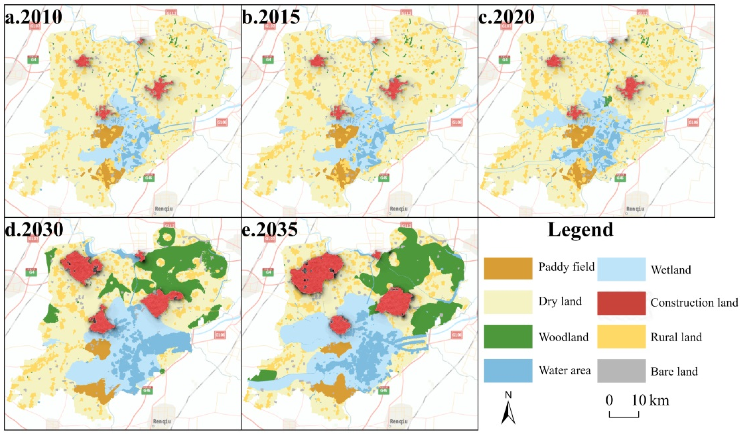
In the protection of basic farmland scenario, on the basis of land use change in 2010 to 2020 and considering the multiple requirements for basic farmland protection, the model decreased the conversion ratio of other land types to paddy fields, with the highest transfer matrix rank and an expanded land suitability probability. Xiong’an New Area’s plan requires 18% of cultivated land and 10% of permanent basic farmland.
The protection of basic farmland scenario simulation showed that the area of paddy fields increased from 54.18 km2 to 53.68 km2 from 2010 to 2020, and the growth trend accelerated from 2010 to 2035 (Table 4. Land Area and Proportion in the four Scenario Simulations), with an annual change rate of 8.79%. By 2035, the proportion of paddy fields was 9.96%, with an area of 178 km2 (Table 7. Land Use Area and Percentage in the Protection of Basic Farmland Scenario). Because the paddy fields were adjacent to key ecological areas, there was some cross-integration in the expansion process of the two land use types, according to the neighborhood impact theory (Figure 4. Comparison of land use differences in the protection of basic farmland scenario). The overall weight of farmland transfer was greater than that of wetlands, resulting in the conversion of some wetlands to paddy fields southwest of the Baiyangdian Lake.
In the protection of basic farmland scenario, the annual dynamic and amplitude change in the paddy fields from 2010 to 2035 were much higher than those of the other three scenarios, amounting to 8.79% and 228.42% (Table 5. Annual Degree and Amplitude of Change in Land Use from 2010 to 2035 (%)), respectively, which were the maximum year-on-year values. The development of woodland in this scenario was more limited, and the 2010–2035 annual dynamic was 120.01%, which was lower than that in the other three scenarios. However, it had a positive effect on the overall blue–green space area. In 2035, the blue–green space occupied 57.36% and the area was 1024.63 km2, which was the maximum in that period.

4.3. Control of Construction Land Scenario

In the control of construction land scenario, the transfer probability for construction land was greater than that of other land types. In line with the planning requirements, the predicted demand for construction land was limited to 30%, with an area of approximately 530 km2. The target threshold for rural land areas was limited to 50 km2, accounting for 3%, as well as a proportion of bare land within the control range.
The simulation results for the control of construction land scenario showed that the proportion of construction land in 2030 and 2035 was 6.52% and 8.78%, respectively (Table 8. Land Use Area and Percentage for the Control of Construction Land Scenario). The area was 116.37 km2 and 156.79 km2, respectively, and the change rate from 2010 to 2035 was 15.47% (Table 4. Land Area and Proportion in the four Scenario Simulations). The rural land that used to be concentrated in the northwest decreased by 43.61% from 2010 to 2035 (Figure 5. Comparison of land use differences in the control of construction land scenario), and the occupied area approached the target value of 50 km2. In the process of change, the stable proportion of bare land was 2%, and the area was 35 km2.
Compared with the other scenarios, the proportion of construction land increased significantly. It was approximately 0.5% higher than that of the other scenarios, and a small amount of ecological land was encroached upon. In 2035, the proportion of blue–green space was 51.13%, with an area of 913 km2, which was the lowest at the same date among all scenarios. The water area and wetland in the control of construction land scenario were not affected in the expansion process, and the annual dynamic and amplitude changes from 2010 to 2035 were the same as those in the other three scenarios.

4.4. Prioritization of Ecological Protection Scenario

In the prioritization of ecological protection scenario, the target threshold for woodland coverage rate was set to 40%. Full play was given to the ecological regulation function of paddy fields and their transfer cost probability could be expanded within a certain range.
The simulation results for the prioritization of ecological protection scenario showed that by 2035, Xiong’an New Area will have a blue–green spatial pattern with large woodland patches in the northeast and Baiyangdian Lake wetland and the water system will be connected in the southwest (Figure 6. Comparison of land use differences in the prioritization of ecological protection scenario). The wetland area increased significantly. In 2035, wetlands accounted for 20.15% (360 km2) (Table 9. Land Use Area and Percentage in the Prioritization of Ecological Protection Scenario), with an overall increase of 137.58% (Table 4. Land Area and Proportion in the four Scenario Simulations). The water area increased from 63.16 km2 in 2010 to 175.86 km2 in 2035. In 2035, woodland accounted for 17.72%, or 316.42 km2, and the change rate from 2010 to 2035 was up to 122.24%, which was the highest in the same period among all scenarios.
In the prioritization of ecological protection scenario, blue–green space accounted for 52.4%, which was higher than two of the other scenarios, but still lower than that in the protection of basic farmland scenario. It can be seen that the environmental development of Xiong’an New Area should not only consider simple ecological factors, but land uses should complement each other with ecological and production space. In 2035, the area of construction land will be 144.8 km2, the lowest in the same period. The area of woodland expansion in this scenario was smaller than that in the comprehensive evolution scenario, and the annual dynamic was 122.24%.

5. Discussion

5.1. Study Compared

Compared with other articles on the same topic, this study has some unique and innovative characteristics in terms of the selection of the study area, the setting of scenario types, and the purposes of the simulation. We chose Xiong’an New Area as the research area because before its establishment by the government, this area was not on the path to becoming a high-quality city. Most previous studies (Table 10. Land Use Area and Percentage in the Protection of Basic Farmland Scenario) have focused only on study areas with good infrastructure and significant expansion. Therefore, the problem addressed in this paper was to simulate and optimize the future land pattern in the absence of a mature development foundation and clear land development trends in the region.
In setting the scenarios, we concentrated on independent land expansion scenarios of production, living, and ecology, and added a comprehensive evolution scenario. This method can consider the competition between different land types and present the future vision of the study area that best conforms to the regulation of land evolution. When the land types included in the four scenarios were initially classified, the cross-attribution method was adopted for the land types with multi-layer values. For example, paddy fields existed in both basic farmland and blue–green space. This division is consistent with the actual situation of land use values and improves the contribution of land values.
Compared with similar studies [48], we used a Markov Chain model to predict future land use. Compared with the SD model, we paid more attention to the change of land quantity in the future prediction mechanism, rather than the rational change of driving factors using mathematical statistics in linear analysis. This difference will lead to differences in land demand in the study, and the final simulation results will also be different. Second, among the four scenario parameter settings, the “Production–Life–Ecology” space was used in our study to distinguish the results, rather than as the setting condition of a scenario. Instead of using population, GDP, and scientific and technological innovation as scenario parameters for analysis, we adopted the key development of the dominant land category in the scenario. For example, we set the transfer probability and neighborhood weight of woodland in the ecological protection scenario far higher than other scenarios. There were also fundamental differences in the division of situations. Finally, the research purpose of this paper was the overall land use pattern of Xiong’an New Area, and the analysis showed how the integrated development of various spaces could be achieved for land use consolidation or optimal development. Ecological environmental factors were an important part of the research and analysis but were not the main research purpose of this paper.

5.2. Simulation Results

With reference to the previous spatial analysis of land use in the same study area [48,49], the simulation results of the Markov–FLUS coupling model integrated multiple impacts, such as natural conditions, social policies, human activities, and ecological protection. In the future plan, Xiong’an New Area is dominated by blue–green space. In the final simulation, the area of blue–green land reached 51.35%, accounting for an increase of 36.81%. The model accurately calculated the demands of land use change for the ecological environment and met the planning vision to some extent. The simulation and prediction results are related to the land development and protection pattern and ecosystem service value of Xiong’an New Area. The expansion of construction land based on the three counties and districts formed a good connection with the development of urban clusters. In previous research on land use change in Xiong’an New Area, the simulation results seldom included production and living spaces. The current study included a detailed systematic analysis of the main development land types for multiple scenarios. For example, to consider the impact of the conflict between the expansion of construction land and the expansion of adjacent wetlands [51], the number of iterations was increased to 300, and the coordinated coupling of the three living spaces was realized through a multi-change simulation process. This addresses the limitation of single-goal development and is more in line with the practical significance and spatial value of Xiong’an New Area [50,52].

5.3. Application of Research Results

First, the research results included most of the land considered in the planning of Xiong’an New Area, covering an area of 1786 km2. The blue–green space was in a state of sustained and rapid growth, but it was well below the 70% proportion required by the plan. Therefore, relying solely on ecological restoration and management measures, such as afforestation, returning farmland to lakes, and dredging water systems in the region is unlikely to achieve the planning objectives. Cross-regional and high-intensity multi-source water replenishment measures are needed, such as diverting the Yellow River into Hebei to replenish lakes and supply upstream reservoirs. The detailed simulation results at a resolution of 30 m can assist with a precise delineation of the urban development boundary, the permanent basic farmland protection red line, and the ecological protection red line in Xiong’an New Area [51]. The negative effects of land development can be avoided through an early warning of conflicts between adjacent spaces, planning control, and prevention [46,53]. Second, among the simulation results from the four scenarios, the comprehensive evolution scenario can provide a background blueprint conforming to the planned development direction. The simulations for the protection of basic farmland and the control of construction land can provide support for building a scientific urban and rural spatial structure by visualizing the future development of the anthropogenic environment from the perspective of production and living spaces [54]. The results from the ecological prioritization scenario, coupled with other scenarios, not only provide a global perspective for the ecological restoration and management of Baiyangdian Lake but they also provide options for protecting ecological sources, constructing ecological corridors, and creating new blue–green spaces [12,55]. Finally, Xiong’an New Area needs to undertake the transfer of Beijing’s non-capital functions. The research results of this paper demonstrate how the spatial allocation and optimization of the land use pattern can be used to create an innovative geographical space [47,56].

5.4. Limitations and Prospects

The Markov–FLUS coupling model was used to simulate the land use and spatial pattern in multiple scenarios, considering human and natural factors. However, owing to the complexity of the research objective, the driving factors used in the model were selected through theoretical analysis and references to previous studies, which had a degree of subjectivity. If a linear analysis of driving factors was carried out, the influence of each driving factor on the simulation could be analyzed, and the driving factors that met the characteristics of the study could selected for subsequent research. This would improve the simulation results. The impact of policy on land use change in the FLUS model can only be expressed in the setting of parameters, which has its own limitations. The policy index system can be transformed into geospatial elements and coupled with the simulation model, which will be a breakthrough in future research [57]. In addition, the land use classification in this paper was mainly based on the study of suitability, and no evaluation system was constructed to calculate the division of land types. The land use classification had insufficient detail and there was a lack of further systematic division of the internal green space of urban areas [52,58]. Subsequently, more detailed scale simulation analysis and comparisons could be carried out for different regions to solve the lack of control standards, find a more reasonable evaluation system for land expansion indicators, make the land use pattern results closer to reality, and better simulate the process of land use change and development.

6. Conclusions

In this paper, the analysis of dynamic change in land use and the optimization application of multi-scenario simulation results achieved excellent results. The probabilistic calculation of land suitability constructed by social, economic, demographic, and natural factors can provide scientific advice on the maximum probability of various land use changes for cities with minor past land changes or for newly established cities. The detail contained in the classification system of land use limits whether there is convergence or exclusion of different spatial distribution boundaries. Research proved that the simulation result was able to realize the optimal planning intervention measures of sustainable development of an inland city, because it could predict areas of rapid expansion (especially in large or emerging cities) and tailor those on a regional basis toward the specified scope of sustainable land planning to control urban sprawl and urban growth. The four scenarios could all provide suggestions for corresponding spatial patterns.
(i)
According to the comprehensive evolution scenario, the wetland continued to expand in the southwest of the region, which did not meet the construction needs of the ecological corridor in the middle and north of the region. In Anxin County, the construction land for human settlements and industry should be controlled in a timely fashion, and sufficient development space should be reserved for wetland or other ecological land.
(ii)
Basic farmland will be eroded by dry land and infrastructure construction. Relevant departments should strengthen the construction of high-quality farmland to ensure that the total amount of permanent basic farmland does not decrease, the use of permanent basic farmland does not change, and the quality of permanent basic farmland is improved.
(iii)
The peripheral cluster mode of construction land will be basically completed in 2035, but the distribution pattern of bare land is chaotic. It would be a reasonable governance measure to strictly control the boundaries of urban development and the size of the urban population, and to leave strategic space blank for national major development strategies and sustainable urban development.
(iv)
The scale of blue–green space improved greatly, but there was still a gap with the planning target threshold. As a community that sustains life, the wetland and woodland should be protected and restored in a unified manner to ensure the integrity of the new ecological system.

Author Contributions

Conceptualization, J.H. and Z.S.; methodology and software, J.H.; validation, H.X.; formal analysis, X.C.; data curation, visualization, and writing—original draft preparation, J.H. and W.Z.; writing—review and editing, J.H. and Z.S. All authors have read and agreed to the published version of the manuscript.

Funding

This research was funded by the National Key R&D Program of China (2021YFE0106700).

Institutional Review Board Statement

Not applicable.

Informed Consent Statement

Not applicable.

Data Availability Statement

The data presented in this study are available on request from the corresponding author.

Acknowledgments

We thank Leonie Seabrook, for editing the English text of a draft of this manuscript.

Conflicts of Interest

The authors declare no conflict of interest.

References

  1. Liu, J.Y.; Zhang, Z.X.; Zhang, S.W.; Yan, C.Z.; Wu, S.X.; Li, R.D.; Kuang, W.H.; Shi, W.J.; Huang, L.; Ning, J.; et al. Innovation and development of remote sensing-based land use change studies based on Shupeng Chen’s academic thoughts. J. Geo-Inf. Sci. 2020, 22, 680–687. [Google Scholar]
  2. Lambin, E.F.; Geist, H.J. Land-Use and Land-Cover Change: Local Processes and Global Impacts; Springer: New York, NY, USA, 2006; pp. 5–22. [Google Scholar]
  3. Collins, M.; Steiner, F.; Rushman, M. Land-Use Suitability Analysis in the United States: Historical Development and Promising Technological Achievements. Environ. Manag. 2001, 28, 611–621. [Google Scholar] [CrossRef] [PubMed]
  4. Frederick, S.; Laurel, M.S.; Jill, C. Land suitability analysis for the upper Gila River watershed. Landsc. Urban Plan. 2000, 50, 199–214. [Google Scholar]
  5. Liu, J.Y.; Zhang, Z.X.; Xu, X.L.; Kuang, W.H.; Zhou, W.C.; Zhang, S.W.; Li, R.D.; Yan, C.Z.; Yu, D.S.; Wu, S.X.; et al. Spatial patterns and driving forces of land use change in China in the early 21st century. J. Geogr. Sci. 2009, 64, 1411–1420. [Google Scholar] [CrossRef]
  6. Lu, D.D. The Development of economic geography and its function on strategy consultation. Econ. Geogr. 2011, 31, 529–535. [Google Scholar]
  7. Fan, J.; Zhou, K.; Sun, W.; Chen, D. Scientific values and research innovations of Human-economic Geography in construction of ecological civilization. Prog. Geogr. 2013, 32, 147–160. [Google Scholar]
  8. Zhang, C.; Wang, P.; Xiong, P.; Li, C.; Quan, B. Spatial Pattern Simulation of Land Use Based on FLUS Model under Ecological Protection: A Case Study of Hengyang City. Sustainability 2021, 13, 10458. [Google Scholar] [CrossRef]
  9. Huang, J.C.; Lin, H.X.; Qi, X.X. A literature review on optimization of spatial development pattern based on ecological–production–living space. Prog. Geogr. 2017, 36, 378–391. [Google Scholar]
  10. Fan, J.; Zhao, Y.N. China’s regional development pattern oriented toward modernization: The scientific connotation and strategic priorities. Econ. Geogr. 2021, 41, 1–9. [Google Scholar]
  11. Domingo, D.; Palka, G.; Hersperger, A.M. Effect of zoning plans on urban land-use change: A multi-scenario simulation for supporting sustainable urban growth. Sustain. Cities Soc. 2021, 69, 102833. [Google Scholar] [CrossRef]
  12. Ge, Q.S.; Dong, X.F.; Mao, Q.Z.; Zhang, W.Z.; Du, L.J.; Zhang, W.; He, C.Y.; Wu, D.T.; Lv, L.C.; Chen, M.X.; et al. How to build Xiong’an New Area into an ecological and innovation city? Geogr. Res. 2018, 37, 849–869. [Google Scholar]
  13. Kuang, W.H.; Yang, T.R.; Yan, F.Q. Regional urban land-cover characteristics and ecological regulation during the construction of Xiong’an New District, Hebei Province, China. J. Geogr. Sci. 2017, 72, 947–959. [Google Scholar]
  14. Gu, C.L.; Wu, L.Y.; Ian, C. Progress in research on Chinese urbanization. Front. Archit. Res. 2012, 2, 101–149. [Google Scholar]
  15. Shi, C.; Tang, B.S. Institutional change and diversity in the transfer of land development rights in China: The case of Chengdu. Urban Stud. 2020, 57, 473–489. [Google Scholar] [CrossRef]
  16. Zhao, D.L.; Du, M.; Yang, J.Y.; Li, P.S.; He, S.S.; Zhu, D.H. Simulation and forecast study of land use change based on CA–Markov model. Trans. Chin. Soc. Agric. Mach. 2016, 47, 278–285. [Google Scholar]
  17. Liu, X.P.; Li, X.; Chen, Y.M.; Qin, Y.; Li, S.Y.; Chen, M.H. Landscape expansion index and its applications to quantitative analysis of urban expansion. J. Geogr. Sci. 2009, 64, 1430–1438. [Google Scholar]
  18. Hu, T.H.; Chang, J.; Liu, X.X.; Feng, S.S. Integrated methods for determining restoration priorities of coal mining subsidence areas based on green infrastructure—A case study in the Xuzhou urban area, of China. Ecol. Indic. 2018, 94, 164–174. [Google Scholar] [CrossRef]
  19. Long, H.L.; Qu, Y. Land use transition and land management. Geogr. Res. 2015, 34, 1607–1618. [Google Scholar]
  20. Chen, Z.; Huang, M.; Zhu, D.; Altan, O. Integrating remote sensing and a Markov–FLUS model to simulate future land use changes in Hokkaido, Japan. Remote Sens. 2021, 13, 2621. [Google Scholar] [CrossRef]
  21. Yao, Y.; Li, X.; Liu, X.P.; Liu, P.H.; Liang, Z.T.; Zhang, J.B.; Mai, K. Sensing spatial distribution of urban land use by integrating points-of-interest and Google Word2Vec model. Int. J. Geogr. Inf. Sci. 2016, 31, 825–848. [Google Scholar] [CrossRef]
  22. Lin, Q.; Xiang, M.Y.; Zhang, L.; Yao, J.; Wei, C.; Ye, S.; Shao, H. Research on Urban Spatial Connection and Network Structure of Urban Agglomeration in Yangtze River Delta—Based on the Perspective of Information Flow. Int. J. Environ. Res. Public Health 2021, 18, 10288. [Google Scholar] [CrossRef]
  23. Paul, C.S. A scale-adjusted measure of “Urban Sprawl” using nighttime satellite imagery. Remote Sens. Environ. 2003, 86, 353–369. [Google Scholar]
  24. Huang, L.S.; Chen, Y.G.; Li, S.C. Multifractal spectral analysis of land use structure of the Beijing–Tianjin–Hebei urban system. Prog. Geogr. 2019, 38, 50–64. [Google Scholar]
  25. Ma, B.Y.; Huang, J.; Li, S.C. Optimal allocation of land use types in the Beijing–Tianjin–Hebei urban agglomeration based on ecological and economic benefits trade-offs. Prog. Geogr. 2019, 38, 50–64. [Google Scholar]
  26. Zhao, J.T.; Chen, Y.G.; Li, S.C. Bi-fractal structure and evolution of the Beijing–Tianjin–Hebei region urban land-use patterns. Prog. Geogr. 2019, 38, 77–87. [Google Scholar]
  27. Zhu, W.; Zhang, J.; Cui, Y.; Zhu, L. Ecosystem carbon storage under different scenarios of land use change in Qihe catchment, China. J. Geogr. Sci. 2020, 30, 1507–1522. [Google Scholar] [CrossRef]
  28. Feng, D.; Bao, W.; Fu, M.; Zhang, M.; Sun, Y. Current and Future Land Use Characters of a National Central City in Eco-Fragile Region—A Case Study in Xi’an City Based on FLUS Model. Land 2021, 10, 286. [Google Scholar] [CrossRef]
  29. Huang, J.C.; Lin, H.X. Spatial evolution analysis and multi-scenarios simulation of Beijing–Tianjin–Hebei urban agglomeration. Geogr. Res. 2017, 36, 506–517. [Google Scholar]
  30. Theodor, J.S.; Ron, J. A multi-objective GIS-based land use planning algorithm. Comput. Environ. Urban Syst. 2014, 46, 25–34. [Google Scholar]
  31. Andrea, K.; Anna, F.C.; Martin, V. A review of multi-criteria optimization techniques for agricultural land use allocation. Environ. Modell. Soft. 2018, 105, 79–93. [Google Scholar]
  32. Charles, P.N.; Holger, R.M.; Aaron, C.Z.; Jeffrey, P.N.; Hedwig van, D. Multi-objective optimization framework for calibration of Cellular Automata land-use models. Environ. Modell. Soft. 2018, 100, 175–200. [Google Scholar]
  33. Li, S.Y.; Li, X.; Liu, X.P.; Wu, Z.F.; Ai, B.; Chen, M.H.; Li, H.B.; Liu, M.W. Multi-scenario simulations on the interactions of jobs-housing based on agent-based model. J. Geogr. Sci. 2013, 68, 1389–1400. [Google Scholar]
  34. Wang, M.; Cai, L.Y.; Xu, H.; Zhao, S.L. Predicting land use changes in northern China using logistic regression, cellular automata, and a Markov model. Arab. J. Geosci. 2019, 12, 4291–4301. [Google Scholar] [CrossRef]
  35. Jin, G.; Chen, K.; Wang, P.; Guo, B.S.; Dong, Y.; Yang, J. Trade-offs in land-use competition and sustainable land development in the North China Plain. Technol. Forecast. Soc. Chang. 2019, 141, 36–46. [Google Scholar] [CrossRef]
  36. Li, X.; Chen, Y.M.; Liu, X.P.; Xu, X.C.; Chen, G.L. Experiences and issues of using cellular automata for assisting urban and regional planning in China. Int. J. Geogr. Inf. Sci. 2017, 31, 1606–1629. [Google Scholar] [CrossRef]
  37. Zhang, J.; Zhu, W.B.; Wu, S.Y.; Li, S.C. Simulation of temporal and special land use changes in Jing–Jin–Ji urban agglomeration using CLUE–S model. Acta Sci. Nat. Univ. 2018, 54, 115–124. [Google Scholar]
  38. Cao, S.; Jin, X.B.; Yang, X.H.; Sun, R.; Liu, J.; Han, B.; Xu, W.Y.; Zhou, Y.K. Coupled MOP and GeoSOS–FLUS models research on optimization of land use structure and layout in Jintan district. J. Nat. Resour. 2019, 34, 1171–1185. [Google Scholar] [CrossRef]
  39. Liu, X.P.; Liang, X.; Li, X.; Xu, X.C.; Ou, J.P.; Chen, Y.M.; Li, S.Y.; Wang, S.J.; Pei, F.S. A future land use simulation model (FLUS) for simulating multiple land use scenarios by coupling human and natural effects. Landsc. Urban Plan. 2017, 168, 94–116. [Google Scholar] [CrossRef]
  40. Fang, C.L.; Zhou, C.H.; Gu, C.L.; Chen, L.D.; Li, S.C. Theoretical analysis of interactive coupled effects between urbanization and eco-environment in mega-urban agglomerations. J. Geogr. Sci. 2016, 71, 531–550. [Google Scholar] [CrossRef]
  41. Zhang, J.; Zhu, W.; Zhu, L.; Cui, Y.; He, S.; Ren, H. Topographical relief characteristics and its impact on population and economy: A case study of the mountainous area in western Henan, China. J. Geogr. Sci. 2019, 29, 598–612. [Google Scholar] [CrossRef] [Green Version]
  42. Xiao, X.R. Research on the Development Concept of Xiong’an New Area Based on Beijing–Tianjin–Hebei Coordinated Development. In Proceedings of the 5th International Conference on Education Technology, Management and Humanities Science (ETMHS 2019), Jawa Timur, Indonesia, 3–5 October 2019. [Google Scholar]
  43. Zhao, L.F.; Liu, X.P.; Liu, P.H.; Chen, G.Z.; He, J.L. Urban expansion simulation and early warning based on geospatial partition and FLUS model. J. Geo-Inf. Sci. 2020, 22, 517–530. [Google Scholar]
  44. Li, G.Z. Land Use Change and Simulation in Shenzhen Based on FLUS Model; Wuhan University: Wuhan, China, 2018. [Google Scholar]
  45. Zhang, X.H.; Xu, W.B.; Zhang, B.A. Pre-evaluation of the role of Xiong’an new district in the low carbon synergy development of Beijing–Tianjin–Hebei urban agglomeration. Econ. Geogr. 2020, 40, 16–23. [Google Scholar]
  46. Zhang, J.D.; Mei, Z.X.; Lu, J.H.; Chen, J.Z. Simulating multiple land use scenarios based on the FLUS model considering spatial autocorrelation. J. Geo-Inf. Sci. 2020, 22, 531–542. [Google Scholar] [CrossRef]
  47. Ou yang, X.; He, Q.Y.; Zhu, X. Simulation of impacts of urban agglomeration land use change on ecosystem services value under Multi-Scenarios: Case study in Changsha–Zhuzhou–Xiangtan urban agglomeration. Econ. Geogr. 2020, 40, 93–102. [Google Scholar]
  48. Wang, Z.; Cao, J.; Zhu, C.; Yang, H. Assessing and Predicting the Impact of Multi-Scenario Land Use Changes on the Ecosystem Service Value: A Case Study in the Upstream of Xiong’an New Area, China. Sustainability 2021, 13, 704. [Google Scholar] [CrossRef]
  49. Xu, H.Q.; Shi, T.T.; Wang, M.Y.; Lin, Z.L. Land cover changes in the Xiong’an New Area and a prediction of ecological response to forthcoming regional planning. Acta Ecol. Sinica 2017, 37, 6289–6301. [Google Scholar]
  50. Peng, J.; Li, H.L.; Liu, Y.X.; Hu, Y.N.; Yang, Y. Identification and optimization of ecological security pattern in Xiong’an New Area. J. Geogr. Sci. 2018, 73, 701–710. [Google Scholar]
  51. Shi, Z.Q.; Deng, W.; Zhang, S.Y. Spatial pattern and spatio-temporal change of territory space in Hengduan Mountains region in recent 25 years. Geogr. Res. 2018, 37, 607–621. [Google Scholar]
  52. Li, X.; Ma, X.D.; Xiao, C.J.; Ou, M.H. The regional land use layout optimization based on the CLUE–S model. Econ. Geogr. 2015, 35, 162–167. [Google Scholar]
  53. Shi, Z.Q.; Zhou, S.H.; Chen, Y. Jobs-housing relationship in different industries and its impact on traffic demand on road networks: A case study in Guangzhou. City Plan. Rev. 2020, 44, 87–94. Available online: https://d.wanfangdata.com.cn/periodical/csgh202002015 (accessed on 1 September 2021).
  54. Yan, Y.T.; Jiao, W.X.; Wang, K.; Huang, Y.T.; Chen, J.Y.; Han, Q.F. Coal-to-gas Heating Compensation Standard and Willingness to Make Clean Energy Choices in Typical Rural Areas of Northern China. Energy Policy 2020, 145, 111698. [Google Scholar] [CrossRef]
  55. Zhao, F.; Lan, X.; Li, W.; Zhu, W.; Li, T. Influence of Land Use Change on the Surface Albedo and Climate Change in the Qinling–Daba Mountains. Sustainability 2021, 13, 10153. [Google Scholar] [CrossRef]
  56. Ye, Z.Y.; Fu, X.X. Thinking of planning, construction and development of Xiong’an New Area. Reg. Econ. Rev. 2017, 5, 53–61. [Google Scholar]
  57. Wang, X.; Ma, B.W.; Li, D.; Chen, K.L.; Yao, H.S. Multi-scenario simulation and prediction of ecological space in Hubei province based on FLUS model. J. Nat. Resour. 2020, 35, 230–242. [Google Scholar]
  58. Lv, L.T.; Zhang, J.; Peng, Q.Z.; Ren, F.P.; Jiang, Y. Landscape pattern analysis and prediction in the Dongjiang River Basin. Acta Ecol. Sinica 2019, 39, 6850–6859. [Google Scholar]
Figure 1. Geographical location of Xiong’an New Area. (a) three counties in Xiong’an New Area; (b) Xiong’an New Area is located in central Hebei.
Sustainability 14 02425 g001
Figure 2. A flow chart depicting the analytical process of the research methodology.
Sustainability 14 02425 g002
Figure 3. Comparison of land use over time in the comprehensive evolution scenario. (a) 2010; (b) 2015; (c) 2020; (d) 2030; (e) 2035.
Sustainability 14 02425 g003
Figure 4. Comparison of land use differences in the protection of basic farmland scenario. (a) 2010; (b) 2015; (c) 2020; (d) 2030; (e) 2035.
Sustainability 14 02425 g004
Figure 5. Comparison of land use differences in the control of construction land scenario. (a) 2010; (b) 2015; (c) 2020; (d) 2030; (e) 2035.
Sustainability 14 02425 g005
Figure 6. Comparison of land use differences in the prioritization of ecological protection scenario. (a) 2010; (b) 2015; (c) 2020; (d) 2030; (e) 2035.
Sustainability 14 02425 g006
Table 1. Data Information Sources.
CategoryDataYearData Source
Main Datasetland use data of Xiong’an (30 m)2010, 2015, and 2020Resource and Environment Science and Data Center. Available online: http://www.resdc.cn/ (accessed on 11 July 2021)
TopographyAltitude2010, 2015Geospatial Data Cloud (calculated by DEM through slope and aspect tools). Available online: http://www.gscloud.cn/ (accessed on 12 July 2021)
Slope
Aspect
Natural Environmental FactorsSoil texture1995Resource and Environment Science and Data Center. Available online: http://www.resdc.cn/ (accessed on 11 July 2021)
Annual average precipitation2015
Social FactorNight light intensity2015National Centers for Environmental Information. Available online: https://www.ngdc.noaa.gov/ (accessed on 11 July 2021)
Locational FactorsRoad network (provincial highway, national highway, expressway)2018Resource and Environment Science and Data Center. Available online: http://www.resdc.cn/ (accessed on 11 July 2021)
Railway network2016
River, water area2015
County, town location points2016
POI (e.g., shopping malls, hotels, schools, banks, and parks)2016Open Street Map. Available online: http://www.openstreetmap.org/ (accessed on 11 July 2021)
high-speed rail stations2016
Table 2. Simulation Cost Matrix under the Multi-Scenario Space Priority.
Land Use TypesComprehensive EvolutionControl of Construction Land
X1X2X3X4X5X6X7X8X1X2X3X4X5X6X7X8
X11011111010111000
X21111111111111111
X31011100000111000
X40011100000011000
X50001100000011000
X60000011010111110
X71011111010111110
X81111111111111111
Land Use TypesProtection of Basic FarmlandPrioritization of Ecological Protection
X1X2X3X4X5X6X7X8X1X2X3X4X5X6X7X8
X11000000010111100
X21111111111111111
X31011100010111100
X41011100000111100
X51001100000011100
X61000011000000100
X71011111010111110
X81111111111111111
Note: X1, X2, X3, X4, X5, X6, X7, X8 are, respectively: paddy fields, dry land, woodland, water area, wetland, construction land, rural land, and bare land; land between two land types cannot be converted to 0, but they are allowed to be converted to 1.
Table 3. Present and Future Number of Pixels in Different Land Use Types.
Land Use Types2010 Actual2015 Actual2020 Actual2030 Target2030 Target
Paddy field60,20259,64759,647198,465198,465
Dry land1,325,0541,313,7341,250,78599,23339,693
Woodland10,72510,55911,771793,861793,861
Water area70,18071,953100,65199,233195,396
Wetland168,367167,442188,558400,000400,000
Construction land34,68535,72137,686595,396595,396
Rural land290,408295,549313,67759,54055,556
Bare land25,03230,04821,87819,84739,693
Table 4. Land Area and Proportion in the four Scenario Simulations.
SituationYearPermanent Basic FarmlandConstruction LandBlue–Green Space
XYXYXY
Primitive Spatial Classification201054.183.0331.211.75278.5215.59
201553.683.0132.141.80278.6415.60
202053.683.0133.911.90324.5618.17
Comprehensive Evolution203059.903.35114.006.38775.2543.40
203560.443.38150.138.41917.1651.35
Protection of Basic Farmland2030121.916.83113.316.34808.3045.25
2035177.949.96148.618.321024.6357.36
Control of Construction Land203059.383.32116.376.52776.1843.45
203560.113.37156.798.78913.2451.13
Prioritization of Ecological Protection203072.074.04104.085.83818.1145.80
203583.674.68144.808.11935.9552.40
X: Area (km2); Y: Proportion (%).
Table 5. Annual Degree and Amplitude of Change in Land Use from 2010 to 2035 (%).
Land Use Types2010–2035
Comprehensive EvolutionProtection of Basic FarmlandControl of Construction LandPrioritization of Ecological Protection
XYXYXYXY
Paddy field0.4411.568.79228.420.4210.952.0954.43
Dry land−2.12−55.04−2.41−62.79−2.13−55.30−2.16−56.19
Woodland124.013224.19120.013120.30122.573186.90122.243178.15
Water area6.86178.426.86178.426.86178.426.86178.42
Wetland5.29137.585.29137.585.29137.585.29137.58
Construction land14.65380.9414.46376.0715.47402.2714.00363.89
Rural land−1.68−43.74−1.88−48.96−1.68−43.61−1.68−43.68
Bare land2.2558.572.2558.572.2558.572.2558.57
X: Annual dynamics; Y: Amplitude change.
Table 6. Land Use Area and Percentage in the Comprehensive Evolution Scenario.
Land Use Types2010 Actual2015 Actual2020 Actual2030 Simulation2035 Simulation
XYXYXYXYXY
Paddy field54.183.0353.683.0153.683.0159.903.3560.443.38
Dry land1192.566.71182.366.11125.763.0688.938.5536.130.0
Woodland9.650.549.500.5310.590.59275.215.4320.817.9
Water area63.163.5464.763.6390.595.07175.89.85175.89.85
Wetland151.538.48150.708.44169.709.50264.214.7360.020.1
Construction land31.221.7532.151.8033.921.90114.06.38150.18.41
Rural land261.3714.6265.9914.8282.3115.8172.29.65147.08.23
Bare land22.531.2627.041.5119.691.1035.722.0035.722.00
X: Area (km2); Y: Proportion (%).
Table 7. Land Use Area and Percentage in the Protection of Basic Farmland Scenario.
Area and ProportionLand Use Types
Paddy FieldDry LandWoodlandWater AreaWetlandConstruction LandRural LandBare Land
2030 simulationX121.91655.92275.17175.86235.37113.32172.9235.72
Y6.8336.7215.419.8513.186.349.682.00
2035 simulationX177.94443.81310.84175.86360.00148.61133.4135.72
Y9.9624.8517.409.8520.158.327.472.00
X: Area (km2); Y: Proportion (%).
Table 8. Land Use Area and Percentage for the Control of Construction Land Scenario.
Area and ProportionLand Use Types
Paddy fieldDry LandWoodlandWater AreaWetlandConstruction LandRural LandBare Land
2030 simulationX59.39678.71274.60175.86266.34116.38179.1935.72
Y3.3238.0015.379.8514.916.5210.032.00
2035 simulationX60.12533.05317.27175.86360.00156.79147.3835.72
Y3.3729.8417.769.8520.158.788.252.00
X: Area (km2); Y: Proportion (%).
Table 9. Land Use Area and Percentage in the Prioritization of Ecological Protection Scenario.
Area and ProportionLand Use Types
Paddy FieldDry LandWoodlandWater AreaWetlandConstruction LandRural LandBare Land
2030 simulationX72.08661.19274.34169.48302.23104.08167.0735.72
Y4.0437.0215.369.4916.925.839.352.00
2035 simulationX83.67522.50316.42175.86360.00144.81147.2035.72
Y4.6829.2517.729.8520.158.118.242.00
X: Area (km2); Y: Proportion (%).
Table 10. Land Use Area and Percentage in the Protection of Basic Farmland Scenario.
Comparison of the ContentsLiterature ReviewsLiterature CharacteristicsNovel Approaches
Selection of study area[16,17,25,43]The city of Beijing, Dongguan; Beijing–Tianjin–Hebei urban agglomeration; Pearl River DeltaEmerging region: Xiong’an New Area
Setting of scenario types[29,33,46,47]Urbanization development rate; Interactions of jobs–housing; Baseline scenarioIntegrated patterns of other scenarios: comprehensive evolution scenario
Purposes of simulation[13,48,49,50]Ecological regulation; Ecological response prediction; Ecosystem service value; Ecological security patternStudy on the distribution pattern of various land and space in the region
Publisher’s Note: MDPI stays neutral with regard to jurisdictional claims in published maps and institutional affiliations.

