
A Multi-Commodity Mathematical Modelling Approach—Hazardous Waste Treatment Infrastructure Planning in the Czech Republic

Abstract
:1. Introduction
2. Literature Review and Paper Contribution
3. Materials and Methods
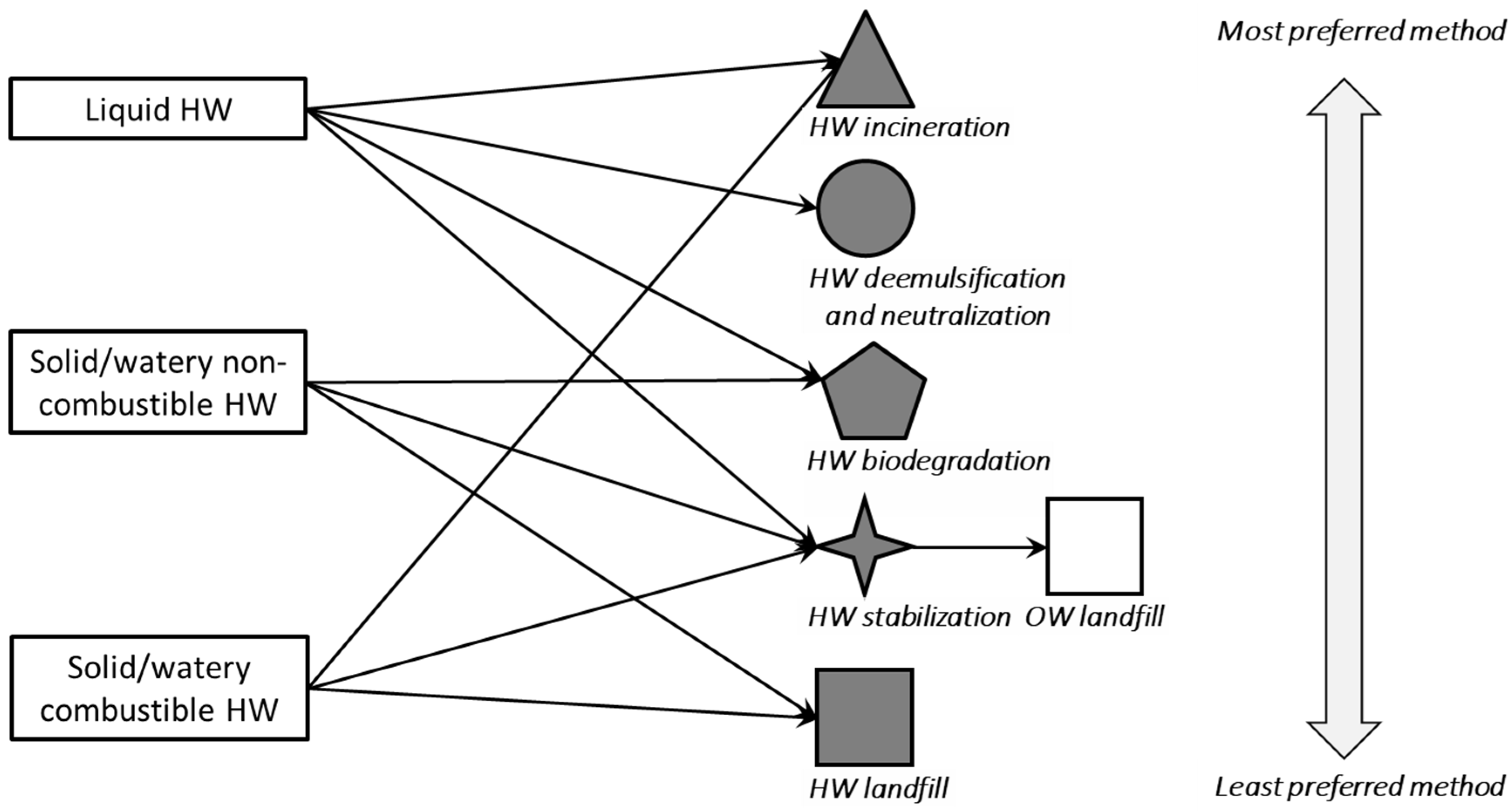
3.1. HW Treatment Methods
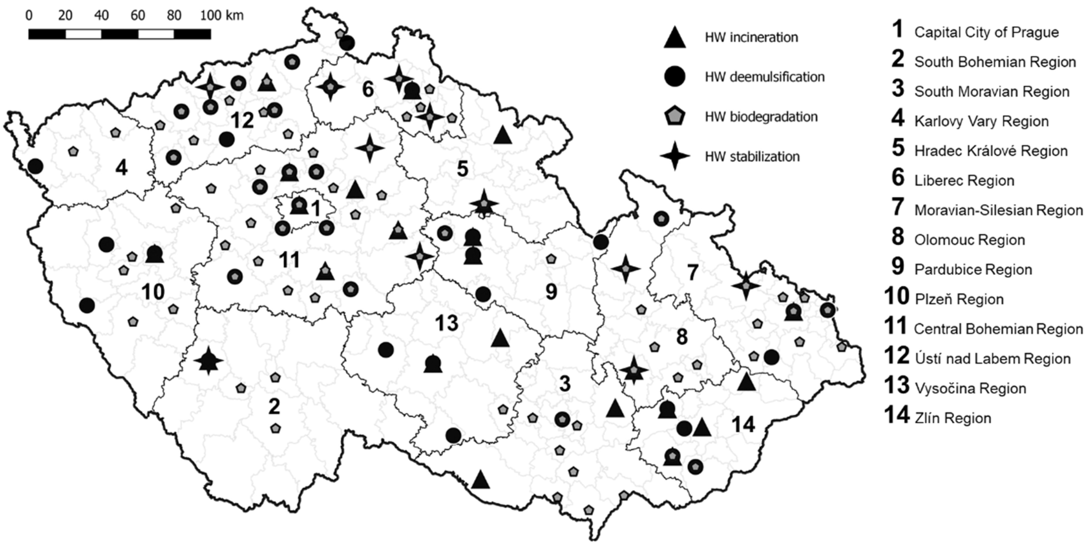
3.2. Inputs for the Case Study
- HW incinerator (163 waste catalogue codes).
- Demulsification unit (10 waste catalogue codes).
- Biodegradation unit (19 waste catalogue codes).
- Stabilization unit (115 waste catalogue codes).
- HW incinerator or stabilization unit (21 waste catalogue codes).
- Demulsification unit or stabilization unit (2 waste catalogue codes).
- Neutralization unit or stabilization unit (32 waste catalogue codes).
- Biodegradation unit or stabilization unit (11 waste catalogue codes).
4. Optimization
4.1. Assumptions
- HW incinerator, = 1.
- Industrial wastewater treatment, = 100.
- Stabilization unit, = 10,000.
- OW (non-hazardous), = 1,000,000.
- HW landfilling, = 1,000,000.
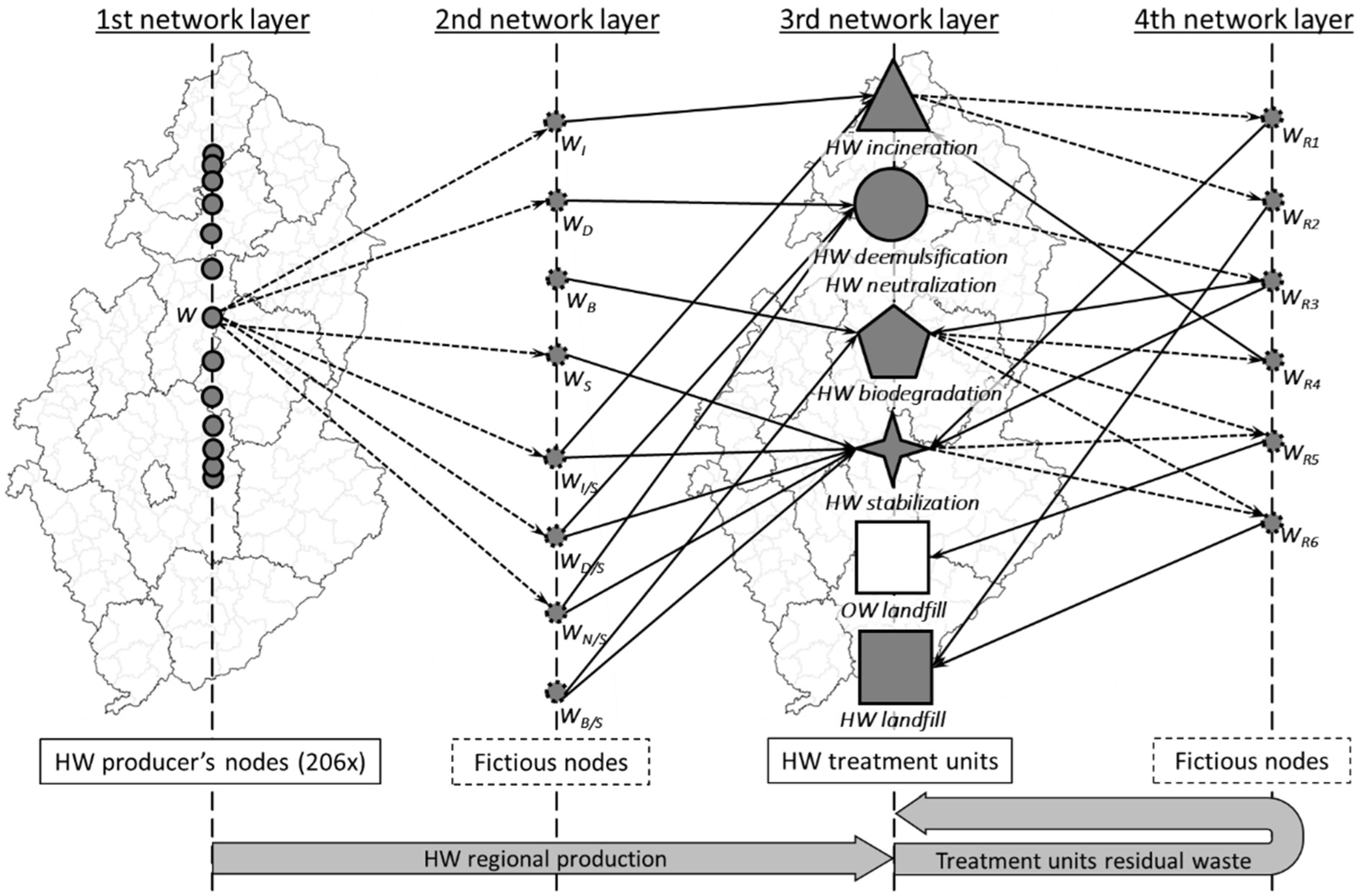
4.2. Selection of Network Type
4.3. Mathematical Model
| Sets: | |
| set of arcs (transportation infrastructure). | |
| set of nodes (waste producer—territorial unit). | |
| set of nodes in the 2nd network layer (waste producer—territorial unit). | |
| set of nodes in the 3rd network layer (HW treatment units—territorial unit). | |
| set of nodes in the 4th network layer (residual waste—territorial unit). | |
| Parameters: | |
| incidence matrix of transportation infrastructure, describes the existence of the arc between the second and third layers of the network, [-]. | |
| incidence matrix of residual waste, describes the connection between the third and fourth layers of the network, [-]. | |
| maximum available capacity of the unit [t/a]. | |
| coefficients of waste transformation, describes the amount of formed residual waste, [-]. | |
| weight penalization, describes the treatment preference, [EUR/t]. | |
| sum of transportation and processing costs, [EUR/t]. | |
| waste production in production nodes, [t/a]. | |
| Variables: | |
| used capacity of the unit, [t/a]. | |
| output (residuals) from the non-final units, [t/a]. | |
| waste amount, [t/a]. | |
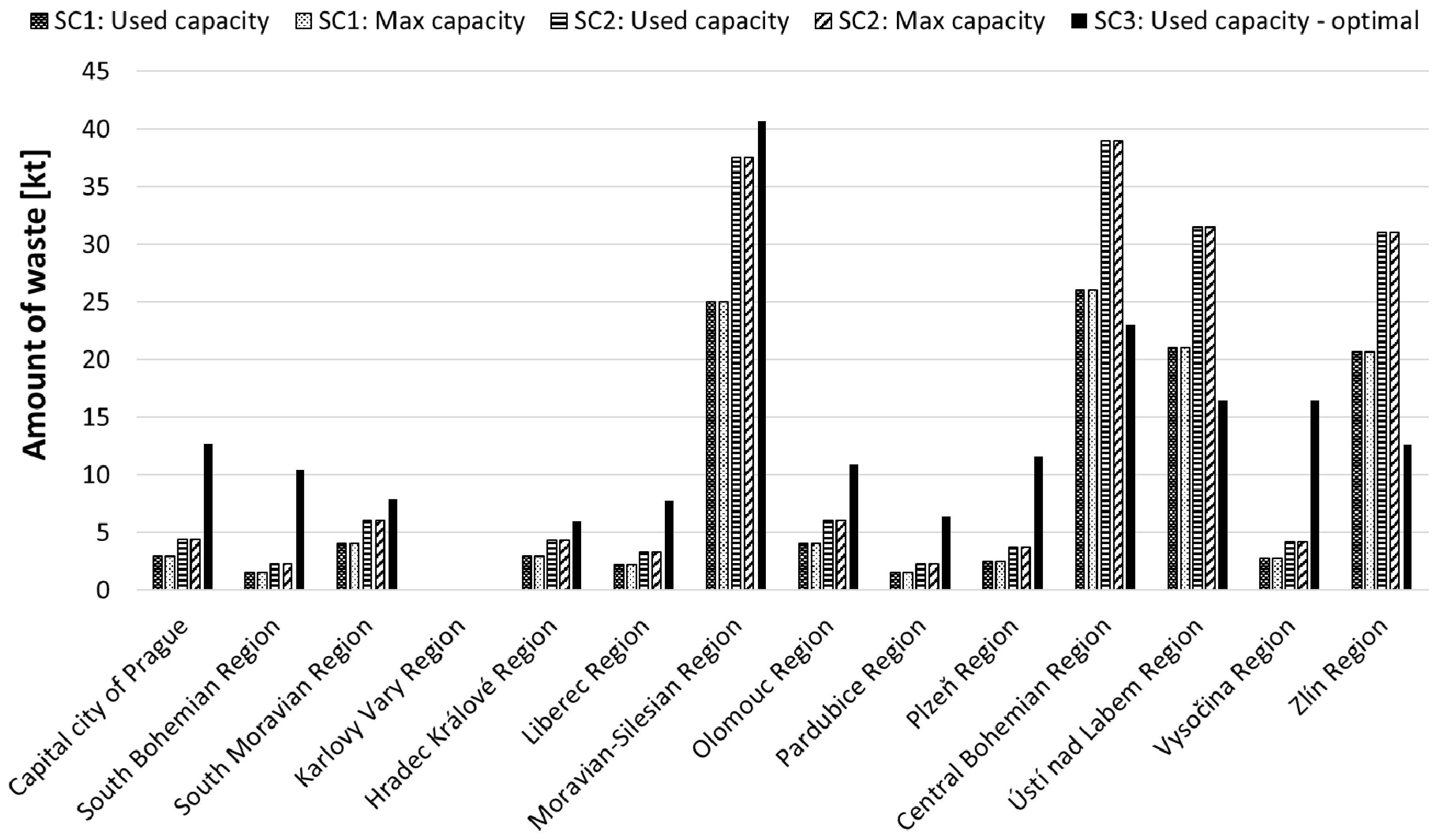
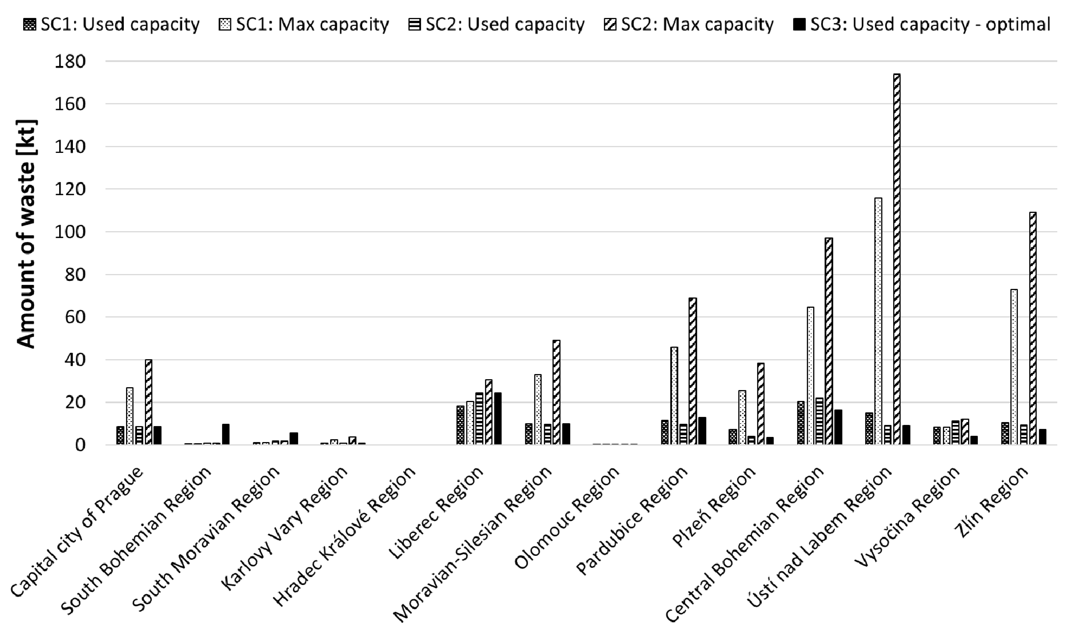
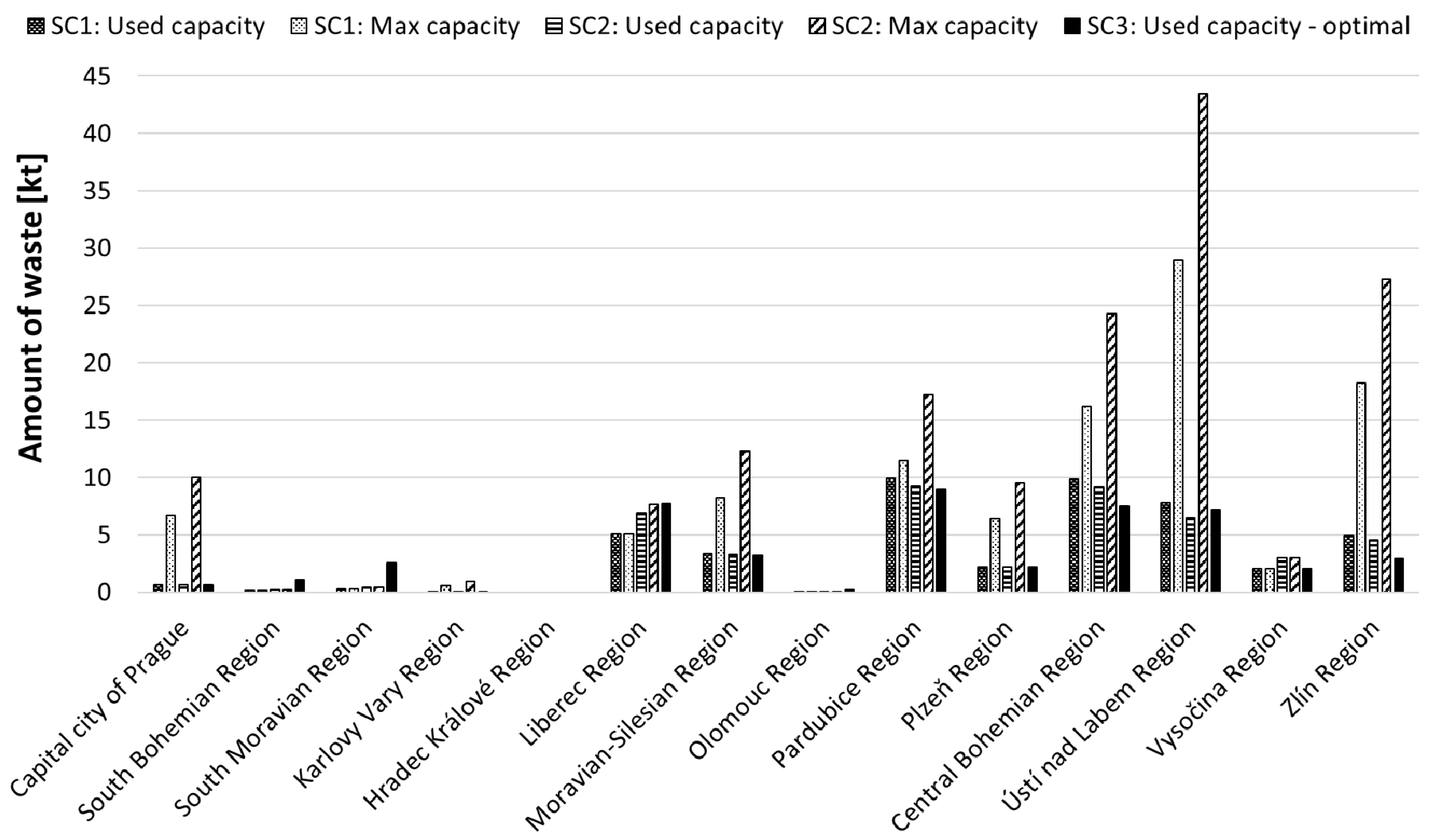
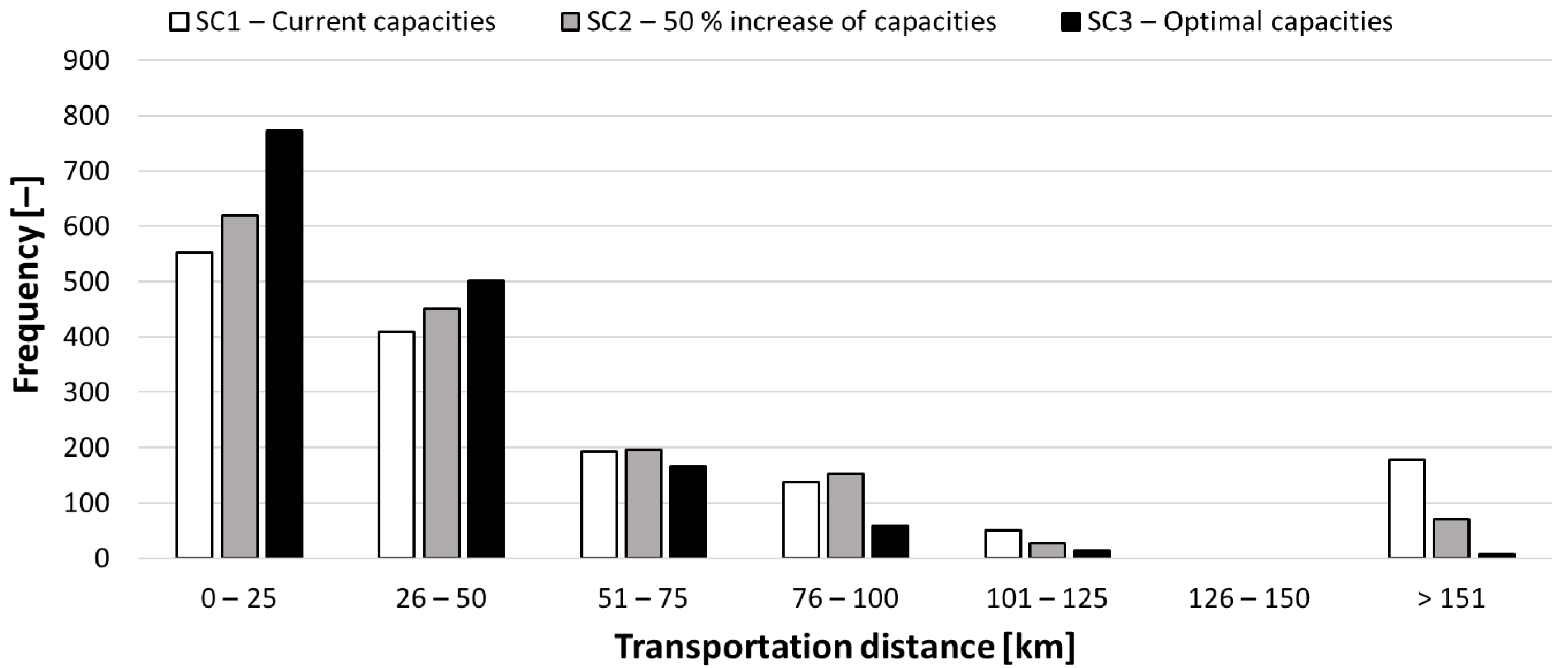
5. Results
- SC1—current processing capacity.
- SC2—increasing the processing capacity by 50%.
- SC3—unlimited capacities in existing locations.
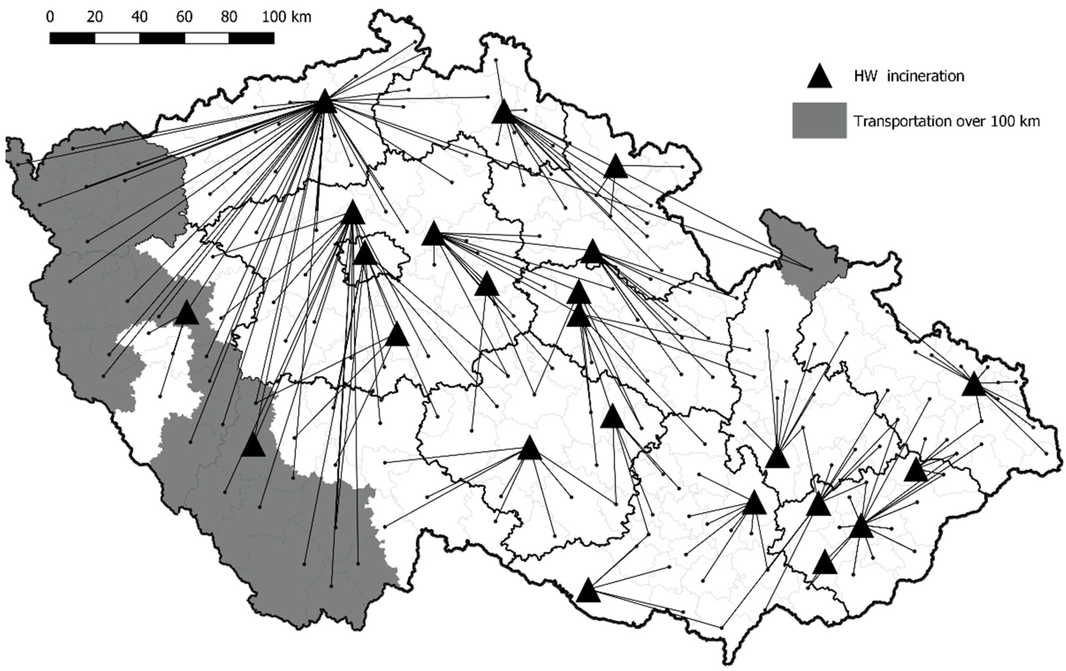
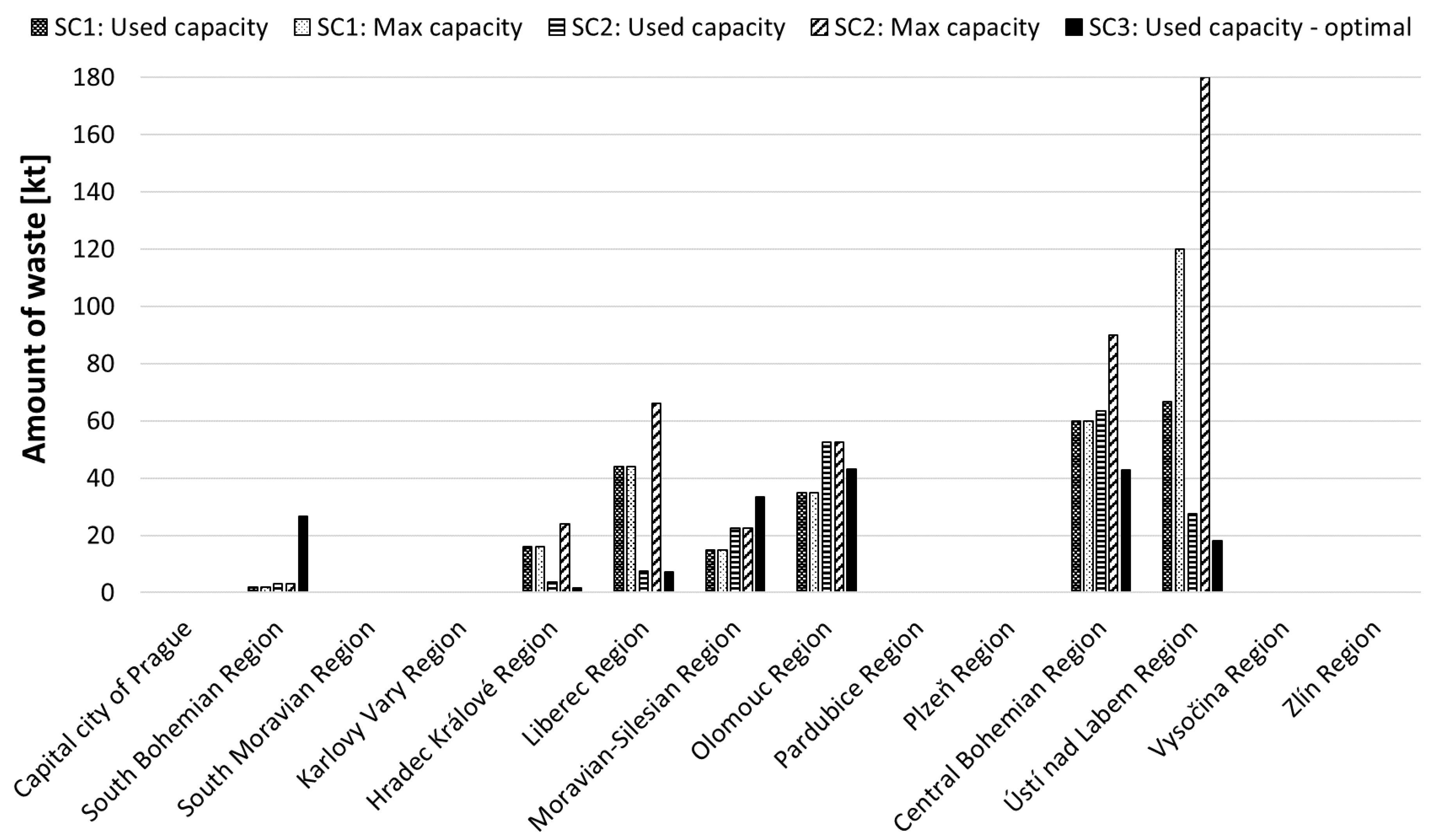
5.1. HW Thermal Treatment
5.2. Demulsification and Neutralization
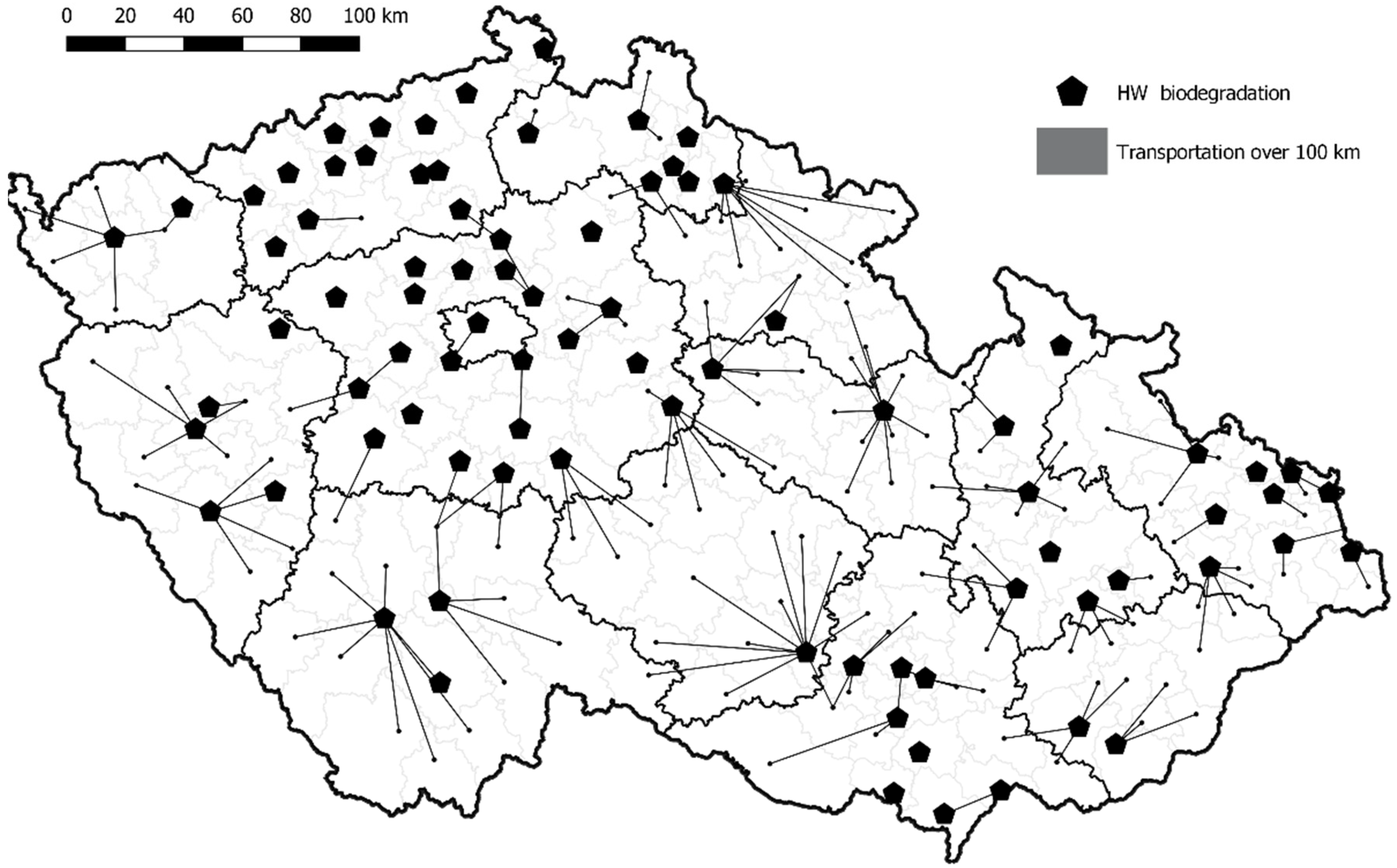
5.3. Biodegradation
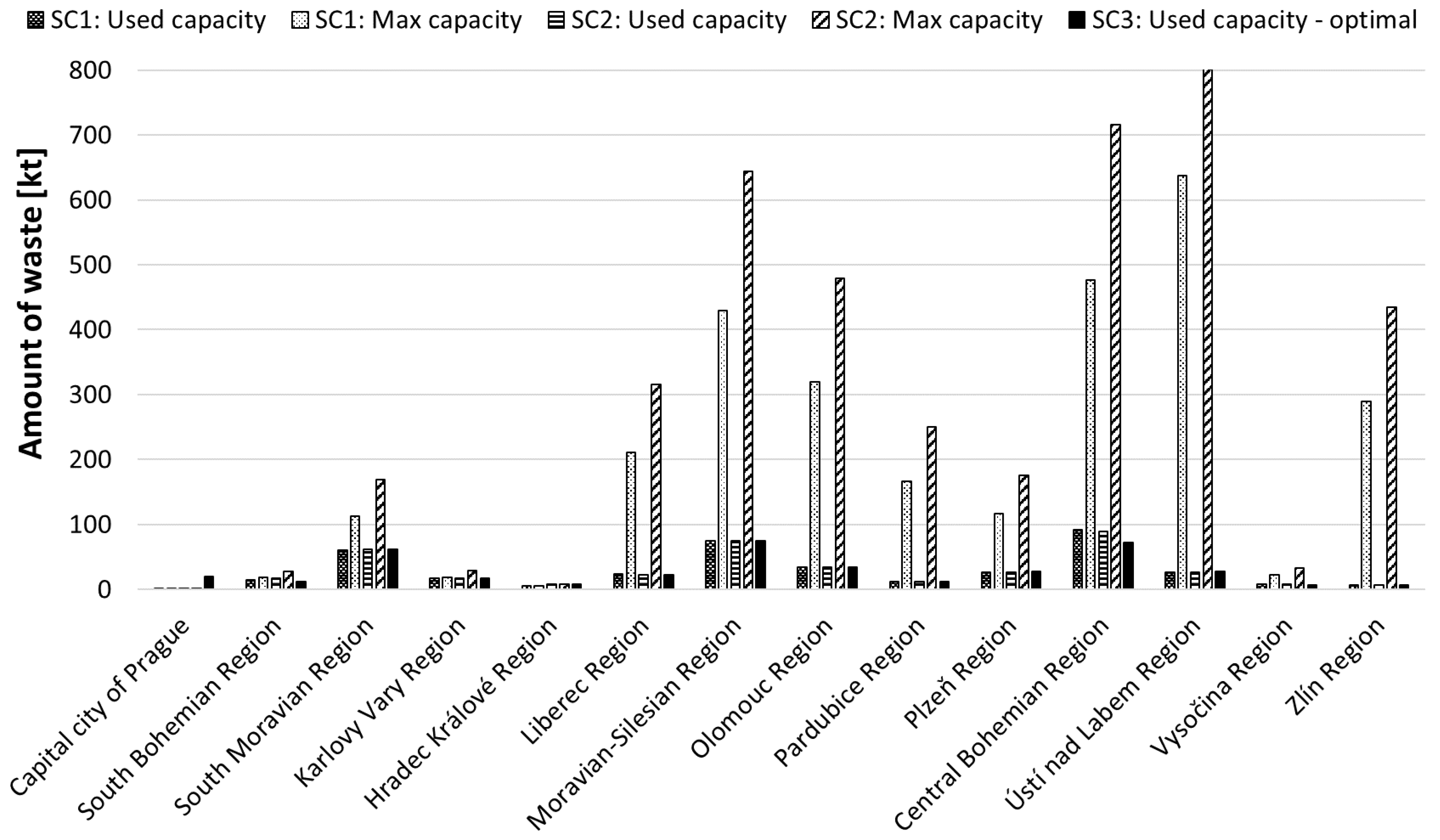
5.4. Stabilization
6. Results Summary and Recommendations
7. Conclusions
Author Contributions
Funding
Institutional Review Board Statement
Informed Consent Statement
Data Availability Statement
Acknowledgments
Conflicts of Interest
References
- Zhang, Z.; Malik, M.Z.; Khan, A.; Ali, N.; Malik, S.; Bilal, M. Environmental impacts of hazardous waste, and management strategies to reconcile circular economy and eco-sustainability. Sci. Total Environ. 2021, 807, 150856. [Google Scholar] [CrossRef]
- Ernst & Young. Podklady pro Oblast Podpory Odpadového a Oběhového Hospodářství OPŽP 2021–2027, Nebezpečné Odpady. 2020. Available online: https://www.mzp.cz/C1257458002F0DC7/cz/odpadove_obehove_hospodarstvi/$FILE/OODP-6_Nebezpecne_odpady-20200529.pdf (accessed on 10 February 2022). (In Czech).
- Pavlas, M.; Šomplák, R.; Smejkalová, V.; Nevrlý, V.; Zavíralová, L.; Kůdela, J.; Popela, P. Spatially distributed production data for supply chain models—Forecasting with hazardous waste. J. Clean. Prod. 2017, 161, 1317–1328. [Google Scholar] [CrossRef]
- Santoleri, J.; Reynolds, J.; Theodore, L. Introduction to Hazardous Waste Incineration, 2nd ed.; Wiley-Interscience: Hoboken, NJ, USA, 2000. [Google Scholar]
- Inglezakis, V.; Moustakas, K. Household hazardous waste management: A review. J. Environ. Manag. 2015, 150, 310–321. [Google Scholar] [CrossRef] [PubMed]
- Guerrero, L.A.; Maas, G.; Hogland, W. Solid waste management challenges for cities in developing countries. Waste Manag. 2013, 33, 220–232. [Google Scholar] [CrossRef]
- Sevilla, D.V.; López, A.F.; Bugallo, P.M.B. The Role of a Hazardous Waste Intermediate Management Plant in the Circularity of Products. Sustainability 2022, 14, 1241. [Google Scholar] [CrossRef]
- Barbosa-Póvoa, A.P.; da Silva, C.; Carvalho, A. Opportunities and challenges in sustainable supply chain: An operations research perspective. Eur. J. Oper. Res. 2018, 268, 399–431. [Google Scholar] [CrossRef]
- Kazemi, N.; Modak, N.; Govindan, K. A review of reverse logistics and closed loop supply chain management studies published in IJPR: A bibliometric and content analysis. Int. J. Prod. Res. 2019, 57, 4937–4960. [Google Scholar] [CrossRef] [Green Version]
- Court, C.D.; Munday, M.; Roberts, A.; Turner, K. Can hazardous waste supply chain ‘hotspots’ be identified using an input–output framework? Eur. J. Oper. Res. 2015, 241, 177–187. [Google Scholar] [CrossRef] [Green Version]
- Goldberg, D.M.; Hong, S. Minimizing the Risks of Highway Transport of Hazardous Materials. Sustainability 2019, 11, 6300. [Google Scholar] [CrossRef] [Green Version]
- Inghels, D.; Dullaert, W.; Vigo, D. A service network design model for multimodal municipal solid waste transport. Eur. J. Oper. Res. 2016, 254, 68–79. [Google Scholar] [CrossRef]
- Jiang, Y.; Zhang, Y. Supply Chain Optimization of Biodiesel Produced from Waste Cooking Oil. Transp. Res. Procedia 2016, 12, 938–949. [Google Scholar] [CrossRef] [Green Version]
- Zhao, J.; Huang, L.; Lee, D.-H.; Peng, Q. Improved approaches to the network design problem in regional hazardous waste management systems. Transp. Res. Part E Logist. Transp. Rev. 2016, 88, 52–75. [Google Scholar] [CrossRef]
- Chatzouridis, C.; Komilis, D. A methodology to optimally site and design municipal solid waste transfer stations using binary programming. Resour. Conserv. Recycl. 2012, 60, 89–98. [Google Scholar] [CrossRef]
- Lam, H.L.; Klemeš, J.J.; Kravanja, Z. Model-size reduction techniques for large-scale biomass production and supply networks. Energy 2011, 36, 4599–4608. [Google Scholar] [CrossRef]
- Pavlas, M.; Nevrlý, V.; Popela, P.; Šomplák, R. Heuristic for generation of waste transportation test networks. Mendel J. 2015, 21, 189–194. [Google Scholar]
- Nabavi-Pelesaraei, A.; Abdi, R.; Rafiee, S.; Bagheri, I. Determination of efficient and inefficient units for watermelon production-a case study: Guilan province of Iran. J. Saudi Soc. Agric. Sci. 2016, 15, 162–170. [Google Scholar] [CrossRef] [Green Version]
- Ziyuan, L.; Yingzhao, W.; Tianle, L.; Xiaoxue, W.; Wenzhuo, L.; Ying, Y.; Xiangfei, X. Double Path Optimization of Transport of Industrial Hazardous Waste Based on Green Supply Chain Management. Sustainability 2021, 13, 5215. [Google Scholar] [CrossRef]
- Wang, W.; Bao, J.; Yuan, S.; Zhou, H.; Li, G. Proposal for Planning an Integrated Management of Hazardous Waste: Chemical Park, Jiangsu Province, China. Sustainability 2019, 11, 2846. [Google Scholar] [CrossRef] [Green Version]
- Nabavi-Pelesaraei, A.; Bayat, R.; Hosseinzadeh-Bandbafha, H.; Afrasyabi, H.; Chau, K.W. Modeling of energy consumption and environmental life cycle assessment for incineration and landfill systems of municipal solid waste management—A case study in Tehran Metropolis of Iran. J. Clean. Prod. 2017, 148, 427–440. [Google Scholar] [CrossRef]
- Directive 2008/98/EC of the European Parliament and of the Council on Waste and Repealing Certain Directives. Off. J. Eur. Union 2008, L312, 3–30. Available online: https://eur-lex.europa.eu/legal-content/EN/TXT/PDF/?uri=CELEX:32008L0098&from=EN (accessed on 22 January 2022).
- Kropáč, J.; Bébar, L.; Pavlas, M. Industrial and hazardous waste combustion and energy production. Chem. Eng. Trans. 2012, 29, 673–678. [Google Scholar] [CrossRef]
- Rozumová, L.; Motyka, O.; Čabanová, K.; Seidlerová, J. Stabilization of waste bottom ash generated from hazardous waste incinerators. J. Environ. Chem. Eng. 2015, 3, 1–9. [Google Scholar] [CrossRef]
- Lombardi, L.; Carnevale, E.; Corti, A. A review of technologies and performances of thermal treatment systems for energy recovery from waste. Waste Manag. 2015, 37, 26–44. [Google Scholar] [CrossRef] [PubMed]
- Zolfaghari, R.; Fakhru’L-Razi, A.; Abdullah, L.C.; Elnashaie, S.S.; Pendashteh, A. Demulsification techniques of water-in-oil and oil-in-water emulsions in petroleum industry. Sep. Purif. Technol. 2016, 170, 377–407. [Google Scholar] [CrossRef]
- Rajakovic, V.; Aleksic, G.; Radetic, M.; Rajakovic, L. Efficiency of oil removal from real wastewater with different sorbent materials. J. Hazard. Mater. 2007, 143, 494–499. [Google Scholar] [CrossRef]
- Kundu, P.; Mishra, I.M. Removal of emulsified oil from oily wastewater (oil-in-water emulsion) using packed bed of polymeric resin beads. Sep. Purif. Technol. 2013, 118, 519–529. [Google Scholar] [CrossRef]
- Varshney, R.; Singh, P.; Yadav, D. Hazardous wastes treatment, storage, and disposal facilities. Hazard. Waste Manag. 2021, 2022, 33–64. [Google Scholar] [CrossRef]
- Lewandowski, G.A.; Filippi, L.J. Biological Treatment of Hazardous Waste; Wiley: New York, NY, USA, 1998. [Google Scholar]
- Singh, P.; Borthakur, A. A review on biodegradation and photocatalytic degradation of organic pollutants: A bibliometric and comparative analysis. J. Clean. Prod. 2018, 196, 1669–1680. [Google Scholar] [CrossRef]
- Chan, S.S.; Khoo, K.S.; Chew, K.W.; Ling, T.C.; Show, P.L. Recent advances biodegradation and biosorption of organic compounds from wastewater: Microalgae-bacteria consortium—A review. Bioresour. Technol. 2021, 344, 126159. [Google Scholar] [CrossRef]
- Zhou, X.; Zhou, M.; Wu, X.; Han, Y.; Geng, J.; Wang, T.; Wan, S.; Hou, H. Reductive solidification/stabilization of chromate in municipal solid waste incineration fly ash by ascorbic acid and blast furnace slag. Chemosphere 2017, 182, 76–84. [Google Scholar] [CrossRef]
- Park, Y.J. Stabilization of a chlorine-rich fly ash by colloidal silica solution. J. Hazard. Mater. 2009, 162, 819–822. [Google Scholar] [CrossRef] [PubMed]
- Vavva, C.; Voutsas, E.; Magoulas, K. Process development for chemical stabilization of fly ash from municipal solid waste incineration. Chem. Eng. Res. Des. 2017, 125, 57–71. [Google Scholar] [CrossRef]
- Ho, L.T.; Van Echelpoel, W.; Goethals, P.L. Design of waste stabilization pond systems: A review. Water Res. 2017, 123, 236–248. [Google Scholar] [CrossRef] [PubMed]
- De Feo, G.; De Gisi, S. Using MCDA and GIS for hazardous waste landfill siting considering land scarcity for waste disposal. Waste Manag. 2014, 34, 2225–2238. [Google Scholar] [CrossRef] [PubMed]
- CENIA. Waste Management Information System for Czech Republic. 2022. Available online: https://www.cenia.cz/odpadove-a-obehove-hospodarstvi/isoh/ (accessed on 16 February 2022).
- Gregor, J.; Šomplák, R.; Pavlas, M. Transportation cost as an integral part of supply chain optimization in the field of waste management. Chem. Eng. Trans. 2017, 56, 1927–1932. [Google Scholar] [CrossRef]
- GAMS Documentation. Solver Manuals, CPLEX 12. Available online: https://www.gams.com/33/docs/S_CPLEX.html (accessed on 16 February 2022).
- Ren, X.; Che, Y.; Yang, K.; Tao, Y. Risk perception and public acceptance toward a highly protested Waste-to-Energy facility. Waste Manag. 2016, 48, 528–539. [Google Scholar] [CrossRef] [PubMed]


| HW Sub-Stream | 2018 | 2025 | 2030 | 2035 |
|---|---|---|---|---|
| Incineration | 83,140 | 84,049 | 90,799 | 97,096 |
| Demulsification | 0 | 2 | 2 | 2 |
| Biodegradation | 323 | 1192 | 1140 | 1063 |
| Stabilization | 166,829 | 153,502 | 151,599 | 150,496 |
| Combustion or stabilization | 86,097 | 88,487 | 94,650 | 100,283 |
| Demulsification or stabilization | 83,721 | 101,307 | 110,615 | 118,732 |
| Neutralization or stabilization | 45,553 | 44,130 | 46,148 | 48,132 |
| Biodegradation or stabilization | 572,249 | 410,685 | 379,229 | 344,630 |
| Total | 1,037,912 | 883,354 | 874,182 | 860,434 |
| Waste Treatment Technology | Residual Waste | Residual Waste Production (% Weight of Input Waste) | Residual Waste Final Treatment |
|---|---|---|---|
| Incineration | Bottom ash | 20 | HW or OW landfill |
| Incineration | Fly ash | 5 | Stabilization |
| Demulsification | Sludge | 5 | Biodegradation or stabilization |
| Neutralization | Neutralized sludge | 5 | Stabilization |
| Biodegradation | Combustible gas | 5 | Incineration |
| Biodegradation | Biodegraded waste | 65 | HW or OW landfill |
| Stabilization | Stabilized waste | 70 | OW landfill |
| Stabilization | HW | 70 | HW landfill |
| HW Treatment Type | Incineration | Demulsification | Neutralization | Biodegradation | Stabilization | |||||
|---|---|---|---|---|---|---|---|---|---|---|
| <100 km | >100 km | <100 km | >100 km | <100 km | >100 km | <100 km | >100 km | <100 km | >100 km | |
| Incineration | 1 | 10,000 | - | - | - | - | - | - | - | - |
| Demulsification | - | - | 100 | 10,000 | - | - | - | - | - | - |
| Biodegradation | - | - | - | - | - | - | 100 | 10,000 | - | - |
| Stabilization | - | - | - | - | - | - | - | - | 10,000 | 10,000 |
| Combustion or stabilization | 1 | 10,000 | - | - | - | - | - | - | 10,000 | 10,000 |
| Demulsification or stabilization | - | - | 100 | 10,000 | - | - | - | - | 10,000 | 10,000 |
| Neutralization or stabilization | - | - | - | - | 100 | 10,000 | - | - | 10,000 | 10,000 |
| Biodegradation or stabilization | - | - | - | - | - | - | 100 | 10,000 | 10,000 | 10,000 |
Publisher’s Note: MDPI stays neutral with regard to jurisdictional claims in published maps and institutional affiliations. |
© 2022 by the authors. Licensee MDPI, Basel, Switzerland. This article is an open access article distributed under the terms and conditions of the Creative Commons Attribution (CC BY) license (https://creativecommons.org/licenses/by/4.0/).
Share and Cite
Šomplák, R.; Kropáč, J.; Pluskal, J.; Pavlas, M.; Urbánek, B.; Vítková, P. A Multi-Commodity Mathematical Modelling Approach—Hazardous Waste Treatment Infrastructure Planning in the Czech Republic. Sustainability 2022, 14, 3536. https://0-doi-org.brum.beds.ac.uk/10.3390/su14063536
Šomplák R, Kropáč J, Pluskal J, Pavlas M, Urbánek B, Vítková P. A Multi-Commodity Mathematical Modelling Approach—Hazardous Waste Treatment Infrastructure Planning in the Czech Republic. Sustainability. 2022; 14(6):3536. https://0-doi-org.brum.beds.ac.uk/10.3390/su14063536
Chicago/Turabian StyleŠomplák, Radovan, Jiří Kropáč, Jaroslav Pluskal, Martin Pavlas, Boris Urbánek, and Petra Vítková. 2022. "A Multi-Commodity Mathematical Modelling Approach—Hazardous Waste Treatment Infrastructure Planning in the Czech Republic" Sustainability 14, no. 6: 3536. https://0-doi-org.brum.beds.ac.uk/10.3390/su14063536