
Analysis of the Relationship between the Characteristics of the Areas of Influence of Bus Stops and the Decrease in Ridership during COVID-19 Lockdowns

 , , and
Abstract
:1. Introduction
1.1. Context and Literature Review
1.2. Objectives and Contributions
1.3. COVID-19 Spread and Lockdown Regulations in Spain and Galicia
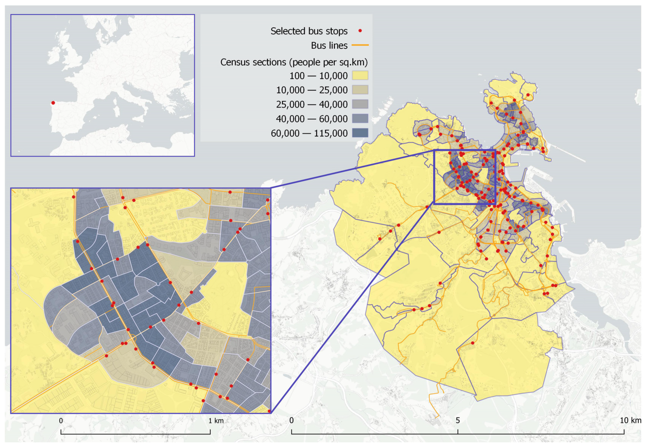
2. Data Processing and Spatial Analysis
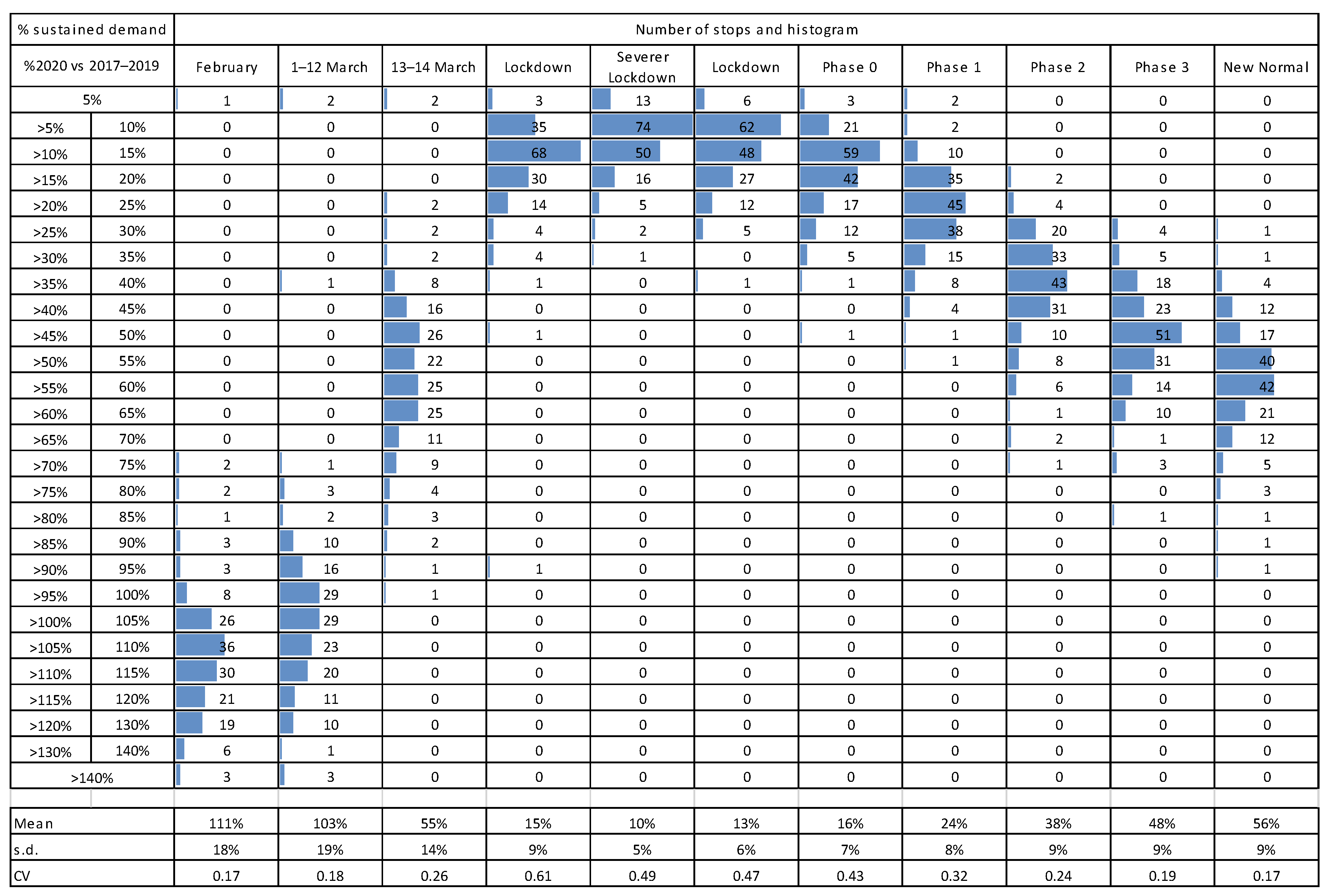
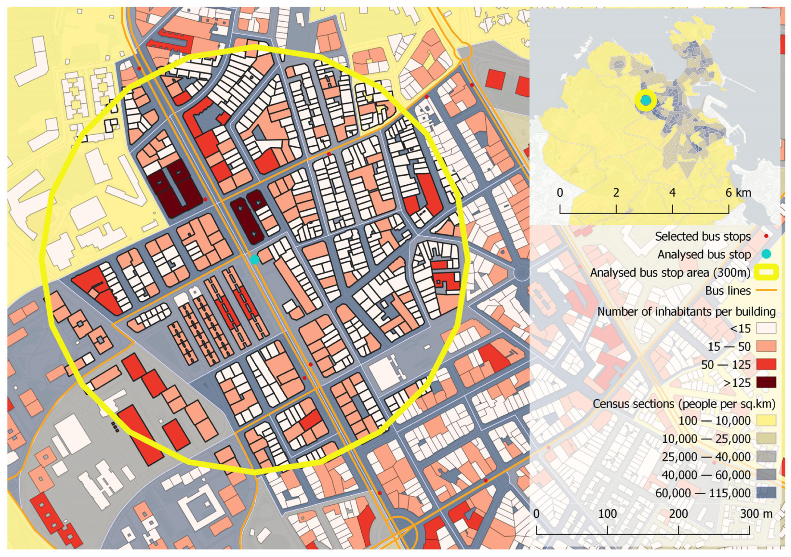
2.1. Selection of Bus Stops and Time Periods
- -
- February (normal situation)
- -
- 1–12 March (normal situation, but influenced by information about the pandemic in Italy and certain Spanish regions)
- -
- 13–14 March (state of alarm announced, first teaching activity restrictions)
- -
- 15–27 March (lockdown)
- -
- 28 March–9 April (severer lockdown)
- -
- 10 April–3 May (lockdown)
- -
- 4–10 May (Phase 0)
- -
- 11–24 May (Phase 1)
- -
- 25 May–7 June (Phase 2)
- -
- 8–14 June (Phase 3)
- -
- 15–30 June (new normal)
2.2. Data Sources and Variable Description
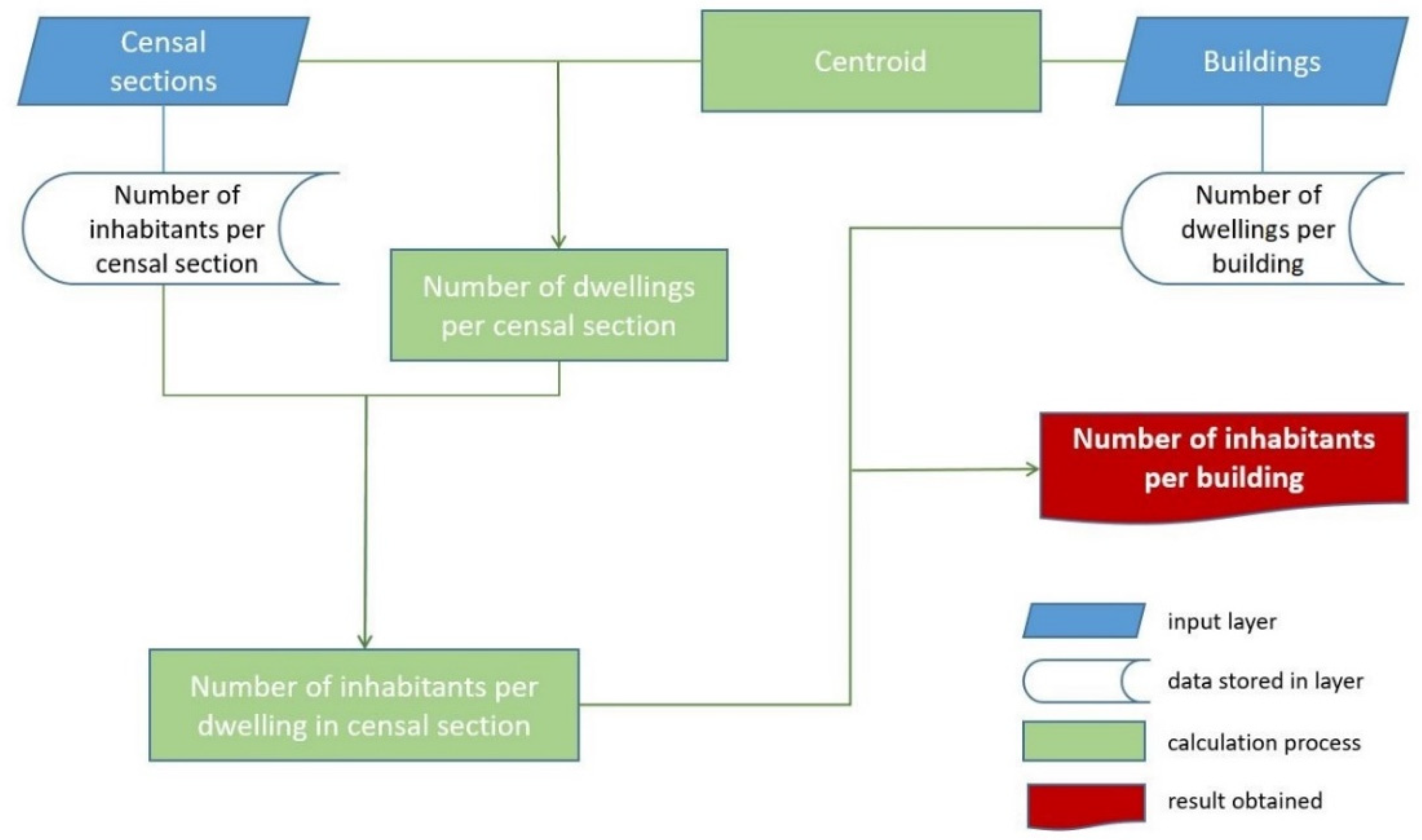
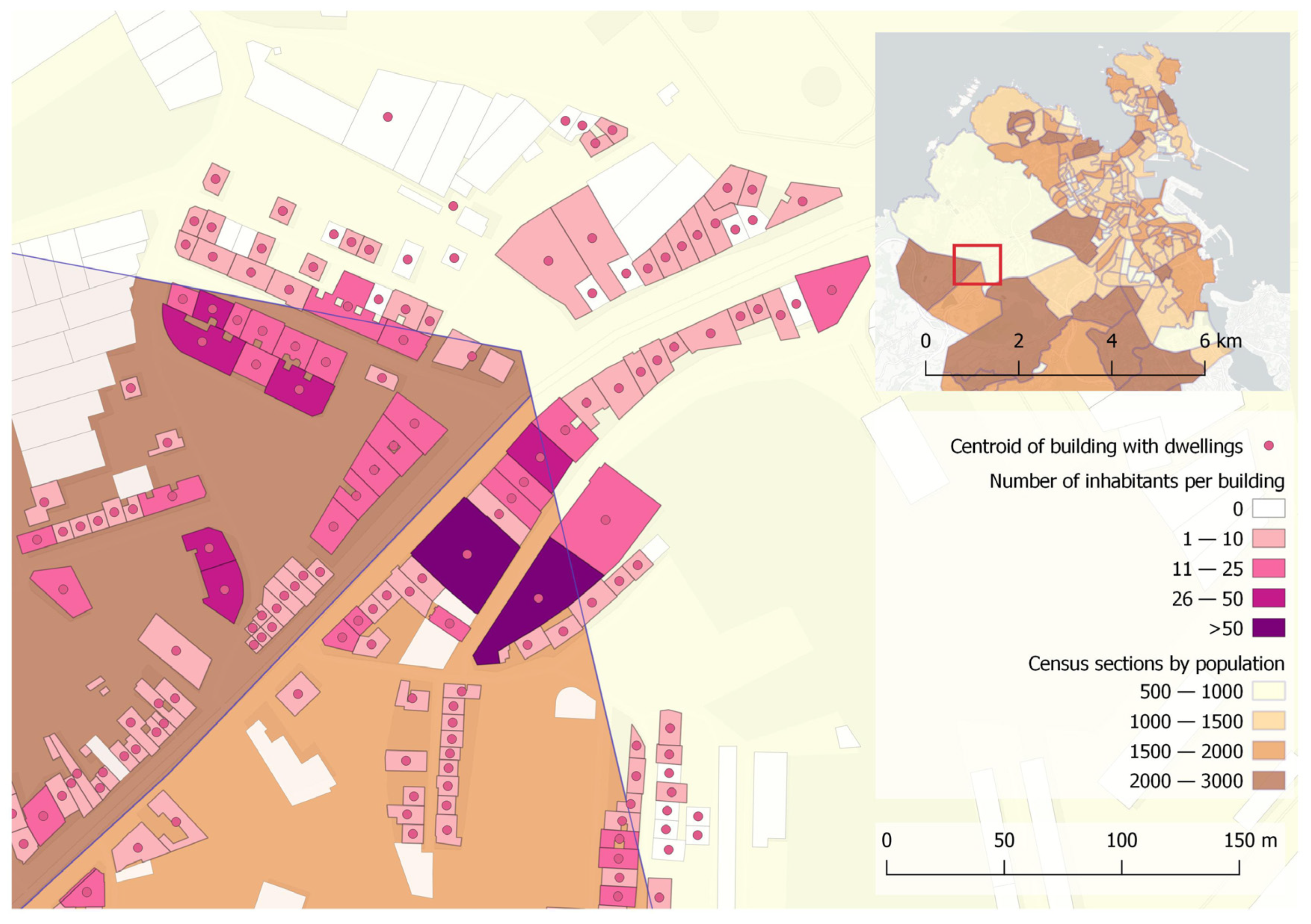
2.3. GIS Data Processing
3. Modelling and Discussion
4. Conclusions
Author Contributions
Funding
Institutional Review Board Statement
Informed Consent Statement
Acknowledgments
Conflicts of Interest
References
- Listings of WHO’s Response to COVID-19. Available online: https://www.who.int/news/item/29-06-2020-covidtimeline (accessed on 8 June 2021).
- Kraemer, M.U.G.; Yang, C.H.; Gutierrez, B.; Wu, C.H.; Klein, B.; Pigott, D.M.; du Plessis, L.; Faria, N.R.; Li, R.; Hanage, W.P.; et al. The effect of human mobility and control measures on the COVID-19 epidemic in China. Science 2020, 368, 493–497. [Google Scholar] [CrossRef] [PubMed] [Green Version]
- Mogaji, E. Impact of COVID-19 on transportation in Lagos, Nigeria. Transp. Res. Interdiscip. Perspect. 2020, 6, 100154. [Google Scholar] [CrossRef] [PubMed]
- Al-Awadhi, A.M.; Alsaifi, K.; Al-Awadhi, A.; Alhammadi, S. Death and contagious infectious diseases: Impact of the COVID-19 virus on stock market returns. J. Behav. Exp. Financ. 2020, 27, 100326. [Google Scholar] [CrossRef] [PubMed]
- Bonaccorsi, G.; Pierri, F.; Cinelli, M.; Flori, A.; Galeazzi, A.; Porcelli, F.; Schmidt, A.L.; Valensise, C.M.; Scala, A.; Quattrociocchi, W.; et al. Economic and social consequences of human mobility restrictions under COVID-19. Proc. Natl. Acad. Sci. USA 2020, 117, 15530–15535. [Google Scholar] [CrossRef] [PubMed]
- Mazza, C.; Ricci, E.; Biondi, S.; Colasanti, M.; Ferracuti, S.; Napoli, C.; Roma, P. A Nationwide Survey of Psychological Distress among Italian People during the COVID-19 Pandemic: Immediate Psychological Responses and Associated Factors. Int. J. Environ. Res. Public Health 2020, 17, 3165. [Google Scholar] [CrossRef] [PubMed]
- Qiu, J.; Shen, B.; Zhao, M.; Wang, Z.; Xie, B.; Xu, Y. A nationwide survey of psychological distress among Chinese people in the COVID-19 epidemic: Implications and policy recommendations. Gen. Psychiatry 2020, 33, e100213. [Google Scholar] [CrossRef] [Green Version]
- Le Quéré, C.; Jackson, R.B.; Jones, M.W.; Smith, A.J.P.; Abernethy, S.; Andrew, R.M.; De-Gol, A.J.; Willis, D.R.; Shan, Y.; Canadell, J.G.; et al. Temporary reduction in daily global CO2 emissions during the COVID-19 forced confinement. Nat. Clim. Chang. 2020, 10, 647–653. [Google Scholar] [CrossRef]
- Orro, A.; Novales, M.; Monteagudo, Á.; Pérez-López, J.B.; Bugarín, M.R. Impact on city bus transit services of the COVID-19 lockdown and return to the new normal: The case of A Coruña (Spain). Sustainbility 2020, 12, 7206. [Google Scholar] [CrossRef]
- Munawar, H.S.; Khan, S.I.; Qadir, Z.; Kouzani, A.Z.; Mahmud, M.A.P. Insight into the impact of COVID-19 on Australian transportation sector: An economic and community-based perspective. Sustainbility 2021, 13, 1276. [Google Scholar] [CrossRef]
- Aloi, A.; Alonso, B.; Benavente, J.; Cordera, R.; Echániz, E.; González, F.; Ladisa, C.; Lezama-Romanelli, R.; López-Parra, Á.; Mazzei, V.; et al. Effects of the COVID-19 lockdown on urban mobility: Empirical evidence from the city of Santander (Spain). Sustainbility 2020, 12, 3870. [Google Scholar] [CrossRef]
- Liu, L.; Miller, H.J.; Scheff, J. The impacts of COVID-19 pandemic on public transit demand in the United States. PLoS ONE 2020, 15, e0242476. [Google Scholar] [CrossRef] [PubMed]
- Kim, J.; Kwan, M.-P. The impact of the COVID-19 pandemic on people’s mobility: A longitudinal study of the U.S. from March to September of 2020. J. Transp. Geogr. 2021, 93, 103039. [Google Scholar] [CrossRef]
- Allcott, H.; Boxell, L.; Conway, J.; Gentzkow, M.; Thaler, M.; Yang, D. Polarization and public health: Partisan differences in social distancing during the coronavirus pandemic. J. Public Econ. 2020, 191, 104254. [Google Scholar] [CrossRef] [PubMed]
- Grossman, G.; Kim, S.; Rexer, J.M.; Thirumurthy, H. Political partisanship influences behavioral responses to governors’ recommendations for COVID-19 prevention in the United States. Proc. Natl. Acad. Sci. USA 2020, 117, 24144–24153. [Google Scholar] [CrossRef] [PubMed]
- Hart, P.S.; Chinn, S.; Soroka, S. Politicization and Polarization in COVID-19 News Coverage. Sci. Commun. 2020, 42, 679–697. [Google Scholar] [CrossRef]
- Habib, K.N.; Hawkins, J.; Shakib, S.; Loa, P.; Mashrur, S.; Dianat, A.; Wang, K.; Hossain, S.; Liu, Y.Y. Assessing the impacts of COVID-19 on urban passenger travel demand in the greater Toronto area: Description of a multi-pronged and multi-staged study with initial results. Transp. Lett. 2021, 13, 353–366. [Google Scholar] [CrossRef]
- Bajos, N.; Jusot, F.; Pailhé, A.; Spire, A.; Martin, C.; Meyer, L.; Lydié, N.; Franck, J.-E.; Zins, M.; Carrat, F. When lockdown policies amplify social inequalities in COVID-19 infections: Evidence from a cross-sectional population-based survey in France. BMC Public Health 2021, 21, 705. [Google Scholar] [CrossRef]
- Benítez, M.A.; Velasco, C.; Sequeira, A.R.; Henríquez, J.; Menezes, F.M.; Paolucci, F. Responses to COVID-19 in five Latin American countries. Health Policy Technol. 2020, 9, 525–559. [Google Scholar] [CrossRef]
- Chan, E.Y.Y.; Huang, Z.; Lo, E.S.K.; Hung, K.K.C.; Wong, E.L.Y.; Wong, S.Y.S. Sociodemographic predictors of health risk perception, attitude and behavior practices associated with health-emergency disaster risk management for biological hazards: The case of COVID-19 pandemic in Hong Kong, SAR China. Int. J. Environ. Res. Public Health 2020, 17, 3869. [Google Scholar] [CrossRef]
- Nicola, M.; Alsafi, Z.; Sohrabi, C.; Kerwan, A.; Al-Jabir, A.; Iosifidis, C.; Agha, M.; Agha, R. The Socio-Economic Implications of the Coronavirus Pandemic (COVID-19): A Review. Int. J. Surg. 2020, 78, 185–193. [Google Scholar] [CrossRef]
- Niedzwiedz, C.L.; O’Donnell, C.A.; Jani, B.D.; Demou, E.; Ho, F.K.; Celis-Morales, C.; Nicholl, B.I.; Mair, F.S.; Welsh, P.; Sattar, N.; et al. Ethnic and socioeconomic differences in SARS-CoV-2 infection: Prospective cohort study using UK Biobank. BMC Med. 2020, 18, 160. [Google Scholar] [CrossRef]
- Dueñas, M.; Campi, M.; Olmos, L.E. Changes in mobility and socioeconomic conditions during the COVID-19 outbreak. Humanit. Soc. Sci. Commun. 2021, 8, 101. [Google Scholar] [CrossRef]
- Hu, S.; Chen, P. Who left riding transit? Examining socioeconomic disparities in the impact of COVID-19 on ridership. Transp. Res. Part D Transp. Environ. 2021, 90, 102654. [Google Scholar] [CrossRef]
- Kim, S.; Lee, S.; Ko, E.; Jang, K.; Yeo, J. Changes in car and bus usage amid the COVID-19 pandemic: Relationship with land use and land price. J. Transp. Geogr. 2021, 96, 103168. [Google Scholar] [CrossRef] [PubMed]
- Currie, G.; Ahern, A.; Delbosc, A. Exploring the drivers of light rail ridership: An empirical route level analysis of selected Australian, North American and European systems. Transportation 2011, 38, 545–560. [Google Scholar] [CrossRef] [Green Version]
- Cervero, R.; Murakami, J.; Miller, M.A. Direct Ridership Model of Bus Rapid Transit in Los Angeles County. Transp. Res. Rec. 2010, 2145, 1–7. [Google Scholar] [CrossRef] [Green Version]
- Diab, E.; Kasraian, D.; Miller, E.J.; Shalaby, A. The rise and fall of transit ridership across Canada: Understanding the determinants. Transp. Policy 2020, 96, 101–112. [Google Scholar] [CrossRef]
- Coronavirus (COVID-19)—15 de Marzo 2020|DSN. Available online: https://www.dsn.gob.es/es/actualidad/sala-prensa/coronavirus-covid-19-15-marzo-2020 (accessed on 29 April 2021).
- La Moncloa. 13 March 2020. El Gobierno Declarará Mañana el Estado de Alarma por el Coronavirus [Presidente/Destacados]. Available online: https://www.lamoncloa.gob.es/presidente/actividades/Paginas/2020/130320-sanchez-declaracio.aspx (accessed on 12 July 2021).
- Real Decreto 463/2020, de 14 de Marzo, por el que se Declara el Estado de Alarma para la Gestión de la Situación de Crisis Sanitaria Ocasionada por el COVID-19. Available online: https://www.boe.es/eli/es/rd/2020/03/14/463 (accessed on 25 June 2021).
- Real Decreto 487/2020, de 10 de Abril, por el que se Prorroga el Estado de Alarma Declarado por el Real Decreto 463/2020, de 14 de Marzo, por el Que se Declara el Estado de Alarma para la Gestión de la Situación de Crisis Sanitaria Ocasionada por el COVID-19. Available online: https://www.boe.es/buscar/doc.php?id=BOE-A-2020-4413 (accessed on 12 July 2021).
- Real Decreto 492/2020, de 24 de Abril, por el que se Prorroga el Estado de Alarma Declarado por el Real Decreto 463/2020, de 14 de Marzo, por el que se Declara el Estado de Alarma para la Gestión de la Situación de Crisis Sanitaria Ocasionada por el COVID-19. Available online: https://www.boe.es/buscar/doc.php?id=BOE-A-2020-4652 (accessed on 12 July 2021).
- Real Decreto 514/2020, de 8 de Mayo, por el que se Prorroga el Estado de Alarma Declarado por el Real Decreto 463/2020, de 14 de Marzo, por el que se Declara el Estado de Alarma para la Gestión de la Situación de Crisis Sanitaria Ocasionada por el COVID-19. Available online: https://www.boe.es/buscar/doc.php?id=BOE-A-2020-4902 (accessed on 12 July 2021).
- Real Decreto 537/2020, de 22 de Mayo, por el que se Prorroga el Estado de Alarma Declarado por el Real Decreto 463/2020, de 14 de Marzo, por el que se Declara el Estado de Alarma para la Gestión de la Situación de Crisis Sanitaria Ocasionada por el COVID-19. Available online: https://www.boe.es/buscar/act.php?id=BOE-A-2020-5243 (accessed on 12 July 2021).
- Real Decreto 476/2020, de 27 de Marzo, por el que se Prorroga el Estado de Alarma Declarado por el Real Decreto 463/2020, de 14 de Marzo, por el que se Declara el Estado de Alarma para la Gestión de la Situación de Crisis Sanitaria Ocasionada por el COVID-19. Available online: https://www.boe.es/buscar/act.php?id=BOE-A-2020-4155 (accessed on 12 July 2021).
- La Moncloa. 28/04/2020. El Gobierno Aprueba un Plan de Desescalada que se Prolongará Hasta Finales de Junio [Consejo de Ministros/Resúmenes]. Available online: https://www.lamoncloa.gob.es/consejodeministros/resumenes/Paginas/2020/280420-consejo_ministros.aspx (accessed on 12 July 2021).
- Orden SND/386/2020, de 3 de Mayo, por la que se Flexibilizan Determinadas Restricciones Sociales y se Determinan las Condiciones de Desarrollo de la Actividad de Comercio Minorista y de Prestación de Servicios, así como de las Actividades de Hostelería y. Available online: https://www.boe.es/buscar/doc.php?id=BOE-A-2020-4791 (accessed on 12 July 2021).
- Orden SND/399/2020, de 9 de Mayo, para la Flexibilización de Determinadas Restricciones de Ámbito Nacional, Establecidas tras la Declaración del Estado de Alarma en Aplicación de la fase 1 del Plan para la Transición Hacia una Nueva Normalidad. Available online: https://www.boe.es/buscar/doc.php?id=BOE-A-2020-4911 (accessed on 12 July 2021).
- Orden SND/414/2020, de 16 de Mayo, para la Flexibilización de Determinadas Restricciones de Ámbito Nacional Establecidas tras la Declaración del Estado de Alarma en Aplicación de la Fase 2 del Plan para la Transición Hacia una Nueva Normalidad. Available online: https://www.boe.es/buscar/doc.php?id=BOE-A-2020-5088 (accessed on 12 July 2021).
- Orden SND/458/2020, de 30 de Mayo, para la Flexibilización de Determinadas Restricciones de Ámbito Nacional Establecidas tras la Declaración del Estado de Alarma en Aplicación de la Fase 3 del Plan para la Transición Hacia una Nueva Normalidad. Available online: https://www.boe.es/buscar/act.php?id=BOE-A-2020-5469 (accessed on 12 July 2021).
- DECRETO 88/2020, de 8 de junio, por el que se Adoptan Medidas en Materia de ocio Nocturno de Aplicación en el Ámbito Territorial de la Comunidad Autónoma de Galicia Durante la Fase 3 del Plan para la Transición Hacia una Nueva Normalidad. Available online: https://www.xunta.gal/dog/Publicados/excepcional/2020/20200608/2331/AnuncioC3B0-080620-1_gl.html (accessed on 12 July 2021).
- Resolución do DOG no 111 do 9 June 2020—Xunta de Galicia. Available online: https://www.xunta.gal/dog/Publicados/2020/20200609/AnuncioG0533-010620-0001_gl.html (accessed on 28 February 2022).
- Resolución del DOG no 115 de 13 June 2020—Xunta de Galicia. Available online: https://www.xunta.gal/dog/Publicados/2020/20200613/AnuncioC3K1-120620-1_es.html (accessed on 12 July 2021).
- Real Decreto 555/2020, de 5 de Junio, por el que se Prorroga el Estado de Alarma Declarado por el Real Decreto 463/2020, de 14 de Marzo, por el que se Declara el Estado de Alarma para la Gestión de la Situación de Crisis Sanitaria Ocasionada por el COVID-19. Available online: https://www.boe.es/buscar/act.php?id=BOE-A-2020-5767 (accessed on 12 July 2021).
- La Moncloa. Estado de Alarma. Available online: https://www.lamoncloa.gob.es/covid-19/Paginas/estado-de-alarma.aspx (accessed on 12 July 2021).
- INE. Instituto Nacional de Estadística. Available online: https://www.ine.es/index.htm (accessed on 13 July 2021).
- IGE—Instituto Galego de Estatística. Available online: https://www.ige.eu/web/index.jsp?idioma=es (accessed on 13 July 2021).
- Concello da Coruña, Enquisa de mobilidade da área metropolitana da coruña 2017. Informe de resultados. Unpublished Report.
- iTranvías. Available online: https://itranvias.com/ (accessed on 13 July 2021).
- Sede Electrónica del Catastro—Fondo mapa de España. Available online: https://www1.sedecatastro.gob.es/Cartografia/mapa.aspx?buscar=S (accessed on 7 June 2021).
- George, K.A. Transportation Compatible Land Uses AndBus-stop Location. WIT Trans. Built Environ. 1999, 41, 459–468. [Google Scholar] [CrossRef]
- Victor, D.J.; Ponnuswamy, S. Urban Transportation: Planning, Operation and Management; Tata McGraw-Hill Education: New York, NY, USA, 2012. [Google Scholar]
- Daoud, J.I. Multicollinearity and Regression Analysis. In Proceedings of the Journal of Physics: Conference Series, 4th International Conference on Mathematical Applications in Engineering 2017 (ICMAE’17), Kuala Lumpur, Malaysia, 8–9 August 2017; Institute of Physics Publishing: Bristol, UK, 2018; Volume 949. [Google Scholar] [CrossRef]


| Date | Stage of the Pandemic and Measures Imposed | Source |
|---|---|---|
| 13 March 2020 | Spanish President announced the declaration of a “State of Alarm”. | [30] |
| 15 March 2020 | First lockdown was established in Spain: mobility restrictions were imposed (except for travel for work, buying essential goods, and a few other activities); non-essential establishments were forced to close; and in-person classes were suspended for students. The “State of Alarm” was initially imposed for 15 days from 14 March 2020 and was subsequently sequentially extended until 20 June 2020. | [31,32,33,34,35] |
| 28 March 2020 | A severer lockdown was imposed until 9 April 2020, during which only essential workers were allowed to travel. | [36] |
| 9 April 2020 | Restrictions return to those of the initial lockdown (15–27 March). | [36] |
| 28 April 2020 | A total of four phases, from Phase 0 to Phase 3, were announced by the Spanish Government to gradually return to the “new normal”, by lifting various lockdown restrictions. Each Spanish region could independently advance their reopening phase. | [37] |
| 4 May 2020 | Galicia entered Phase 0. Retail trade centres and professional services with areas of less than 400 m2 could be opened. Take-away restaurants, hair and beauty salons, opticians, dentists, and some other establishments were also reopened. | [38] |
| 11 May 2020 | Galicia entered Phase 1. Outdoor individual sports and walks were allowed at specific hours. The terraces in bars could be opened with a maximum capacity of 50%. | [39] |
| 25 May 2020 | Galicia entered Phase 2. Bars and restaurants could open indoor areas, ensuring a minimum distance of 2 m between tables. Shopping centres could reopen with limitations. People were allowed to perform in-person work, but remote work was recommended. | [40] |
| 8 June 2020 | Galicia entered Phase 3. Designated time slots for outdoor individual sports and walks were removed. The terraces in bars could open with a maximum capacity of 75%. Stores could have a capacity of 50%. Nightclubs and nightlife establishments remained closed. | [41,42] |
| 9 June 2020 | All seats on transit vehicles and boats could be occupied in Galicia. | [43] |
| 15 June 2020 | Galicia reached the “new normal” phase (first Spanish region to do so). Face masks were still mandatory. Mobility restrictions were removed. | [44] |
| 20 June 2020 | End of the “State of Alarm” in Spain. Subsequent outbreaks of COVID-19 in Spain have led to the application of various regulations and even a second and third state of alarm, but none were more restrictive than the first severe lockdown. | [45,46] |
| Abbreviation | Definition of the Variables | Mean | SD |
|---|---|---|---|
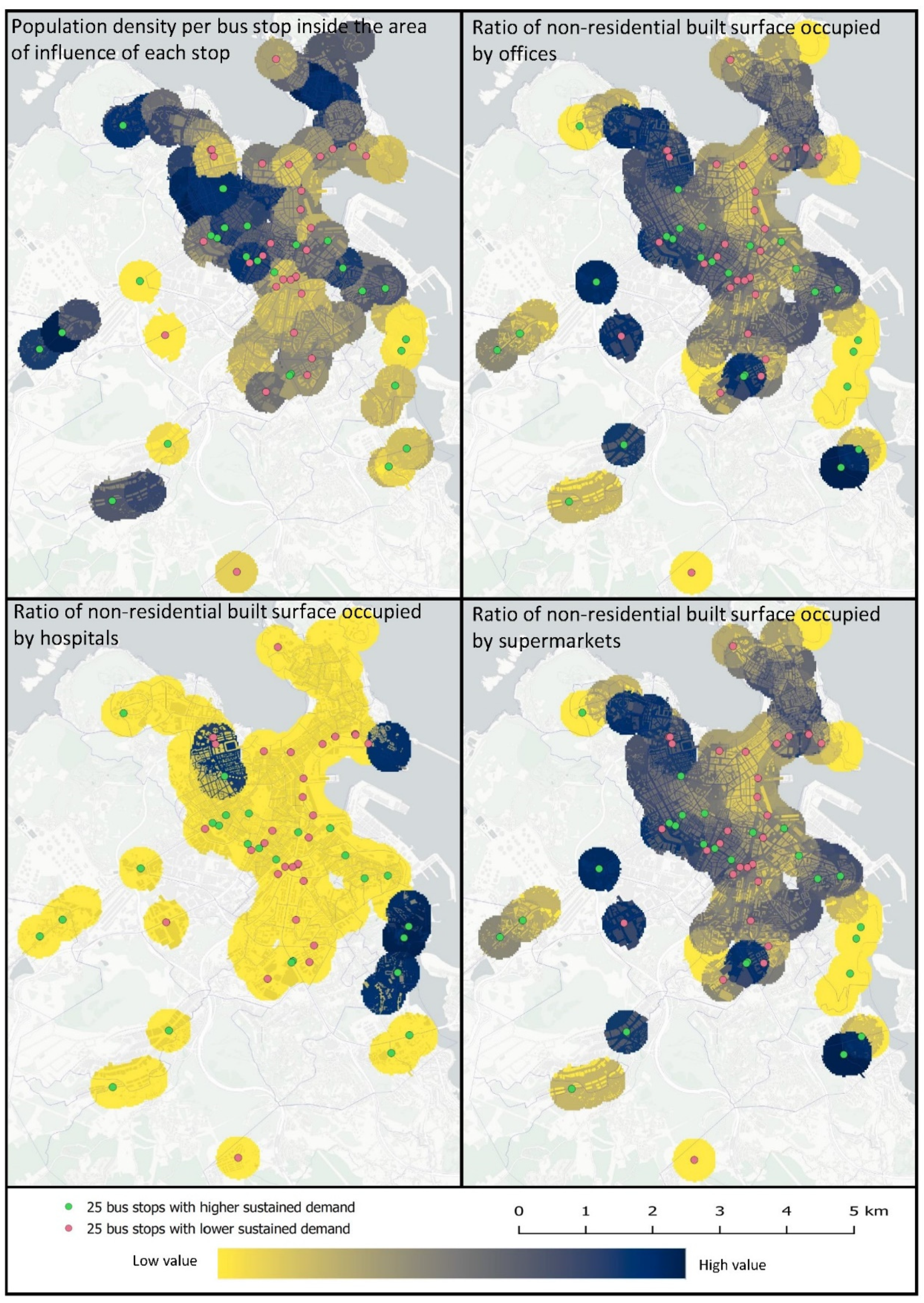
| Pop_dens_stop (1000 inh/km2/bus stop) | Population density (thousands of inhabitants (inh) per square kilometre) per bus stop inside the area of influence of each stop. | 2.9512 | 1.6254 |
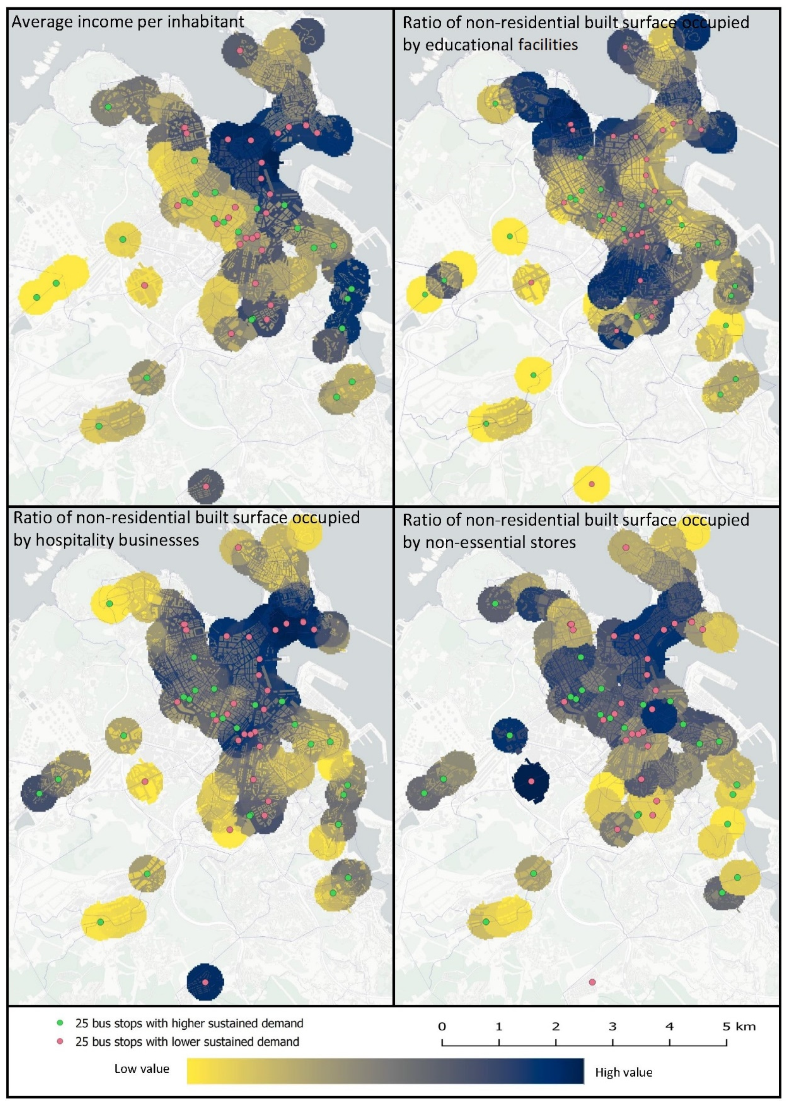
| Ave_income_inh (1000 €/inh) | Average income in thousands of EUR per inhabitant. | 14.2676 | 3.5671 |
| Surf_Educat | Ratio of non-residential built surface occupied by educational facilities. | 0.0152 | 0.0179 |
| Surf_non_ess | Ratio of non-residential built surface occupied by non-essential stores. | 0.0486 | 0.0301 |
| Surf_superm | Ratio of non-residential built surface occupied by supermarkets. | 0.0079 | 0.0114 |
| Surf_office | Ratio of non-residential built surface occupied by offices. | 0.0368 | 0.0325 |
| Surf_hospit | Ratio of non-residential built surface occupied by hospitals. | 0.0126 | 0.0076 |
| Surf_hos_buss | Ratio of non-residential built surface occupied by hospitality businesses. | 0.0119 | 0.0655 |
| Period: Severer Lockdown (28 March–9 April) | ||||
|---|---|---|---|---|
| Dependent Variable: Ratio of Bus Demand in 2020 to 2017–2019 Mean | ||||
| Coefficient | Standard Error | SC | ||
| Const | 0.1529 * | 0.019 | ||
| Pop_dens_stop | 0.0057 * | 0.002 | 0.1802 * | |
| Ave_income_inh | −0.0032 * | 0.001 | −0.2215 * | |
| Surf_Educat | −0.5318 * | 0.198 | −0.1860 * | |
| Surf_non_ess | −0.4496 * | 0.128 | −0.2638 * | |
| Surf_superm | 0.8972 * | 0.309 | 0.1999 * | |
| Surf_office | 0.3893 * | 0.161 | 0.2470 * | |
| Surf_hos_buss | −1.1703 * | 0.522 | −0.1730 * | |
| Surf_hospit | 0.3284 * | 0.059 | 0.4194 * | |
| N | 161 | |||
| R2 | 0.359 | |||
| Adjusted R2 | 0.325 | |||
| Period | February | 1–12 March | 13–14 March | Lockdown (15–27 March) | Severer Lockdown (28 March–9 April) | Lockdown (10 April–3 May) | Phase 0 (4–10 May) | Phase 1 (11–24 May) | Phase 2 (25 May–7 June) | Phase 3 (8–14 June) | New Normal (15–30 June) |
|---|---|---|---|---|---|---|---|---|---|---|---|
| Variable (Coef/SC) | Reopening Process | ||||||||||
| Const | 1.0962 * | 1.0834 * | 0.6672 * | 0.2331 * | 0.1529 * | 0.1837 * | 0.2028 * | 0.2635 * | 0.4717 * | 0.5167 * | 0.5765 * |
| Pop_dens_stop | 0.0036 | −0.0075 | 0.0066 | 0.0047 | 0.0057 * | 0.0078 * | 0.0092 * | 0.0143 * | 0.0048 | 0.0073 | 0.0071 |
| 0.0321 | −0.0656 | 0.0579 | 0.0850 | 0.1802 * | 0.2150 * | 0.2141 * | 0.2984 * | 0.0846 | 0.1309 | 0.1218 | |
| Ave_income_inh | −0.0006 | −0.0005 | −0.0113 * | −0.0053 * | −0.0032 * | −0.0046 * | −0.0036 | −0.0040 | −0.0062 * | −0.0025 | −0.0014 |
| −0.0111 | −0.0104 | −0.2156 * | −0.2128 * | −0.2215 * | −0.2818 * | −0.1833 | −0.1839 | −0.2399 * | −0.0989 | −0.0512 | |
| Surf_Educat | 0.3597 | −0.2973 | −1.4459 * | −0.9668 * | −0.5318 * | −0.6001 * | −0.7261 * | −0.8008 * | −1.3195 * | −1.0310 * | −0.8294 |
| 0.0350 | −0.0286 | −0.1392 * | −0.1940 * | −0.1860 * | −0.1833 * | −0.1859 * | −0.1840 * | −0.2560 * | −0.2053 * | −0.1572 | |
| Surf_non_ess | −0.5641 | −0.6375 | −0.1592 | −0.6339 * | −0.4496 * | −0.4898 * | −0.6372 * | −0.7989 * | 0.0861 | 0.1440 | −0.1034 |
| −0.0920 | −0.1030 | −0.0257 | −0.2135 * | −0.2638 * | −0.2510 * | −0.2738 * | −0.3080 * | 0.0280 | 0.0481 | −0.0329 | |
| Surf_superm | 0.8353 | 0.9113 | 1.4214 | 1.2946 * | 0.8972 * | 1.0646 * | 1.5885 * | 1.0982 * | 0.6605 | 0.3130 | 0.9035 |
| 0.0518 | 0.0559 | 0.0872 | 0.1655 * | 0.1999 * | 0.2072 * | 0.2592 * | 0.1608 * | 0.0816 | 0.0397 | 0.1091 | |
| Surf_office | −0.2832 | −0.0191 | 0.7006 | 0.6318 * | 0.3893 * | 0.4028 * | 0.2738 | 0.4540 | −0.0692 | −0.3177 | −0.1762 |
| −0.0500 | −0.0033 | 0.1224 | 0.2301 * | 0.2470 * | 0.2233 * | 0.1272 | 0.1893 | −0.0244 | −0.1148 | −0.0606 | |
| Surf_hos_buss | 2.4039 | 0.0088 | 1.0065 | −1.3742 | −1.1703 * | −0.7288 | −0.0851 | 1.2395 | −0.1763 | −0.3118 | −0.1325 |
| 0.0988 | 0.0004 | 0.0410 | −0.1166 | −0.1730 * | −0.0941 | −0.0092 | 0.1204 | −0.0145 | −0.0262 | −0.0106 | |
| Surf_hospit | 0.2780 | 0.1788 | 0.2838 | 0.4868 * | 0.3284 * | 0.3350 * | 0.2815 * | 0.2558 * | 0.2040 | 0.1994 | 0.1308 |
| 0.0987 | 0.0629 | 0.0998 | 0.3568 * | 0.4194 * | 0.3737 * | 0.2632 * | 0.2147 * | 0.1446 | 0.1450 | 0.0905 | |
| R-squared | 0.0275 | 0.0249 | 0.1117 | 0.2544 | 0.3592 | 0.3226 | 0.2539 | 0.2104 | 0.1730 | 0.1308 | 0.0767 |
| Adj. R-squared | −0.0236 | −0.0264 | 0.0649 | 0.2152 | 0.3255 | 0.2869 | 0.2146 | 0.1688 | 0.1295 | 0.0850 | 0.0281 |
| Standard Error | 0.1865 | 0.1887 | 0.1370 | 0.0791 | 0.0421 | 0.0496 | 0.0620 | 0.0711 | 0.0862 | 0.0861 | 0.0933 |
Publisher’s Note: MDPI stays neutral with regard to jurisdictional claims in published maps and institutional affiliations. |
© 2022 by the authors. Licensee MDPI, Basel, Switzerland. This article is an open access article distributed under the terms and conditions of the Creative Commons Attribution (CC BY) license (https://creativecommons.org/licenses/by/4.0/).
Share and Cite
Montero-Lamas, Y.; Orro, A.; Novales, M.; Varela-García, F.-A. Analysis of the Relationship between the Characteristics of the Areas of Influence of Bus Stops and the Decrease in Ridership during COVID-19 Lockdowns. Sustainability 2022, 14, 4248. https://0-doi-org.brum.beds.ac.uk/10.3390/su14074248
Montero-Lamas Y, Orro A, Novales M, Varela-García F-A. Analysis of the Relationship between the Characteristics of the Areas of Influence of Bus Stops and the Decrease in Ridership during COVID-19 Lockdowns. Sustainability. 2022; 14(7):4248. https://0-doi-org.brum.beds.ac.uk/10.3390/su14074248
Chicago/Turabian StyleMontero-Lamas, Yaiza, Alfonso Orro, Margarita Novales, and Francisco-Alberto Varela-García. 2022. "Analysis of the Relationship between the Characteristics of the Areas of Influence of Bus Stops and the Decrease in Ridership during COVID-19 Lockdowns" Sustainability 14, no. 7: 4248. https://0-doi-org.brum.beds.ac.uk/10.3390/su14074248