1. Introduction
1.1. Motivation and Background
Power systems are developing in the direction of increasing the proportion of renewable energy power generation and forming a low-carbon energy supply system [
1]. At the same time, with the popularization of a large number of flexible loads, represented by electric vehicles (EV), the double-sided problem of the supply and demand of power systems has become increasingly prominent. The increasing demand for energy required to charge EVs is beginning to pose a growing challenge to the power grid [
2]. The traditional coordinated control method of power following load has been unable to meet the development needs of the power grid [
3]. As an important part of the power system, EVs play an increasingly important role in ensuring the balance of the supply and demand of the power system. On the one hand, the charging behavior of the EVs is transferable and interruptible. On the other hand, as a decentralized energy storage device, EVs can use vehicle-to-grid (V2G) technology as a flexible scheduling resource to rationally adjust their charge and discharge behavior [
4,
5]. However, due to a combination of factors, such as the lack of EV charging infrastructure, high vehicle battery costs, and deficiencies in relevant laws and regulations, the development scale of EVs in different countries and regions varies greatly. Scholars have carried out research on promoting EV development in various aspects, including the location planning of charging stations, the investigation of EV purchase intentions, and the improvement of EV technology [
6,
7]. This paper focuses on the research surrounding the key issues of EVs participating in demand response (DR).
The prerequisite for EVs to participate in DR is that the DR regulation strategy and corresponding DR potential must be accurately analyzed and evaluated. The day-ahead DR time-varying potential evaluation is the basis for the selection of target consumers, and the basis of day-ahead demand-side resource optimization scheduling [
8,
9]. Accurate evaluation of DR potential can better promote the development of DR. The DR potential of EVs is directly determined by the state of charge (SOC) of the EVs. Due to the randomness of residential consumers’ travel and charging behavior, the SOC of EVs is random in time and space. How to accurately establish a travel model for EVs, and calculate the change in SOC with the corresponding time and space, is the basis for DR potential evaluation [
10,
11]. In addition, considering the travel needs of residential consumers, how to reduce the impact of DR on residential consumers in order to achieve non-inductive DR, and achieve the goal of maximizing the charging and discharging potential of EVs, is an urgent problem to be solved [
12,
13].
1.2. Literature Overview
Remarkable work has been conducted with respect to DR potential evaluation of EVs. Some of this research is on the construction of the spatiotemporal activity model of EVs. The authors in [
10] proposed a method to analyze charging demand, and calculated the charging demands of functional regions based on stochastic simulation of the trip chain. In [
12], the authors built a travel activity model for EVs, and obtained the key parameters of the model based on actual data fitting. Then, the DR potential of the EVs delayed charging was calculated. The above authors all considered and analyzed the time and space activity characteristics of EVs. On this basis, the authors in [
13] further considered the influence of peoples’ social attributes on their travel patterns, which improved the accuracy of the charging load forecast model. However, the key parameters of the spatial and temporal activity model were all fitted through existing or improved probability distributions. The fitting results had limitations and poor robustness. Alternatively, research has also been conducted on the calculation of the DR potential of EVs. In [
14], the authors presented a composite methodology that considers the dynamic road network information and fuzzy user participation for obtaining spatiotemporal projections of DR potential from EVs. Based on historical charging data, the authors in [
15] used a BP neural network to construct a schedulable DR potential prediction model. Three factors, including the remaining dwell time, remaining SOC, and incentive electricity pricing, were considered to affect the willingness of the EV consumers to participate in DR, which made the potential evaluation results more in line with the actual situation. The authors in [
16] proposed a probabilistic evaluation method of household EVs dispatching potential, considering consumers’ multiple travel needs. Under the implementation of the time-of-use price mechanism, the potential of the EVs to transfer loads was quantified. The authors in [
17] proposed a method for evaluating the charging and discharging scheduling potential of EVs in case of the occasional operation of a power grid, and quantified the impact of incentives on the response level of the EVs.
To sum up, considering the spatiotemporal characteristics of EV travel, there have been certain research results on the quantitative evaluation of potential. In addition, there are the following problems that need to be solved:
The short-term DR potential of EVs is directly related to the vehicle scheduling strategy. Different DR control types and methods have a direct impact on the potential. It is necessary to consider travel needs and willingness to participate, so as to achieve non-inductive DR control and maximize potential.
It is difficult to obtain refined travel data and charging load data of large-scale EVs. How to evaluate the potential of large-scale EVs based on the small sample data in the DR pilot project is an urgent problem to be solved.
Due to the randomness of the time and space of EV travel, and the state changes of vehicles in DR, the DR potential is diverse at different times of day, and the potential during DR also changes with time. Considering the time-varying nature can further improve the accuracy of potential evaluation.
1.3. Contributions
Aiming to fill the above research gaps, this paper proposes a large-scale, day-ahead potential deduction evaluation method based on the small sample data available for EVs, which mainly applies to residential consumers participating in incentive DR projects. This method provides guidance for the day-ahead scheduling of power system operator, the bidding of load aggregator, and the selection of target consumers. The contributions of this paper are summarized as follows:
The travel activity model of large-scale EVs is established. Based on the actual travel data of a sample of residents, the probability distributions of the key parameters in the travel model are obtained by kernel density estimation (KDE) and probability statistical fitting. The fitting results reflect the irregular distribution of variables, with high accuracy and robustness.
Considering the temporal and spatial distribution of the SOC and the travel demand of the EVs, the non-inductive control strategies of three DR modes (peak-cutting, V2G discharge, and valley-filling) are analyzed. The three DR strategies are independent of each other, which maximizes the DR potential while meeting the travel needs of the EVs.
Based on the three DR strategies, the time-varying characteristics of DR are analyzed separately, including the change in potential with the duration of DR and the change at different periods of in a day. Furthermore, the power change index is defined to quantify the DR potential.
The rest of this paper is organized as follows: In
Section 2, a large-scale potential deduction evaluation method based on small sample data is proposed, and the DR potential of the EVs under different strategies are calculated and analyzed. In
Section 3, the time–space activity model and charging behavior modeling of the EV are established, and the probability distributions of the key parameters are fitted. A case study is presented in
Section 4.
Section 5 is a discussion of the results.
Section 6 concludes the paper.
2. DR Potential Evaluation Method of EV
2.1. EV Load Model
The EV model is based on the relationship between the state of charge (SOC) of the battery and the charge and discharge power [
18]. According to the charging and discharging process of the EV, the initial constant power charging and discharging time accounts for most of the total time. Therefore, it is considered that the EV is charged and discharged at a constant power [
19]. The state of charge and charging power of the EV can be approximated using Equation (1):
where
is the SOC of EV
n at time
;
is the SOC of EV
n at time
t;
is the charge or discharge power of EV
n;
is the battery capacity of EV
n;
is the charging or discharging efficiency of EV
n.
The SOC of the EV is mainly determined by travel distance. Assuming that the battery power of the EV decreases at a constant rate during driving, the relationship between the current SOC of the EV and the distance traveled after the last charge is determined using Equation (2):
where
is the SOC of EV
n at time
;
is the SOC of EV
n at time
;
is the travel distance of EV
n;
is the cruising distance of EV
n.
2.2. DR Control Strategy Analysis of EVs
Under the conditions of meeting the travel needs of residential consumers, the charging and discharging times of the EVs can be flexibly adjusted according to the operation characteristics of the power grid. The DR types and potentials of EVs are different under different DR control strategies. These can be divided into three categories: peak-shaving strategy, valley-filling strategy, and V2G discharge strategy.
2.2.1. Peak-Shaving DR Strategy
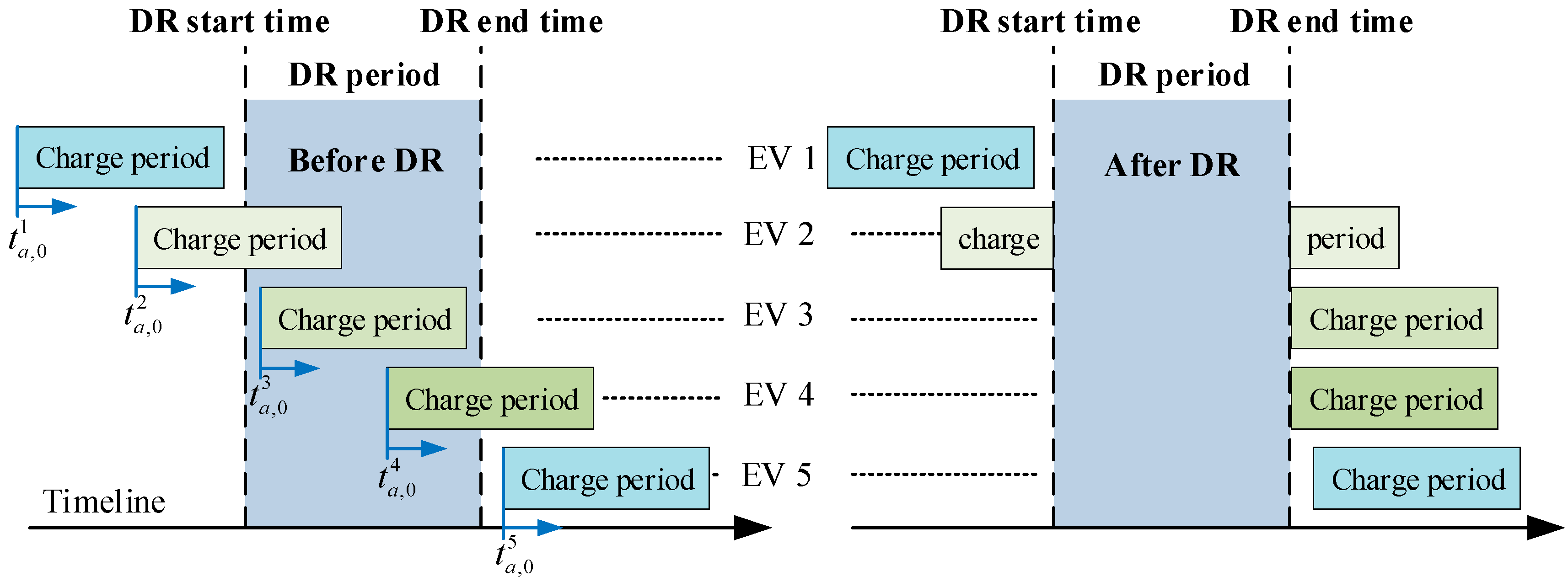
During the DR period, the charging EV reduces the charging time, or stops charging completely, to achieve the purpose of load reduction during this period. The change in the charging time of the EVs before and after DR is shown in
Figure 1. When the EVs are not participating in DR, they start charging immediately after arriving home, at time
. When the EVs participate in DR, the charging times of EVs 2, 3, and 4 are changed. The charging load during the DR period is shifted to after the DR ends. Since EV 1 and EV 5 do not perform charging during the DR period, their peak-shaving potentials are 0. It is worth noting that if an EV participates in DR and affects future travel demand, the EV does not participate in this DR event.
2.2.2. Valley-Filling DR Strategy
For valley-filling DR, during the DR period, the EVs are charged to the maximum extent, i.e., until the SOC reaches the upper limit. The charging changes of five types of EVs before and after participating in DR are shown in
Figure 2. EV 1 and EV 2 do not charge immediately after returning home at time
, and delay charging until the DR period, thereby absorbing the power generation load of the power grid. The times when EVs 3, 4, and 5 arrive home are after the DR start time, and their charging behaviors do not change.
2.2.3. V2G Discharge Strategy
For the V2G discharge DR, the remaining SOC of the participating EVs after arriving home is required to meet the next day’s trip, and must be greater than the expected minimum SOC. During the DR period, this type of EV maximizes the reverse discharge to the grid as much as possible, and recharges it to the initial SOC after the DR ends. The V2G DR can relieve the power supply pressure on the source side, and its effect is the same as that of the peak-shaving DR. In addition, the EVs that meet the V2G conditions have no charging demand after arriving home, and they do not conflict with the EVs participating in peak-shaving DR. Therefore, the two DR control strategies can be implemented simultaneously to maximize load peak shaving.
2.3. DR Potential Evaluation of EVs
The power change during the DR period can be calculated by subtracting the power after DR from the power before DR. Based on the battery charging and discharging physical model, the peak-shaving and valley-filling power of each EV during DR can be calculated. Since the states of the EVs connected to the power grid directly affect the category of potential, the charge and discharge state quantity,
, is introduced. The generalized function of the time-varying potential of the EV is defined as shown in Equation (3):
where
is the state of the EV connected to the power grid (1 means charging, −1 means discharging, and 0 means neither charging nor discharging);
t is the duration of DR;
is the charge and discharge power of the EV;
is the charge and discharge efficiency;
is the battery capacity of the EV.
Based on the potential generalized function , the premise of predicting the potential of the EV is to determine the specific values of each input variable of the function. For , , and , their values depend on battery equipment parameters, which can be directly obtained through questionnaire survey or identified through charging load mining. The SOC of the EV directly determines the response potential, and its value depends on the daily travel behavior of the resident consumers. Due to the randomness and variability of travel behavior, the calculation of SOC is relatively complicated. It is necessary to build a travel time–space activity model based on the historical travel data of the EV. Based on the travel activity model, the SOC of the EV can be predicted and calculated. The value of depends on the SOC of the EV and the resident consumers’ preference for charging and discharging behavior. In addition, determines the type of DR that the EV can participate in. Therefore, a resident consumers’ charging and discharging behavior model needs to be established in order to calculate .
Since EVs are not widely used at present, it is difficult to obtain refined travel data and charging and discharging data of large-scale EVs. It is difficult to directly obtain the parameters of each EV potential function in a large area. This paper proposes a large-scale potential deduction evaluation method based on the small sample data available for EVs, as shown in
Figure 3. First, based on the multivariate historical small sample data of EVs, an EV physical model, an EV spatiotemporal activity model, and a charging behavior model are constructed, respectively. On this basis, a comprehensive model of the EVs’ charging and discharging loads is constructed, and Monte Carlo (MC) simulation is used to predict and calculate the EVs’ charging loads. Finally, considering the various factors influencing the potential, combined with the different states and control strategies of EVs, one can calculate and analyze peak-shaving potential, valley-filling potential, and V2G discharge potential.
3. Model of EV Behavior
EV behavior includes travel behavior and the charging and discharging behavior of resident consumers. The two together determine the SOC and network access state of the EV after it arrives home.
3.1. Time–Space Activity Model of EVs
3.1.1. Travel Chain Model
Residential consumers’ EV charging demand is closely related to their travel behavior; thus, the accurate establishment of the consumers’ travel model is the basis for analyzing the charging load of the EVs. Based on the residential travel chain, this paper constructs a dynamic time–space model of consumer travel [
10,
13]. The travel chain of the EV is defined as follows: the EV starts from home, complies with the residents’ travel activities, reaches different travel destinations in a certain time sequence, and finally returns home. The entire travel chain contains a large amount of interrelated travel information in time and space, as shown in
Figure 4.
The time and space eigenvalues of EV
n are extracted. Time characteristic values include time
when arriving at location
i, time
when leaving location
i, travel time of the
ith trip
, and parking time
at location
i. The first travel time is
. Taking
,
, and
as input variables, the arrival time
and departure time
can be calculated using Equations (4) and (5).
Spatial characteristic values include destination type for the ith trip, travel distance for the ith trip, total length of a day’s travel chain , and space transition probability . The value of is a set at D = {H,W,O}, where H, W, and O indicate home, work place, and other locations, respectively. refers to the probability of the EV traveling to the destination for the ith trip from the location .
It has been found that the above characteristic values, once determined, can fully reflect the daily travel behavior of residential consumers [
20]. In this paper, MC simulation is used to generate each characteristic value. The basis of MC simulation is to obtain the probability distribution of each characteristic value [
21,
22]. Existing research mainly uses the conventional form of probability distribution to fit, such as normal distribution, etc. The fitting results are acceptable under certain conditions. However, for statistical data exhibiting distribution characteristics sufficiently different from the common distribution form, such as in a multimodal distribution, fitting is no longer applicable. To this end, this paper conducts a probability analysis on the characteristic values of residential consumers’ actual travel, uses KDE to fit the actual distribution of the characteristic values, and then obtains the probability density curve of each characteristic value.
3.1.2. Probability Distribution of Characteristic Values
KDE is used to estimate unknown density functions in probability theory, and is a non-parametric testing method [
23,
24].
,
,…
are independent and identically distributed
k sample points, and
is the probability density function. The kernel density estimation of
is presented as Equation (6):
where
k is the sample size;
h is the bandwidth;
K is the kernel function. The above parameters satisfy Equations (7)–(9).
This article chooses a Gaussian kernel function, as shown in Equation (10).
Based on the actual sample data for travel, using the method of KDE, the probability density functions of the three key characteristic values,
,
, and
can be obtained. Then, the specific value of the travel chain can be obtained by simulation sampling. For the calculation of the characteristic value
, the travel time and the travel distance are directly related to the speed
. At different time periods,
is different; thus, considering different time periods, the relationship between
and is linearly fitted, as in Equation (11).
Based on Equations (5) and (6), the remaining time is calculated, and a complete time chain can be obtained.
For the spatial characteristic values, the probability density function of can also be obtained using KDE. For the travel chain length , the frequency of the travel chain length of all EVs is calculated. By approximating the probability by frequency, different travel chain lengths and their corresponding probability values are obtained. It is worth noting that the restriction on the length of the travel chain is added to prevent the situation where the travel chain of the EV is too long when the travel path of the EV is simulated, and it is unknown when the travel chain should be ended. This causes the simulation results to deviate greatly from reality. Therefore, at a location before the end of the travel chain, the EV’s last travel destination is set as home.
For the spatial transition probability
, the transition probabilities of different starting points and corresponding end points are different. At the same time, the transition probabilities are also different for different time periods in a day. Therefore, the spatial transition probability is determined by the time period and the current location [
25].
is discretized at a certain time interval, and a three-dimensional matrix of the EV, with a scale of
M × 3 × 3, can be obtained. This matrix is defined as the travel location transition probability matrix.
M is the number of time intervals after discretization, and there are three types of travel locations, H, W and O. Taking a cross-section at any time interval
, a 3 × 3 two-dimensional matrix is obtained, as shown in Equation (12):
where
is the transition probability of the vehicle from H to W during period
. The sum of any rows of the matrix
is 1, which means that the sum of the probabilities for the EV to select each destination type is 1.
3.2. Charging and Discharging Behavior Model of EVs
Considering that after the EVs leave home, they will charge in other areas outside the home, which will affect the charging load at home to a certain extent [
26]. In addition, the charging and discharging behaviors of the EVs also affects the grid-connected state
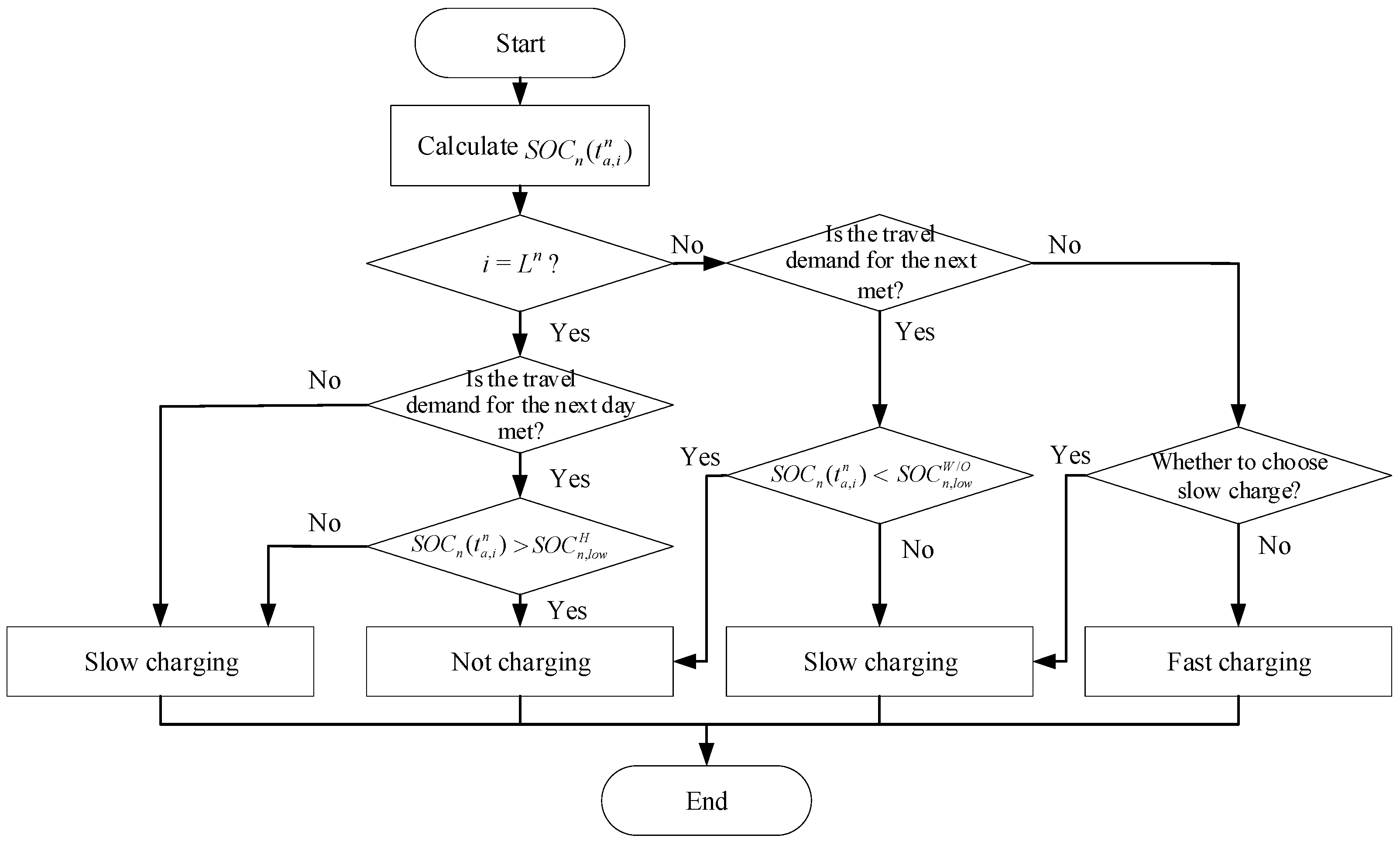
S of the EVs. In this section, the EV charging judgment model is constructed based on EV historical charging habits, as shown in
Figure 5. Combined with the time–space activity model, it further calculates the SOC changes of the EVs over the course of a day.
The charging power is set to two types: slow charging and fast charging. Under normal circumstances, slow charging is the main method, whereas fast charging is selected in emergencies [
27]. Residential consumers only charge their EVs during parking hours. If the parking time is over and the battery is not fully charged, the charging is also stopped.
The following are the charging conditions:
After the EV arrives at the parking location, if the remaining power is not enough to support the next drive, it must be charged. There are two charging powers to choose from: slow charge or fast charge. Slow charge is preferred; however, if in the slow charge mode the supplementary power is still not enough to support the next drive, then the fast charge mode is adopted.
If the remaining power is sufficient for the next drive, slow charging or no charging can be selected. Considering factors such as battery safety and remaining power anxiety, every residential consumer has his own minimum acceptable SOC. is the minimum acceptable SOC at home, and is the minimum acceptable SOC at the work place or other location. If the remaining SOC of the battery is lower than the minimum SOC, the slow charge is still selected for charging.
Combining the travel chain model of the EVs and the simulation model of the charging behavior of the residents, the one-day change curve of the SOCs of the EVs and the charging load curve in the residential area can be obtained.
3.3. Travel Chain and Load Simulation of EVs
Based on the time–space activity model and the charging behavior model of EVs, MC simulations are used to simulate and predict travel data and charging load data for large-scale EVs [
28]. The travel simulation flow chart of
N EVs is shown in
Figure 6.
Taking the EV n as an example, the specific simulation process is as follows:
Enter the probability distribution of the characteristic values of the travel chain , , , ,.
Sampling to obtain the total length of the travel chain.
Sampling to obtain the time of the first trip of the day.
Sampling to obtain the travel destination. According to the current location type and travel time, select the corresponding spatial transition probability and conduct sampling.
Sampling to obtain the driving distance. Considering the starting point and end point of the drive, select the corresponding probability distribution for sampling.
Calculate travel time. Considering different driving periods, calculate the corresponding driving time based on Equation (11). Calculate the arrival time at the destination based on Equation (4).
Sampling to obtain the parking time. Calculate the next travel time based on Equation (5).
Return to step (4) and re-enter the loop until the travel chain length meets the requirements.
Combining the travel chain model of the EVs and the simulation model of the charging behavior of the residents, the one-day change curve of the SOC of the EVs and the charging load curve in the residential area can be obtained.
4. Case Study
The DR service in this article is aimed at the coastal cities in southeastern China. The DR is in the form of an invitation one day in advance, and consumers can acquire a certain incentive compensation after participating in the DR. During DR, large industrial and commercial users directly participate in the response, while distributed flexible loads, such as those of electric vehicles, participate in grid load regulation centrally through load aggregators. China’s demand response development over the past five years is shown in
Table 1. Various regions have carried out relevant DR pilot projects, which are generally in their infancy [
29,
30]. For EV loads, it is currently difficult to directly obtain detailed travel data of EVs in most areas of China.
Therefore, in the case study, data come from the travel database of the U.S. National Household Travel Survey (NHTS). The NHTS data are the main source of information on daily travel linked to individual personal and household characteristics, socio-economic characteristics, vehicle ownership, and vehicle attributes. Since there are few travel records for EVs, this paper selects the travel data of all types of vehicles, including fuel vehicles, for analysis. In the database, travel information of each trip for each vehicle during a day is recorded, including start and end time, driving time, driving distance, and parking time [
31]. The NHTS data were collected between April 2016 and May 2017, and are the nation’s source of information regarding travel by U.S. residents in all 50 states and the District of Columbia. On the basis of the original data, after cleaning and processing, the recorded data of 678,000 trips made by 101,005 households were finally selected. Among them, there are 173,296 complete travel chain data, where the vehicle departed from home and finally returned home. The daily travel records of 100 vehicles are shown in
Figure 7. The vehicle sequences are sorted in the order of initial time of leaving home. It can be seen that there are differences in the travel behaviors of different vehicles. During the travel process, the corresponding times and travel distances are fully recorded.
4.1. Calculation of Characteristic Values in the Travel Chain
For first travel time, with travel distance and parking time as the characteristic values, KDE in
Section 3.1 is used to calculate the probability density curve, which can accurately reflect the true distribution of the actual data. The results show that most EVs depart from home for the first time between 7:00 and 9:00, and the travel distance of most EVs is concentrated around 10 km. For the parking time, considering the impact of different time periods and locations on the length of parking, one day is divided into 24 h. In each time period, the probability density curve of the parking time of the EVs at different locations is calculated.
For travel time, considering the influence of time periods, a day is divided into 24 time periods, each of which is one hour. In each period, the relationship between travel time and travel distance is fitted separately.
For space transition probability, considering the influence of different starting points and end points, the probability distributions of four time periods, 7:00 to 8:00, 11:00 to 12:00, 15:00 to 16:00, and 19:00 to 20:00, are shown in
Figure 8.
For travel chain length, the corresponding probabilities of different travel chain lengths are counted and calculated. Of these, 46% of EVs have a travel chain length of 2, which may mean that the EVs travel from home to work and then back home.
4.2. Verification of Simulation Results of the Travel Chain
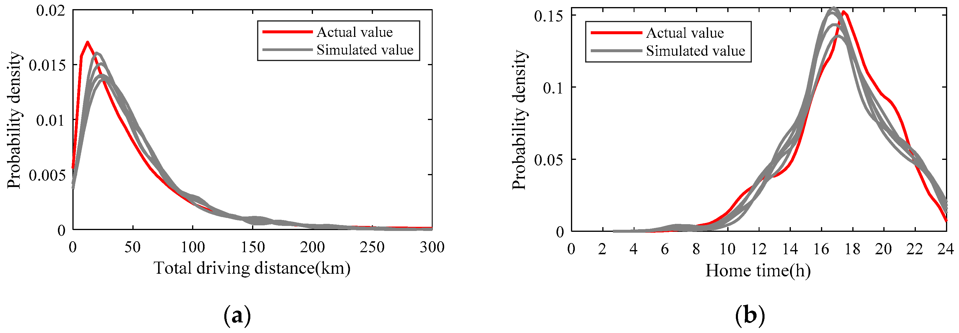
Using the above probability distribution as the input variable, the travel situations of 1000 EVs were simulated based on the simulation flow in
Figure 6. In order to further verify the validity of the simulation results of the EV travel, they are compared with the actual NHTS data. During a one-day trip, parameters such as the travel chain length, first travel time, travel distance, time to each destination, and parking time of each EV can be directly obtained through probability sampling. These parameter probability distribution laws are calculated based on actual data, so it is meaningless to compare the simulation results with actual data. However, the total daily driving distance and home time of an EV are indirectly calculated based on the data for each trip, so the values of these two parameters have no direct correlation with the actual data. The statistical results of their probability distribution are compared with the actual data, which can reflect the difference between the simulation results and the actual values. In addition, the total daily driving distance is directly related to the SOC after the EV arrives home, and the home time is related to the time parameter of the charging load. Accurate simulation of the total daily driving distance and home time can further improve the charging load prediction accuracy and potential assessment accuracy of EV groups. Therefore, the total daily driving distance and home time are finally selected as the verification parameters for the comparison between the simulated value and the actual value.
The probability distribution results of the simulation value obtained indirectly by calculation, and the actual value obtained directly from the database, are shown in
Figure 9. In order to fully verify the validity of the simulation results, the EV group is simulated five times, and the simulation errors of each time are calculated separately. The root mean square error (RMSE) and correlation coefficient (r) are used to measure the accuracy of the simulation. The results are shown in
Table 2. It can be seen that the simulated driving law is closer to the actual characteristics, which verifies the validity of the travel chain model. The average RMSE and correlation coefficient of travel distance are, respectively, 0.0014 and 0.9522. The average RMSE and correlation coefficient of end time are, respectively, 0.0112 and 0.9705.
4.3. Simulation Results of Charge Load
The battery parameter information of the EV can be obtained by counting the EV models of the residential area. In this paper, according to the EV models on the market, the EV battery parameters are set to the following five types. The battery capacity is set to 57, 19, 60, 85, and 28 kWh. The corresponding power consumption per kilometer is set to 0.195, 0.129, 0.154, 0.193, and 0.166 kWh. The battery parameters of these five types of EVs each account for 20%.
The slow charge power and fast charge power are 3.5 kW and 12 kW, respectively. Considering the safety factors of battery charging and discharging, the upper and lower limits of SOC are set to 0.9 and 0.1. The minimum acceptable SOC is set to obey a normal distribution. obeys the normal distribution N(0.6, 0.052) and obeys N(0.3, 0.052).
The load curve is simulated continuously for multiple days, and the middle day is taken for analysis to reduce the influence of parameter initialization. The charging load of large-scale EVs for weekdays and weekends are shown in
Figure 10. Due to the randomness of charging behavior, the EV charging load varies on different days. There is a positive correlation between the total charging load of the vehicle and the time of leaving or arriving home. Compared with weekdays, the vehicle leaves and arrives at a later time on weekends, which results in a certain degree of delay in the charging load on weekends. Taking a working day as an example for a specific analysis, the charging load reaches its peak between 18:00 and 24:00 in the evening, and is at a low point between 8:00 and 14:00 during the day. This is due to the travel behavior of residents leaving home at around 8:00 in the morning and returning home at around 18:00 in the evening.
4.4. DR Potential Calculation Results
Based on the strategy of the EVs participating in DR outlined in
Section 2.3, DR potential under the three strategies (peak-shaving type, valley-filling type, and V2G discharge type) are calculated and analyzed respectively.
4.4.1. Peak-Shaving DR Potential
On the basis of EV charging load, a certain period of time is considered to carry out DR, and the time-varying potential of DR in this period is calculated. The start time of DR is set at 20:00 and the end time is 22:00. During this period, peak-shaving DR is performed; the loads of the EVs before and after DR are shown in the
Figure 11. During this DR period, the load peak-shaving potential averaged 726 kW, which is 82.97% of the average EV load in this period.
The DR potential of the EVs varies at different times of the day. Considering this time variability, different DR events are simulated for one day, and the corresponding DR potential is calculated. Different DR events, and the corresponding start and end time settings, are shown in the
Table 3. The duration of all DR events is 2 h. It is worth noting that each DR event in the table is independent of each other; that is, DR is only carried out at one time period in a day, and is therefore not carried out at all time periods.
For each DR period, the potential of peak-shaving type is shown in
Figure 12. It can be seen that the DR potential is constantly changing during the DR period, and the direction of change is positively correlated with the slope of the charging load curve in
Figure 10. This is because the change in the number of the EVs in the residential area directly determines the change in the continuous potential of DR.
4.4.2. Valley-Filling DR Potential
The analysis method of the valley-filling type DR potential is the same as that of the peak-shaving type. The potential of valley-filling DR is calculated separately for different time periods of one day, the calculation results are shown in
Figure 13. It can be observed that the DR potential of the valley-filling type is at a higher value at night. This is of great significance for absorbing wind power generation and alleviating the anti-peak-shaving phenomenon of wind power generation. In addition, according to the analysis of the trends of the potential changes at different periods of the day, it can be demonstrated that the potential decreases gradually with increasing duration before 12:00, and the opposite is true after 12:00.
4.4.3. V2G Discharge DR Potential
The DR potential of the V2G discharge type is shown in
Figure 14. The valley-filling potential is also time-varying, and its degree of variation is lower than that of the peak-shaving type. This is because the number of the EVs that can participate in valley-filling DR is large. It is less affected by leaving and arriving EVs, and can be charged stably to complete power consumption during the DR period. For the EVs that can participate in V2G discharge DR, the SOC of the battery is sufficient. They will not conflict with the EVs that participate in peak-shaving type. Therefore, the power supply pressure during peak hours of the power grid can be further relieved.
4.4.4. Comparative Analysis of Three Types of Potential
Due to the time-varying potential in the DR period, the quantitative indicators of DR potential are set, which are the maximum response, minimum response, and average response during the DR period. Under three different DR strategies, the calculation results of the maximum response, minimum response, and average response are shown in
Figure 15. Scenario 1 represents the peak-shaving type DR, and the EVs suspend charging during the DR period. Scenario 2 represents the V2G discharge type DR, and the EVs discharge to the grid in the reverse direction during the DR period. Scenario 3 represents the valley-filled DR, and the EVs are charged to the greatest extent during the DR period.
It can be found that the DR potential of the EVs is greater between 18:00 and 4:00 the next day. This is because most EVs are at home during this period. For the peak-shaving type and the V2G discharge type DR under the peak-shaving potential, it can be seen that the potential of the V2G discharge type DR is three to five times that of the peak-shaving type. Therefore, a large number of potential resources can be tapped under the V2G characteristics of the EVs.
4.4.5. Interaction Analysis of Potential in Different Periods
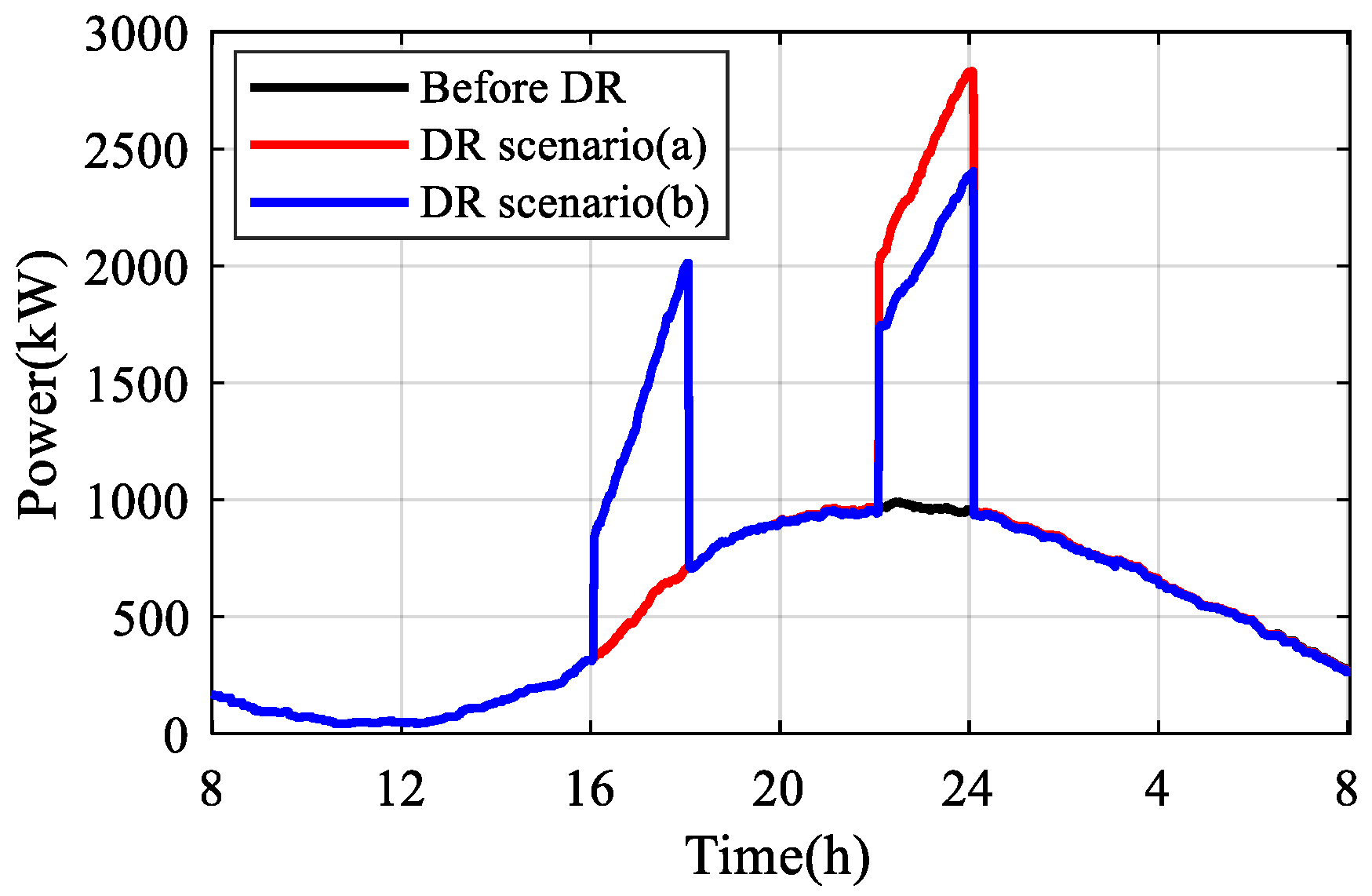
Under the above three DR strategies, the calculation of DR potential at different times of the day is independent of each other. This only satisfies the analysis needs of only one DR event per day. In fact, the EVs may participate in DR in multiple periods of the day, so the potential estimation needs to consider the impact of scheduling results of the EVs in historical periods.
Figure 16 shows the load curve changes after carrying out DR twice in one day. In scenario (a), DR is performed only once between 22:00 and 24:00. The maximum, minimum, and average values of the DR potential for this period are 1876 kW, 1046 kW, and 1491 kW, respectively. In scenario (b), DR is carried out twice in a row from 16:00 to 18:00 and 22:00 to 24:00. It can be observed that the valley-filling potential decreases during the second DR due to the influence of the first DR event. The maximum, minimum, and average values of the DR potential for the second period are 1456 kW, 766.5 kW, and 1096 kW, respectively, which are reduced by 22.39%, 26.72%, and 26.49% compared to scenario (a). The impact of such historical DR events on the evaluation of future load potential needs to be considered in multiple DR scheduling.
5. Discussion
Considering a variety of factors, this paper completes the quantification of the time-varying potential of an EV group based on a small sample of travel data. The results show that there are obvious differences in the potential under different time periods and control strategies.
In residential areas, the charging load curve of electric vehicles is affected by the daily travel behavior of the residents, as shown in
Figure 10. The load is at a trough around 11:00 and peaked at around 23:00, which is consistent with the research results of [
10,
12]. On this basis, the DR potential of the EV is calculated at different time periods. The variation trends in potential within a day are consistent with the charging loads, and the fundamental reason for this is that the spatial location of EVs is constantly changing, and the number of vehicles in the residential area varies among different time periods. In non-residential areas, the trend of potential changes is reversed, as shown in the results of [
14].
In addition, this paper calculates and compares the DR potential under different control strategies, as well as the time-varying potential during the DR process. The overall potential of peak-shaving DR is the lowest, with reference to the average value index, the maximum load can be reduced by 0.75 MW in one day, and the lowest value is 0.08 MW. The valley-filling DR has the greatest potential overall, with a maximum load reduction of 1.75 MW and a minimum of 0.4 MW in one day. The V2G discharge potential of EVs can further complement the peak-shaving potential. The maximum peak-shaving potential and valley-filling potential of 1000 EVs are 2.7 MW and 2.1 MW, respectively. In the process of DR, the time-varying potential is also more obvious, especially the valley-filling DR. Its trend is related to the number of the EVs that are about to leave or enter residential areas. In addition, this paper preliminarily analyzes the impact of historical DR events on the assessment of future potential. After an EV participates in a certain DR, its state and charging load change, which usually leads to a decrease in the potential value of the same type of DR, and there may be an obvious load rebound phenomenon.
The time-varying potential calculation results of EVs can provide effective guidance for their participation in power system dispatching. There are many types of flexible loads on the demand side, and EVs, as one of them, can preferentially participate in DR during periods of abundant potential, while other flexible loads participate in DR during other periods. This takes full advantage of the time-domain complementarity of heterogeneous flexible loads. The time-varying potential of the DR process needs to be focused on when participating in system frequency modulation. Additionally, the volatility of potential can be reduced by means of grouped round-robin control. Therefore, the research results of this paper can lay a foundation for the development of a normalized demand response.
Some limitations to this study are identified in the following. First, this paper only reports case studies based on NHTS data, and the results of the potential calculations may vary in other regions. The DR potentials of different regions need to be recalculated based on local user travel data. Secondly, a consumers’ willingness to participate directly affects the DR potential. This paper does not deeply consider the participation willingness of different consumers in potential calculation. Third, this paper only analyzes the DR potential of EVs for residential areas. Due to the spatial mobility of EVs, there is also great DR potential to be tapped from commercial buildings, public parking lots, and other locations.
6. Conclusions
In this paper, considering the time and space characteristics and travel needs of EVs, a small-sample-data-driven evaluation method for the evaluation of the time-varying DR potential of EVs in residential areas is proposed. The evaluation method mainly consists of three parts: key parameter fitting of the travel chain model based on KDE, EV charging load simulation based on MC, and the calculation of time-varying potential under three different DR strategies. Based on the actual load data from the NHTS, the accuracy of the evaluation method is verified. The results show the charging load reaches its peak between 18:00 and 24:00, and is at a low point between 8:00 and 14:00. Correspondingly, the variation trend of DR potential of EVs at different periods of the day is the same as that of load. In the process of DR events, the aggregate potential of EVs is time-varying, and the direction of change is positively correlated with the slope of the charging load curve. At different times of the day, the change in DR potential is positively correlated with the charging load. Additionally, the potential of the V2G discharge type DR is three to five times that of the peak-shaving type DR. Therefore, a large number of potential resources can be tapped under the V2G characteristics of EVs. In addition, historical DR events have a direct impact on future load status, which in turn changes the results of previous potential evaluations. Subsequent research will further consider the interaction between EV scheduling control and real-time potential, and the DR recovery control strategy to suppress load rebound, on the basis of this paper.
Author Contributions
Conceptualization, S.D.; methodology, C.X.; software, Z.S.; validation, Y.R.; formal analysis, Z.Z.; investigation, Z.C.; resources, S.D.; data curation, Z.S.; writing—review and editing, S.D.; supervision, W.Y. All authors have read and agreed to the published version of the manuscript.
Funding
This research received no external funding.
Acknowledgments
The authors would like to thank Federal Highway Administration for National Household Travel Survey data in this study. Its website:
https://nhts.ornl.gov/, accessed on 1 March 2021.
Conflicts of Interest
The authors declare no conflict of interest.
Abbreviations
| DR | Demand response | i | Index of trips and locations |
| EV | Electric vehicle | | Charging and discharging efficiency of EV |
| H | Region type–Home | N | Number of EVs |
| KDE | Kernel density estimation | n | Index of EVs |
| MC | Monte Carlo | | Spatial transition probability |
| NHTS | National household travel survey | | Travel chain length probability |
| O | Region type–Other location | | Charge and discharge power |
| RMSE | Root Mean Squared Error | | State of EV connected to the power grid |
| SOC | State of charge | | Minimum SOC for charging at home |
| V2G | Vehicle-to-grid | | Minimum SOC for charging at work or other location |
| W | Region type–Work place | t | Index of times |
| Variables | | | Time when EV n arrives at location i |
| Battery capacity of EV | | Time when EV n leaves location i |
| Cruising distance of EV | | The time for EV n to arrive at location i from location i−1 |
| Time-varying potential of the EV at time t | | Parking time of EV n at location i |
| Distance from location i−1 to location i | | Type of location i |
| DR potential generalized function of EV | | The average speed of the vehicle from location i−1 to location i |
| | | | Distance error from location i−1 to location i |
References
- Li, L.; Lin, J.; Wu, N.; Xie, S.; Meng, C.; Zheng, Y.; Wang, X.; Zhao, Y. Review and outlook on the international renewable energy development. Energy Built Environ. 2022, 3, 139–157. [Google Scholar] [CrossRef]
- Macioszek, E.; Sierpiński, G. Charging Stations for Electric Vehicles—Current Situation in Poland. Transp. Syst. Telemat. (TST) 2020, 124–137. [Google Scholar] [CrossRef]
- Kakran, S.; Chanana, S. Smart operations of smart grids integrated with distributed generation: A review. Renew. Sustain. Energy Rev. 2018, 81, 524–535. [Google Scholar] [CrossRef]
- Zhu, L.; Liu, S.; Tang, L.; Ji, J.; Hang, C. Uncertain response modeling of charge and discharge and day-ahead scheduling strategy of electric vehicle agents. Power Syst. Technol. 2018, 42, 3305–3314. [Google Scholar] [CrossRef]
- Mohammad, A.; Zuhaib, M.; Ashraf, I.; Alsultan, M.; Ahmad, S.; Sarwar, A.; Abdollahian, M. Integration of electric vehicles and energy storage system in home energy management system with home to grid capability. Energies 2021, 14, 8557. [Google Scholar] [CrossRef]
- Ling, Z.; Cherry, C.R.; Wen, Y. Determining the Factors That Influence Electric Vehicle Adoption: A Stated Preference Survey Study in Beijing, China. Sustainability 2021, 13, 11719. [Google Scholar] [CrossRef]
- Macioszek, E. Electric Vehicles—Problems and Issues. Transp. Syst. Theory Pract. (TSTP) 2019, 169–183. [Google Scholar] [CrossRef]
- Chen, S.; Chen, Q.; Xu, Y. Strategic Bidding and Compensation Mechanism for a Load Aggregator with Direct Thermostat Control Capabilities. IEEE Trans. Smart Grid 2018, 9, 2327–2336. [Google Scholar] [CrossRef]
- Qi, N.; Cheng, L.; Xu, H.; Wu, K.; Li, X.; Wang, Y.; Liu, R. Smart meter data-driven evaluation of operational DR potential of residential AC loads. Appl. Energy 2020, 279, 115708. [Google Scholar] [CrossRef]
- Wen, J.; Tao, S.; Xiao, X.; Luo, C.; Liao, K. Analysis on Charging Demand of EV Based on Stochastic Simulation of Trip Chain. Power Syst. Technol. 2015, 6, 1477–1484. [Google Scholar] [CrossRef]
- Chen, L.; Zhang, X.; Figueiredo, A. Summary of Research on Electric Vehicle Charge and Discharge Load Forecast. Autom. Electr. Power Syst. 2019, 43, 177–191. [Google Scholar] [CrossRef]
- Qian, T.; Li, Y.; Guo, X.; Chen, X.; Liu, J.; Mao, W. Calculation of electric vehicle charging power and evaluation of demand response potential based on spatial and temporal activity model. Power Syst. Prot. Control 2018, 46, 127–134. [Google Scholar] [CrossRef]
- Zhang, J.; Yan, J.; Liu, Y.; Zhang, H.; Lv, G. Daily electric vehicle charging load profiles considering demographics of vehicle users. Appl. Energy 2020, 274, 115063. [Google Scholar] [CrossRef]
- Chen, L.; Zhang, Y.; Figueiredo, A. Spatio-Temporal Model for Evaluating Demand Response Potential of Electric Vehicles in Power-Traffic Network. Energies 2019, 12, 1981. [Google Scholar] [CrossRef] [Green Version]
- Zhan, X.; Yang, J.; Han, S.; Zhou, T.; Wu, F.; Liu, S. Two-stage Market Bidding Strategy of Charging Station Considering Schedulable Potential Capacity of Electric Vehicle. Autom. Electr. Power Syst. 2021, 45, 86–96. [Google Scholar] [CrossRef]
- Gan, L.; Chen, X.; Yu, K.; Zheng, J.; Du, W. A Probabilistic Evaluation Method of Household EVs Dispatching Potential Considering Users’ Multiple Travel Needs. IEEE Trans. Ind. Appl. 2020, 56, 5858–5867. [Google Scholar] [CrossRef]
- Wu, F.; Yang, J.; Zhan, X.; Liao, S.; Xu, J. The Online Charging and Discharging Scheduling Potential of Electric Vehicles Considering the Uncertain Responses of Users. IEEE Trans. Power Syst. 2021, 36, 1794–1806. [Google Scholar] [CrossRef]
- Das, S.; Acharjee, P.; Bhattacharya, A. Charging Scheduling of Electric Vehicle Incorporating Grid-to-Vehicle and Vehicle-to-Grid Technology Considering in Smart Grid. IEEE Trans. Ind. Appl. 2021, 57, 1688–1702. [Google Scholar] [CrossRef]
- Wei, Z.; Li, Y.; Cai, L. Electric Vehicle Charging Scheme for a Park-and-Charge System Considering Battery Degradation Costs. IEEE Trans. Intell. Veh. 2018, 3, 361–373. [Google Scholar] [CrossRef]
- Ding, T.; Zeng, Z.; Bai, J.; Qin, B.; Yang, Y.; Shahidehpour, M. Optimal Electric Vehicle Charging Strategy with Markov Decision Process and Reinforcement Learning Technique. IEEE Trans. Ind. Appl. 2020, 56, 5811–5823. [Google Scholar] [CrossRef]
- Iwafune, Y.; Ogimoto, K.; Kobayashi, Y.; Murai, K. Driving Simulator for Electric Vehicles Using the Markov Chain Monte Carlo Method and Evaluation of the Demand Response Effect in Residential Houses. IEEE Access 2020, 8, 47654–47663. [Google Scholar] [CrossRef]
- Zhang, T.; Chen, X.; Zhe, Y.; Zhu, X.; Di, S. A Monte Carlo Simulation Approach to Evaluate Service Capacities of EV Charging and Battery Swapping Stations. IEEE Trans. Ind. Inform. 2018, 14, 3914–3923. [Google Scholar] [CrossRef]
- Gao, Y.; Sun, Y.; Yang, W.; Xue, F.; Sun, Y.; Liang, H.; Li, P. Study on Load Curve’s Classification Based on Nonparametric Kernel Density Estimation and Improved Spectral Multi-Manifol Clustering. Power Syst. Technol. 2018, 42, 1605–1612. [Google Scholar] [CrossRef]
- Liu, S.; Fu, X.; Ye, C.; Ding, J.; Ma, Z.; Huang, M. Spatial Load Distribution Based on Clustering Analysis and Non-Parametric Kernel Density Estimation. Power Syst. Technol. 2017, 41, 604–609. [Google Scholar] [CrossRef]
- Iversen, E.; Møller, J.; Morales, J.; Madsen, H. Inhomogeneous Markov Models for Describing Driving Patterns. IEEE Trans. Smart Grid 2017, 8, 581–588. [Google Scholar] [CrossRef] [Green Version]
- Li, M.; Lenzen, M.; Keck, F.; McBain, B.; Rey-Lescure, O.; Li, B.; Jiang, C. GIS-based probabilistic modeling of BEV charging load for Australia. IEEE Trans. Smart Grid 2019, 10, 3525–3534. [Google Scholar] [CrossRef]
- Yu, D.; Yang, C.; Jiang, L.; Li, T.; Yan, G.; Gao, F.; Liu, H. Review on Safety Protection of Electric Vehicle Charging. Proc. CSEE 2021, 29, 2145–2164. [Google Scholar] [CrossRef]
- Wang, D.; Gao, J.; Li, P.; Wang, B.; Zhang, C.; Saxena, S. Modeling of plug-in electric vehicle travel patterns and charging load based on trip chain generation. J. Power Sources 2017, 359, 468–479. [Google Scholar] [CrossRef]
- Wang, C.; Shi, Z.; Liang, Z.; Li, Q.; Hong, B.; Huang, B.; Jiang, L. Key Technologies and Prospects of Demand-side Resource Utilization for Power Systems Dominated by Renewable Energy. Autom. Electr. Power Syst. 2021, 45, 37–48. [Google Scholar] [CrossRef]
- He, S.; Xu, Y.; Chen, S.; Yuan, J.; Gong, F. Prospect and the 14th Five-Year Plan of power demand response development effect in China. Power DSM 2021, 23, 1–6. [Google Scholar] [CrossRef]
- U.S. Department of Transportation Federal Highway Administration. 2017 National Household Travel Survey; U.S. Department of Transportation Federal Highway Administration: Washington, DC, USA, 2017.
| Publisher’s Note: MDPI stays neutral with regard to jurisdictional claims in published maps and institutional affiliations. |
© 2022 by the authors. Licensee MDPI, Basel, Switzerland. This article is an open access article distributed under the terms and conditions of the Creative Commons Attribution (CC BY) license (https://creativecommons.org/licenses/by/4.0/).


 and
and 


