
Modeling HDV and CAV Mixed Traffic Flow on a Foggy Two-Lane Highway with Cellular Automata and Game Theory Model


1
Department of Traffic Information and Control Engineering, Jilin University, Changchun 130022, China
2
Jilin Engineering Research Center for Intelligent Transportation System, Changchun 130022, China
3
Texas A&M Transportation Institute, Texas A&M University, College Station, TX 77843, USA
*
Author to whom correspondence should be addressed.
Sustainability 2022, 14(10), 5899; https://doi.org/10.3390/su14105899
Submission received: 25 April 2022
/
Revised: 10 May 2022
/
Accepted: 11 May 2022
/
Published: 12 May 2022
(This article belongs to the Special Issue Towards Sustainability: Data-Driven Design of Intelligent Transportation Systems)
Abstract
:Mixed traffic composed of human-driven vehicles (HDVs) and CAVs will exist for an extended period before connected and autonomous vehicles (CAVs) are fully employed on the road. There is a consensus that dense fog can cause serious traffic accidents and reduce traffic efficiency. In order to enhance the safety, mobility, and efficiency of highway networks in adverse weather conditions, it is necessary to explore the characteristics of mixed traffic. Therefore, we develop a novel cellular automata model for mixed traffic considering the limited visual distance and exploring the influence of visibility levels and CAV market penetration on traffic efficiency. We design acceleration, deceleration, and randomization rules for different car-following scenes. For lane-changing, considering the interaction of CAVs and surrounding vehicles, we introduce game theory (GT) to lane-changing policies for CAVs. This paper presents the following main findings. In reduced visibility conditions, the introduction of CAVs is beneficial to improve mixed traffic efficiency on metrics such as free-flow speed and traffic capacity (e.g., 100% CAVs could increase the traffic capacity up to around 182% in environments of dense fog). In addition, the critical density increases as the proportion of CAVs increases, which is more pronounced in conditions of dense fog according to the simulation results. In addition, we compared the proposed GT-based lane-changing strategy to the traditional STCA lane-changing strategy. The results showed that the average speed is significantly improved under the proposed lane-changing strategy. The model presented in this paper can evaluate the overall performance and provide a reference for future management and control of mixed traffic flow in fog conditions.
1. Introduction
The connected and autonomous vehicle (CAV) is a breakthrough technology developed in recent years that has great potential in improving traffic efficiency and reducing traffic congestion [1,2]. Its application has been gradually increasing recently, especially on the highway, with the development of smart highways and vehicle-infrastructure cooperation systems all over China. However, it is believed that the market penetration rates of CAVs will only have reached 75% in 2050, which means there will be mixed traffic composed of human-driven vehicles (HDVs) and a certain proportion of CAVs for a long time. The coexistence of CAVs and HDVs will significantly change the traffic flow characteristics [3,4]. One reason for this is that CAVs and HDVs have different response times to the preceding vehicle, resulting in various headways and traffic throughput. Therefore, understanding the characteristics of mixed traffic flow facilitates more effective and efficient fleet management.
Fatal traffic accidents in foggy environments have occurred frequently in recent years. Wang et al. [5] found that in foggy environments, the traffic accident rate is 35 times that in clear weather. Zhang and Gao [6] pointed out that the poor visibility caused by foggy weather would weaken drivers’ ability to judge the driving state and perceive necessary information from surrounding vehicles. To avoid traffic accidents, variable speed limits or even closed lanes were used to enhance traffic safety on the highway in foggy weather. However, this reduces highway resource utilization, causes travel inconvenience, and leads to traffic congestion. The introduction of CAVs is expected to alleviate these problems and improve traffic safety by leading the HDVs with a mixed platoon in adverse weather conditions.
From literature reviews, much research has been conducted on mixed traffic flow modeling to study its characteristics under normal weather conditions. Some studies focused on the headway of the CAVs during the car-following process to describe the longitudinal dynamics of the mixed traffic [7,8,9]. Some studies focused on the possible impact of autonomous vehicles on traffic flow and found that the traffic throughput increases at a high CAV penetration rate [10,11]. To the best of our knowledge, modeling mixed traffic flow in adverse weather conditions has attracted less attention, especially in foggy environments. However, Li et al. [12] found that adverse weather contributed to about 20% of traffic accidents, 38.3% of traffic congestion, 23% of non-reoccurring delays, and billions of dollars of losses.
As foggy weather is considered the most dangerous adverse weather condition for traffic, this paper attempts to model the mixed traffic flow in a two-lane highway under foggy conditions with a novel cellular automata (CA) model and a game theory (G.T.) model. First, considering different reaction times and safety distances of CAVs and HDVs, we proposed four car-following combinations: HDV-following-HDV, HDV-following-CAV, CAV-following-CAV, and CAV-following-HDV. The vehicle’s acceleration, deceleration, and randomization rules in the car-following models were designed by considering the limited visual distance of drivers in fog conditions. Second, we proposed GT-based lane-changing policies for CAVs. The CAV decides whether to change lanes by comparing the payoff of different lane-changing strategies. Third, simulation experiments on a two-lane highway were carried out to evaluate the traffic efficiency under different CAV market penetration rates. To test the effectiveness of our proposed lane-changing policies, we compare and analyze the performance of the GT-based lane-changing strategy and the traditional STCA lane-changing strategy under different vehicle densities and CAV penetration rates.
The contributions of this paper are as follows:
- To the best of our knowledge, this study is among the first to address a new problem of modeling mixed traffic flow in foggy weather. Foggy weather would affect the visibility and make the mixed traffic flow more complicated. Thus, we aim to model the mixed traffic flow and analyze its characteristics under different visibility levels.
- We propose four different car-following models within a two-lane highway scenario for mixed traffic flow by considering the limited visibility in foggy weather.
- We develop a game-theoretical approach to lane-changing policies for CAVs, considering the interaction between CAVs and surrounding vehicles (HDV/CAV). Compared with the traditional lane-changing rules, such as the lane-changing rule in STCA, the proposed lane-changing strategy could increase the speed of the mixed traffic flow.
The remainder of this paper is organized as follows. Section 2 reviews the existing literature on mixed traffic flow modeling. Section 3 proposes car-following and lane-changing strategies for HDVs and CAVs in a foggy environment. The simulation studies and simulation results are presented and discussed in Section 4. Section 5 concludes this article with a summary of the contributions and the limitations of the proposed model, as well as perspectives on future work.
2. Literature Review
Our work is related to three aspects of research: driving behavior in foggy conditions, mixed traffic flow modeling in highways, and the use of CA models in traffic simulations.
2.1. Driving Behavior in Foggy Conditions
As a type of adverse weather, fog has an enormous negative impact on visibility distance, driving behavior, pavement conditions, traffic flow characteristics, and traffic safety [13,14]. Since nearly 90% of the traffic information is obtained through drivers’ vision, as the visibility reduced in foggy conditions, it will increase the difficulty for the drivers to obtain surrounding information. In addition, the ability to judge the driving state and safe distance is also reduced in foggy conditions. Thus, drivers might not respond in advance and decelerate in time when experiencing adverse environments with complex road geometry. Due to the complex driving behavior and the dangerous driving environment in fog, it is necessary to explore the characteristics of the traffic flow on foggy days before carrying out traffic management and control measures.
There have been considerable studies of traffic flow in non-connected environments under foggy weather. Hoogendoorn et al. [15] studied driving behavior under low visibility conditions based on driving simulators and pointed out that drivers would adopt a lower speed, acceleration, and deceleration in low visibility conditions, which would lead to a reduction in road capacity. Later, Hoogendoorn further studied the psychological effects of foggy weather on drivers, and the results showed that the speed difference and relative distance between the lagging vehicle and the vehicle in front in low visibility conditions were greater than those in sunny days to a certain extent. Broughton et al. [16] presented an experiment in three visibility conditions and separated drivers into two groups: staying within or lagging beyond the visible range of the front vehicle. The results showed that when the front vehicle was out of the visible range, the ego vehicle would accelerate to keep close to the front vehicle to obtain safe driving, especially under conditions of limited visibility. Peng et al. [17] investigated the effect of fog on distance perception and showed that drivers overestimate distance by 60% in foggy conditions. Deng et al. [18] found that drivers’ cognitive ability in dense fog would be significantly lower than that in no foggy weather, and this phenomenon is more common in emergency conditions. Gao et al. [19] pointed out that drivers’ average reaction time in fog is longer than that in clear weather, and the sensitivity to the change in car-following spacing is lower in foggy weather.
The research on the characteristics of mixed traffic in the connected environment under foggy weather is still in its infancy. Gong et al. [20] modeled a framework for fleet management for HDVs and CAVs in environments of dense fog based on a distributed model predictive control algorithm (DMPC) to ensure the safety of mixed traffic. However, there are fewer studies on modeling mixed traffic flow under foggy conditions. Thus, the major challenge is to model mixed traffic in a foggy environment to study its characteristics.
2.2. Mixed Traffic Flow Models in Highway
As CAVs and HDVs are expected to travel together on roads for an extended period, modeling mixed traffic has gradually attracted people’s attention [21,22]. Many models have been developed to simulate and analyze the mixed traffic. Basically, mixed traffic modeling consists of two main aspects: the longitudinal car-following modeling and the lateral lane-changing control. Considerably many studies have been carried out on longitudinal car-following models, among which the adaptive cruise control (ACC) model and cooperative adaptive cruise control (CACC) model have attracted much attention in recent years. Thanks to the on-board detection equipment and vehicle-to-vehicle (V2V) communication technology, ACC and CACC vehicles can obtain the driving state of the preceding vehicle. As a result, their perception of traffic conditions is faster and more accurate than HDVs, allowing them to make more appropriate and safer decisions [23,24]. Treiber et al. [25] first applied an intelligent driving model (IDM) to the ACC system to ensure a stable headway between the ego vehicle and its front vehicle. The CACC model proposed by PATH laboratory can basically reflect the following characteristics of ACC/CACC vehicles with constant headway and has been verified by a field road test [23,26,27]. Based on the CACC model, Liu et al. [10] constructed a framework for describing the behavior of CACC vehicles in mixed traffic and analyzing their performance in highway scenarios.
Later, scholars modeled the following behavior of ACC/CACC vehicles considering the optimal control, including model predictive control (MPC) and proportional integral derivative (PID) control. MPC is used to reset the CAV trajectory at each timestep with a predetermined cost function [28,29]. Gong and Du [30] developed a p-step MPC method for CAV control and an online curve-matching algorithm for forecasting HDVs’ trajectory in mixed traffic flow, in which traffic efficiency and driving comfort have been considered. The PID controller is also widely used for longitudinal and lateral control of the vehicle. Karoui et al. [31] proposed a PID controller in the process of both longitudinal and lateral driving for vehicles to ensure a safe tracking and following maneuver. Nie et al. [32] proposed a self-adaptive proportional integral derivative (PID) of a radial basis function neural network (RBFNN-PID) to improve the longitudinal speed tracking accuracy for autonomous vehicles. However, the PID and MPC method are computationally heavy due to the need for optimization computations at each timestep.
For the lane-changing decision planning, traditional lane change models such as the Gipps model and minimizing overall braking induced by lane changes (MOBIL) only consider the effects of surrounding vehicles on the subject vehicle and ignore the interactions between the subject vehicle and its surrounding vehicles. Since deep reinforcement learning has achieved a series of remarkable results in the fields of robot control and advanced assisted driving systems [33]; some scholars have applied it to the decision-making of lane changing for autonomous vehicles [34]. Peng et al. [35] used a deep reinforcement learning (DRL) agent to control CAVs to adjust their speed to guide HDVs at two-lane intersections to avoid congestion. Wang et al. [36] applied the reinforcement learning approach to train the vehicle agent to learn automatic lane-changing behavior in interactive driving environments and designed a Q-function approximator with a closed-form greedy policy to improve computational efficiency for faster learning and smoother efficiency in lane changing strategy. However, although many methods are used to ensure the stability of its training, it is often impossible to guarantee that the performance of its strategy is always updated in a better direction, or that a driver’s inappropriate driving behavior is not also sometimes learned.
In recent years, a game-theoretical approach was proposed to characterize vehicles’ lane-changing in traditional and connected environments [37,38]. Wang et al. [39] developed a game approach based on the expected behavior to simulate the interaction between two CAVs in the scenario of mandatory lane-changing. Yu et al. [40] presented a game theory-based lane-changing model considering the aggressiveness of the surrounding vehicles. Talebpour et al. [41] present a lane-changing model based on a game-theoretical approach to predict CAVs’ lane-changing behavior in a connected environment. Lin et al. [42] applied a transferable utility (TU) games framework to the cooperative lane-changing strategy. However, these studies mainly analyzed the interaction between the subject vehicle and the lagging vehicle on the target lane, and ignore the impact of state information and the reaction of surrounding vehicles to the target vehicle’s decision-making. Therefore, it is necessary to make full use of the state information of participating vehicles to make coordinated lane-changing decisions. Since a CAV can obtain the motion state of the surrounding vehicle, this paper applies game theory to lane-changing decision for CAVs, which is expected to make appropriate driving decisions to ensure safety and improve efficiency.
2.3. Cellular Automata Model in Traffic Simulation
In addition to the above models, the cellular automata (CA) model is also widely used for describing the complex behavior of traffic flow under various scenarios [43,44]. The classic CA model used for traffic modeling, in which both space and time are discrete, was first applied by Nagel and Schreckenberg [45]. Takayasu and Takayasu [46] improved the CA model based on the slow start rule, which can simulate the phase separation of high-density regions. Based on the model from Nagel and Schreckenberg, Wu et al. [47] presented a time-oriented car-following model which could precisely simulate the highway traffic flow. Li et al. [48] proposed an improved CA model based on the influence of the vehicle following it, which could depict “start-and-stop” waves and shocks in traffic flow. Furthermore, symmetric and asymmetric lane changing rules were also developed to simulate multi-lane traffic [49,50].
With the development of autonomous driving technology, CAVs have been gradually deployed on the road. However, it will take a long time for CAVs to be fully employed on the road, so the mixed traffic flow characteristics can only be analyzed through simulation. As an effective tool for studying macroscopic traffic, the CA model has been applied to simulate mixed traffic in previous years.
In terms of the simulation of mixed traffic flow, considerable research has been carried out to explore single-lane traffic flow. Chen et al. [51] first studied mixed traffic based on the CA model. Their results showed that the critical vehicle density and the maximum average flow would increase significantly when the ratio of Avs to HVs increases. Hu et al. [52] modeled mixed traffic based on an improved single-lane CA model that considered the dynamic headway and explored mixed traffic characteristics under different AV proportions. Considering the difference between CAVs, Avs, and HVs, Vranken et al. [53] introduced a new CA model for single lane highways and set the timestep to 0.1 s to improve the model accuracy.
For the study of multi-lane traffic flow modeling, scholars mainly focus on the lane-changing rules. Based on the safe distance rule proposed by Gipps [54], Yang et al. [55] developed a new lane change rule for mixed traffic. However, Gipps’ lane-changing model ignores the differences of drivers, especially under different traffic conditions. Considering the different safety distance for HVs and Avs, Vranken and Schreckenberg [56] introduced a new set of lane-changing rules to simulate multi-lane heterogeneous traffic. However, these lane change rules do not take into account the collaboration between the target vehicle and its surrounding vehicles during the lane change, which may be inconsistent with the real environment.
To overcome these limitations, the game theory approach has been applied for making lane-changing decisions. Kang and Rakha [37] regarded merging behavior as a two-player game in which the merging vehicle has three strategies: merging, waiting, or overtaking. Payoffs in this model depend on safety, expected travel time, and comfort. Talebpour et al. [41] developed a generic model based on game theory that could be applied in both mandatory and discretionary lane-changing scenarios. However, the formula of their payoff matrix is unexplicit and ignores the payoff units of players which could lead to errors when making lane-changing decisions.
3. Problem Formulation
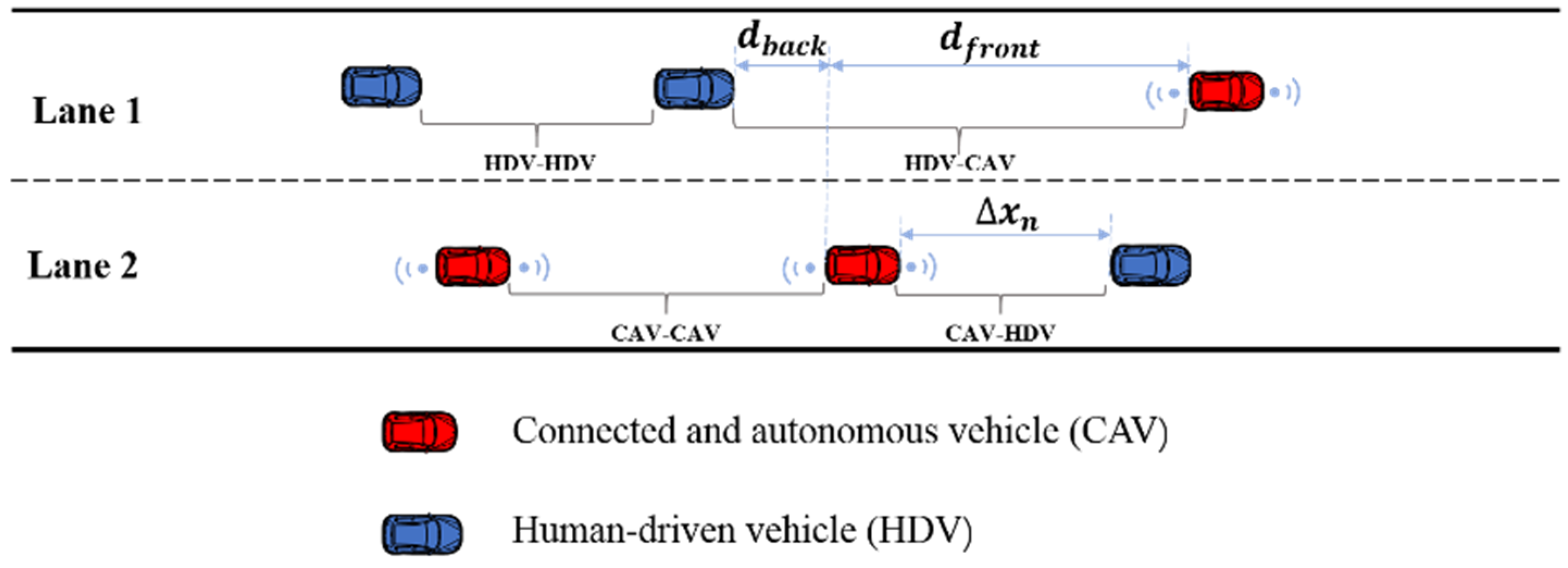
The impact of foggy weather on drivers is mainly reflected in the following three aspects: the reduction in visibility leads to the limited visual distance of the driver, the increase in the driver’s reaction time will increase the safety distance, and drivers are more cautious in making lane-changing decisions, which leads to the decline of the probability of changing lanes [57]. In this paper, we focused on the car-following and lane-changing behaviors of CAVs and HDVs in a mixed traffic flow on a two-lane highway under foggy conditions. The schematic diagram of the scenario is shown in Figure 1.
In the scenario, HDVs, which are the blue vehicles in the schematic diagram, are entirely human-driven. CAVs, which are the red vehicles in the schematic diagram, can always lead the platoon, mixed with HDVs and CAVs, and exchange the position, velocity, and acceleration with the CAVs in the platoon or near lane. The notation for the modeling of the mixed traffic flow in foggy conditions are shown in Table 1.
3.1. The Car-Following Rules
When CAVs and HDVs coexist on the road at the same time, there are four types of car-following: (1) HDV-following-HDV (HDV–HDV), (2) HDV-following-CAV (HDV–CAV), (3) CAV-following-CAV (CAV–CAV), and (4) CAV-following-HDV (CAV-HDV). As HDVs cannot receive real-time information from the leading vehicle, the car-following behavior just depends on the human driver. Therefore, it is believed the car-following strategies are identical for the HDV–HDV and HDV–CAV types. In this paper, we considered three types of car-following in mixed traffic flow: (1) HDV–HDV/CAV, (2) CAV–CAV, (3) CAV–HDV. These three types of car-following strategies in foggy environments are discussed in the following sections in detail.
3.1.1. HDV–HDV/CAV
For an HDV following HDV or CAV, the following strategies were designed as follows.
- Acceleration.
- (1)
- When , and the preceding vehicle is in the scope of visibility, which means , if , then the HDV will accelerate with the probability according to the following acceleration rule:
- (2)
- When , and the preceding vehicle is not in the scope of visibility, which means , then the HDV will adjust its speed within the visible distance. The acceleration rule is as follows:
- Deceleration.
- (1)
- When , if , the HDV will decelerate to ensure safety:
- (2)
- When , if , the HDV cannot judge the distance to the preceding vehicle. In that case, the HDV can adjust its speed within its visible distance to ensure traffic safety; the speed of the vehicle at the next timestep is defined as
- Randomization.HDV slows down randomly according to Equation (5) with the probability .
- Update position.The state of the HDV in this situation from time to can be described as
3.1.2. CAV–CAV
Traffic information inter-transfer and sharing between CAVs can be achieved in CAV following CAV scenarios. We assumed that the CAVs could form a stable fleet with a safety distance. The car-following rules in this situation can be divided into before and after the fleet formation.
Before forming the fleet, if , the CAV will adjust its speed to keep a safe distance from its preceding vehicle as
If , the two CAVs will become a stable fleet with the same speed, which can be described as
After obtaining the fleet, the CAVs update their position with Equation (6).
3.1.3. CAV-HDV
For a CAV following an HDV, there is no communication between the two vehicles. However, the CAV could obtain the status information of its preceding vehicle through its onboard sensing system. When the driving states of surrounding vehicles change, the CAV can quickly sense this and take corresponding measures. In addition, CAVs are barely affected by the reduced visibility. The car-following rules can be modeled as follows:
- Acceleration.If
- Deceleration.If
There is no random slowdown process for a CAV in this situation. Similarly, after obtaining the speed of the subject vehicle, Equation (6) is used to update its position.
3.2. The Lane-Changing Rules
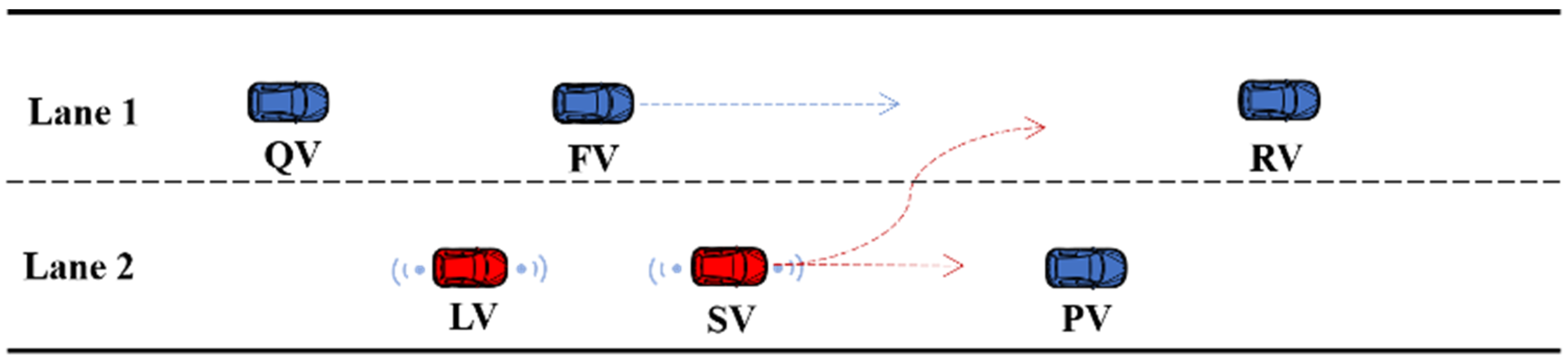
In the process of lane-changing, the driver is greatly affected by the surrounding environment. For instance, drivers will be more cautious and try to reduce lane-changing due to the low visibility. In addition, the state of surrounding vehicles also affects the lane-changing vehicle. Therefore, it is necessary to consider both the safety constraints and the influence of surrounding vehicles in the process of lane-changing. Figure 2 shows a common lane-changing scenario on a two-lane highway.
In Figure 2, the subject vehicle (SV) is driving on Lane 2, and its preceding vehicle (PV) is moving at a slow speed. There is a significant gap in the adjacent lane (Lane 1); the SV may decide to change its driving lanes. The critical difference between HDVs and CAVs is that CAVs could obtain the state of surrounding vehicles and exchange information with neighboring CAVs to accomplish a more flexible lane-changing. Therefore, we designed different lane-changing strategies for HDVs and CAVs in this study.
3.2.1. The Lane-Changing Rules for HDVs
In this CA model, we divide each timestep into two sub-steps: the first sub-step is to apply lane-changing rules to the vehicle and the second sub-step is to update the vehicle’s position on the road. In the symmetric two-lane cellular automaton (STCA) model proposed by Chowdhury, et al. [60], for the decision to change lanes, incentive and safety criteria as shown in Equations (11)–(13) should be satisfied. In the above formulas, Equations (11) and (12) are incentive criteria, meaning the current front spacing is not large enough; Equation (13) is the security criterion which means the target lane has adequate spacing for lane-changing. In this case, the lagging vehicle in the target lane would not have to decelerate too much when the subject vehicle performs lane-changing. When Equations (11)–(13) are satisfied, the HDV will change lanes with a probability of , and the probability is affected by the visibility level. After the vehicle has decided whether to change lanes or not, all vehicles update their speeds and positions according to the car-following rules presented in the above section.
3.2.2. The Lane-Changing Rules for CAVs
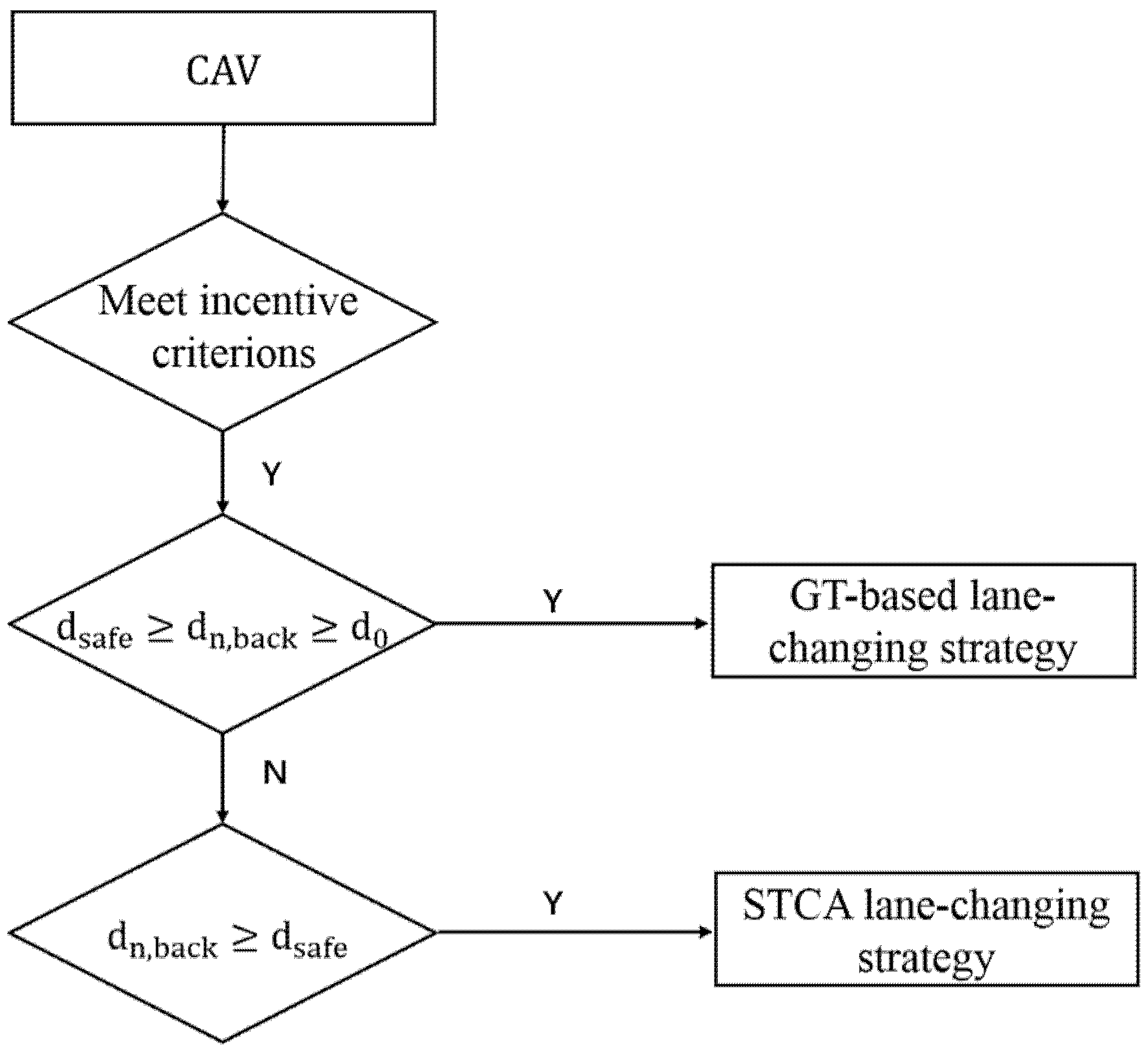
In this section, we proposed a game theory (GT)-based lane-changing policies for CAV. Due to V2V communication, CAVs can obtain detailed information, strategic space, and the payoffs of surrounding vehicles. Therefore, lane-changing behavior is considered to be a non-cooperative game behavior; CAVs can choose the driving strategy according to the payoffs. However, the subject vehicle does not need a lane-changing game in all cases. We believe that only when there is a significant interaction between the subject vehicle and the lagging vehicle in the target lane is a lane-changing game required. Therefore, this paper considers two situations for the lane-changing of CAVs. The first is that the CAV could perform lane changing when Equations (11)–(13) are satisfied, and is assumed to be 1. Since CAVs can complete a safe lane change in a shorter time, they are more willing to change lanes. Thus, the second situation is that a CAV can make lane-changing decisions through game theory in the range of (which is set equal to 2-cell lengths) to [61]. The process of making a CAV is shown in Figure 3.
For a lane-changing vehicle SV, the driving states of its preceding vehicle PV and lagging vehicle LV in the current lane and new preceding vehicle FV and new lagging vehicle RV in the target lane should be primarily considered in the process of lane-changing decision making. Additionally, the vehicle SV will not be affected by its lagging vehicle LV because we believe the vehicle LV will obey the safe car-following rules. Once performing the lane-changing behavior, the new lagging vehicle FV in the target lane may have impacts on vehicle SV’s safety, and the new leading vehicle RV will affect its speed. When the lane-changing game begins, the subject vehicle SV could adopt two strategies: changing lanes or not changing lanes, and we set as the probability that vehicle SV chooses to change lanes. For these two strategies of the vehicle SV, the lagging vehicle FV in the target lane could adopt two pure strategies of acceleration or deceleration, and we set as the probability that vehicle FV selects to accelerate. Note that the lagging vehicle can adopt more pure strategies such as doing nothing (ignoring the lane-changing of vehicle SV), and forced yield (in case the subject vehicle SV executes a forced lane change); however, due to simplicity, this study considers a general deceleration strategy that incorporates all the above-mentioned cases. In our study, the preceding and lagging vehicles of the subject vehicle on the current and target lanes are considered in the calculation of payoffs because they are influenced by the SV’s lane-changing decisions. The structure of the lane-changing game is shown in Table 2.
The calculation formula of payoff was defined as
is defined as the payoff of vehicle SV, where = (1: change lanes, 2: not change lanes); and is defined as the payoff of vehicle FV, where = (1: accelerate, 2: decelerate). In this paper, the payoff function is determined by the acceleration space that may be obtained in the case of vehicle safety. is the relative distance between the target vehicle and its preceding vehicle divided by their relative speed. is the relative distance between the subject vehicle and its following vehicle divided by their relative speed. For example, when vehicle SV chooses to change lanes and vehicle RV selects to accelerate, is the ratio of the distance between vehicle SV and RV to their relative speed after SV completes the lane changing; is the ratio of the distance between vehicle FV and SV to their relative speed after SV changes lanes and FV accelerates. and are, respectively, the weight coefficient and the variation between different driving styles, such as conservative and aggressive. The larger the , the larger the payoff obtained by the driver performing acceleration. In this paper, we default to the neutral driving behavior of vehicles, thus, we set = = 0.5. It is also an interesting topic to consider the CAVs with different preferences, but we will not go into such detail in this article. It is worth noting that if vehicle SV does not choose to change lanes, the impact of the lagging vehicle FV on the SV is negligible, as and were set as = 1, = 0. The expected payoffs of vehicles SV and FV are defined below.
By differentiating Equations (15) and (16) concerning and , respectively, and setting the derivatives equal to zero, the optimal probabilities of action for each player could be obtained:
By maximizing and to obtain the optimal selection of and , which is recorded as and . vehicle SV and vehicle FV must follow the above-mentioned probabilities and for random selection, respectively, to obtain the Nash equilibrium of the mixed strategy game.
4. Numerical and Simulation Experiments
4.1. Scenarios and Setting
The mixed traffic flow of HDVs and CAVs on a two-lane road was simulated using MATLAB. Each lane is 2 km long with 400 cells, and the length of one cell is 5 m. Our CA model adopts the periodic boundary condition to strictly control the vehicle density: once the vehicle leaves the end of the road, it will re-enter the road from the starting point. All the vehicles are generated on the road randomly with different initial speeds, positions, and vehicle types (HDV or CAV). To study the characteristics of mixed traffic flow in the foggy environment, this paper conducted simulation experiments under three scenarios with different visibility levels: “Scenario 1” (dense fog) with visibility less than 50 m, “Scenario 2” (medium fog) with visibility less than 100 m, and “Scenario 3” (no fog) with visibility more than 500 m. The specific parameters are shown in Table 3.
The CAV market penetration rate is set to 0%, 20%, 40%, 60%, 80%, and 100% to investigate the effects of the proportion of CAVs on the mixed traffic flow. Although the reaction time of CAVs is much shorter than that of HDVs, Yang et al. [55] conducted experiments on CAVs with different reaction times ranging from 0.1 s to 1.5 s, and concluded that the reaction time of a CAV has a negligible effect on the two-lane traffic capacity. Thus, for the convenience of calculation in this paper, the simulation under each density lasted 2000 s with each step of 1 s. Each experiment was run ten times to eliminate random errors. The calculation formulas used in the simulation are given as follows:
4.2. Simulation Results
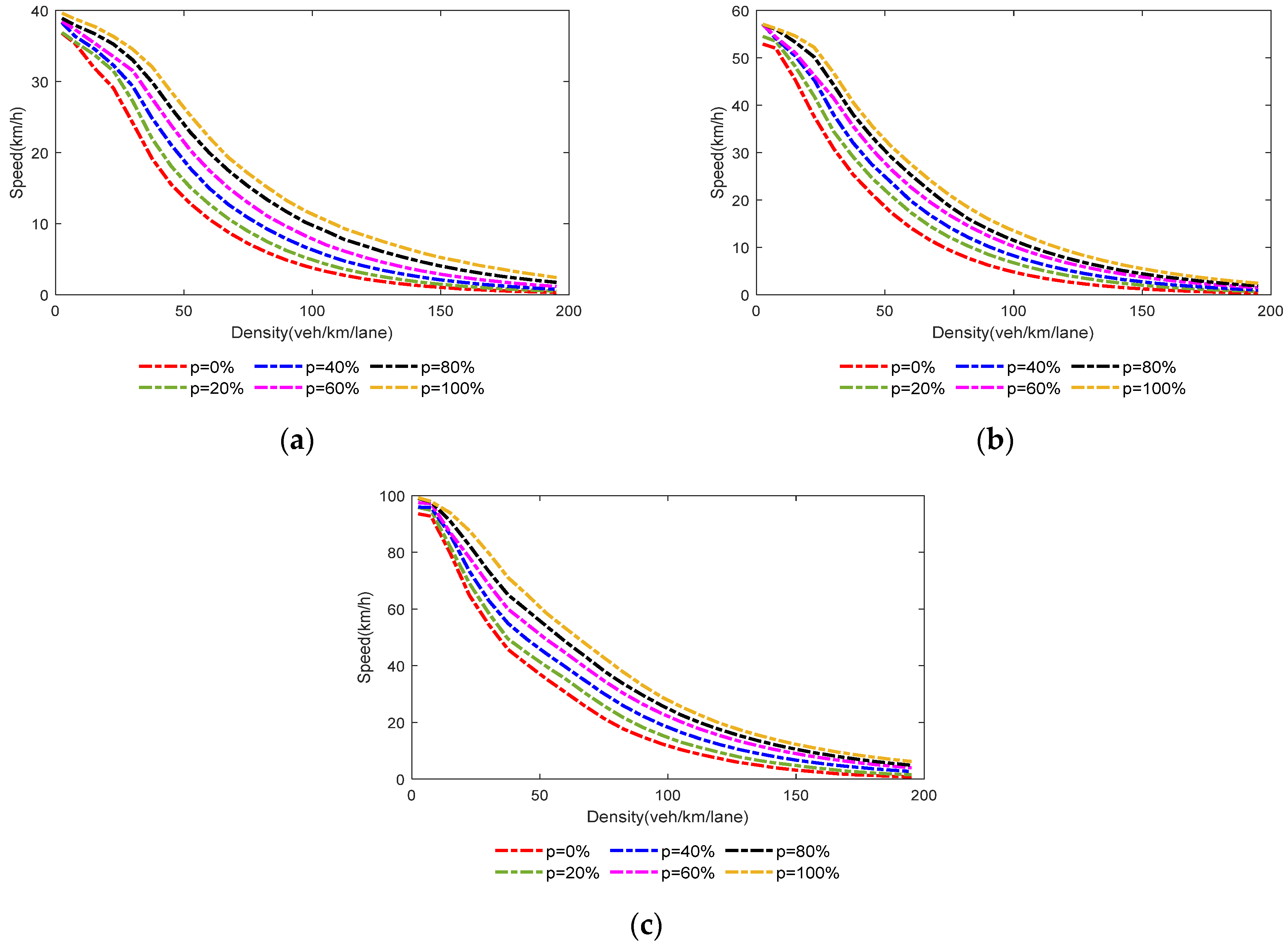
Figure 4 shows the relationship between the average speed for the density under three different visibility levels.
These three scenarios mentioned above were simulated and discussed in this section. Each picture corresponds to a scenario. There are six curves in each figure, showing the simulation results with different CAV penetration rates. This arrangement aims to analyze the possible impact of various CAV penetrations on the traffic flow.
From Figure 4, the decreasing trend of average speed with increasing traffic density. Under free traffic flow on the highway, the average speed is relatively higher in both normal and foggy weather. When there are few vehicles on the highway, there is sufficient space between vehicles to travel at their desired speed without interacting with other vehicles. As vehicle density increases, the further shortening of the average vehicle interval distance would diminish the driver’s expectation of velocity. Therefore, we could find the average speed would show a downward trend. Especially in relatively low density, this trend becomes more obvious. As the density increases, the traffic is characterized by high density and low speed.
Observing the phenomenon of traffic flow in dense fog, we could find that the speed fluctuation in dense fog is relatively tiny. That is because the maximum speed in dense fog is greatly restricted. It can be concluded that the weather factor is more important than the density factor in this situation.
Moreover, the average speed of different CAV proportions was compared under normal weather and foggy weather. It can be seen that the higher the percentage of CAVs implemented, the higher the average speed that could be achieved. In addition, the positive influence of CAVs on the improvement of highway traffic speed is more evident, especially under lower visibility conditions. For example, when the vehicle density = 112.5 veh/km/lane, the average speed increases by 157.8% as the CAV penetration rate grows from 0% to 100% in no fog conditions, while in conditions of dense fog, this value increases by 239%.
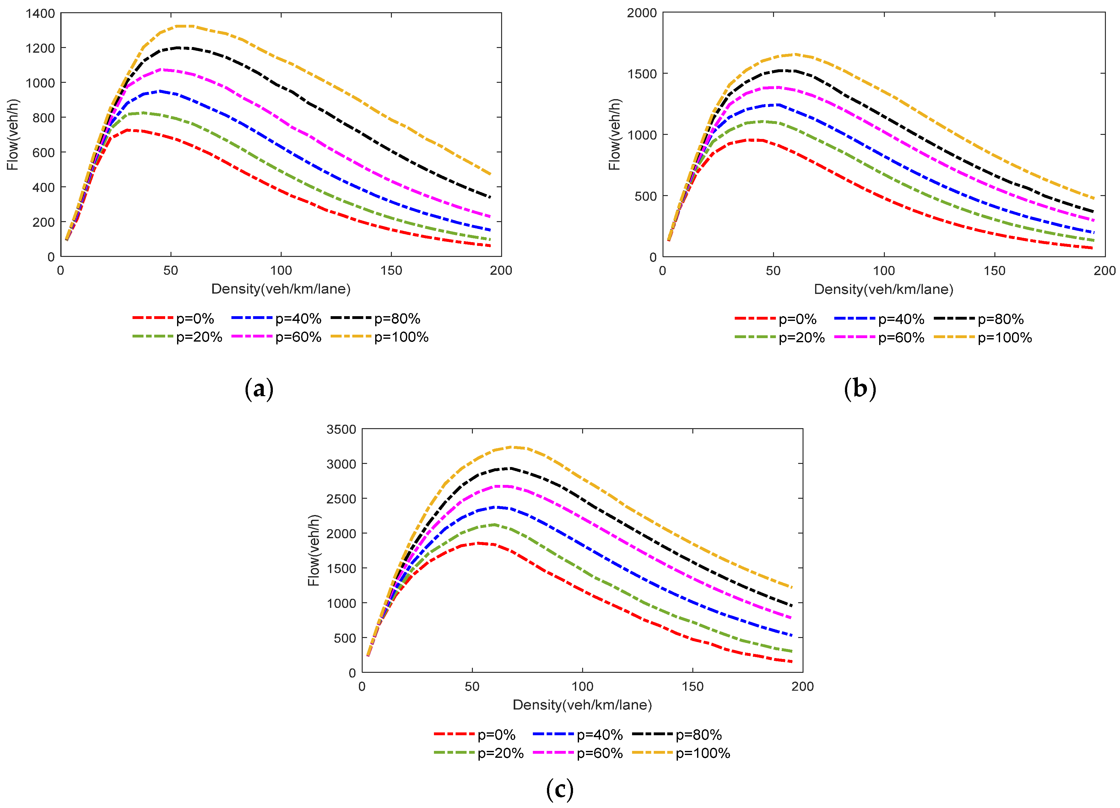
Figure 5 presents the flow–density relation under different visibility levels.
It can be found from Figure 5a–c that the maximum capacity in fog is lower in normal weather; the road capacity decreased 1.55 times as the visible distance reduced from 500 m to 50 m when there are only HDVs on the road. After introducing CAVs, the road capacity increased as the CAV penetration rate increased. This phenomenon is because a CAV has better performance than an HDV, achieving a smaller gap in relation to their preceding vehicle.
Furthermore, the figure indicates that the employment of CAVs is more effective in reduced visibility conditions. For example, when density = 112.5 veh/km/lane, as CAV penetration rate increases from 0% to 100%, the traffic capacity increases by 239.4% in dense fog scenarios while increasing by 157.9% in clear weather.
For different CAV penetration rates, the density range of the free flow phase is also diverse. As the proportion of CAVs increases, the corresponding density with maximum road capacity will increase, indicating that the introduction of CAVs could increase the critical density.
Figure 6 shows the variation in traffic capacity as the density increases under different visibility levels.
Each subplot represents a case with a fixed CAV penetration rate, and the range of is from 0% to 100%. As shown in Figure 6a, when the vehicle density reaches 45 veh/km/lane, the traffic capacity in no fog condition is 2.61 times than that in a condition of dense fog. In addition, with the proportion of CAV keeps unchanged, the free-flow density ranges under different visibility levels are different. The critical density in conditions of dense fog is smaller than that in conditions of no fog. For example, in Figure 6a, we can find that the relationship between critical density in dense fog , in medium fog and in no fog is . Particularly in cases with a relatively lower CAV penetration rate, the free-flow density range under dense foggy environment is much smaller than that in no fog condition. As the CAV proportion increases, this gap gradually narrows, indicating that the introduction of CAVs has a greater improvement in critical density under foggy conditions.
4.3. Comparison with Other Work
To evaluate the performance of the proposed models, the simulation results were compared with the traditional STCA lane-changing strategy published by Chowdhury, Wolf, and Schreckenberg [60]. In the comparison, we change merely the lane-changing strategies for vehicles and keep other settings unchanged. We conducted experiments under three traffic flow conditions: low-density ( = 15 veh/km/lane), medium-density ( = 75 veh/km/lane), and high-density traffic flow ( = 135 veh/km/lane). Table 4 illustrates the summary of the comparison of the average speed with these two lane-changing strategies under different traffic flow density stages in dense fog and no fog conditions.
As we can see in the table, compared with traditional STCA lane-changing rules, the lane-changing strategy proposed in this paper could increase the overall speed of traffic. In the low-density phase, the speed difference in these two strategies is slight under various visibility levels. This phenomenon is because the vehicle could drive at the expected speed in the free-flow phase, and there is little need to change lanes for a higher speed.
In medium-density, the difference in speed between these two strategies becomes larger in dense fog and no fog conditions. In this case, as the vehicle density increases, many vehicles hope for a more efficient driving environment. Therefore, lane-changing for a higher speed was chosen. The results showed that the average speed in the proposed lane-changing strategy is much higher, indicating that the GT-based lane-changing strategy has advantages.
When the vehicle density is high, the speed difference between these two strategies becomes negligible. In this situation, traffic density is the main factor affecting the velocity. The road is getting congested, and a vehicle can hardly change lanes in this situation, so the advantages of the proposed model become less pronounced.
In summary, the lane-changing rules in STCA model are relatively fixed and the rules overemphasize safety, which makes CAVs’ lane-changing efficiency low. The GT-based lane-changing strategies for CAVs proposed in this paper can not only ensure safety during lane-changing, but also improve the overall speed of the vehicles and further reduce delays.
5. Conclusions
A comprehensive understanding of mixed traffic characteristics in foggy environments could help to limit the occurrence and impact of traffic accidents. Therefore, a novel CA model is presented in this paper to model the mixed traffic flow of CAVs and HDVs in fog. Firstly, we proposed different car-following strategies for different vehicle combinations in foggy conditions. Following this, we designed different lane-changing rules for CAVs and HDVs. We used a rule-based lane-changing approach for HDVs and applied the game theory to the lane-changing strategy for CAVs. Finally, we used the proposed CA model to simulate the traffic flow under different visibility levels. In addition, based on different market penetration rates of CAVs, we presented a three-phase diagram of mixed traffic flow, which can be applied to various scenarios of mixed traffic flow under different visible distances.
The analytical studies revealed that the impact of reduced visibility on the traffic reflects the reduction in average speed and traffic capacity. In addition, the free-flow density range under the condition of dense fog is much smaller than that in a no fog condition. The introduction of CAVs is beneficial to traffic efficiency (e.g., average vehicle speed and traffic capacity). In addition, with increases in the penetration of CAVs deployed on the road, the critical density increases, and this phenomenon is more evident in foggy conditions.
However, it should be pointed out that the proposed model has some limitations. The first limitation is that there are no available field data to verify the model due to the lack of large-scale experimental data for connected vehicles in fog. The second limitation is that some factors such as communication delay and road friction coefficient should be considered in the model. The third limitation is that in the proposed lane-changing model, only the communication between the subject CAV and its adjacent vehicles is considered, in fact communication with further vehicles could be considered, which will strengthen fleet formation and increase road capacity.
Author Contributions
Conceptualization, B.G.; methodology, F.W.; software, F.W.; validation, D.W.; resources, C.L.; writing—original draft preparation, F.W.; writing—review and editing, B.G., C.L., and D.W.; supervision, B.G. All authors have read and agreed to the published version of the manuscript.
Funding
This research was funded by the Scientific Research Project of the Education Department of Jilin Province (Grant No. JJKH20221020KJ), the Jilin Province Transportation Innovation and Development Support (Science and Technology) Project (Grant No. 2021-1-11), and the Key Laboratory of Transport Industry of Big Data Application Technologies for Comprehensive Transport, Ministry of Transport, China Academy of Transportation Science (Grant No. 2021B1206) are partly supporting this work.
Institutional Review Board Statement
Not applicable.
Informed Consent Statement
Not applicable.
Data Availability Statement
Data are available from the corresponding author upon request.
Conflicts of Interest
The authors declare no conflict of interest.
References
- Talebpour, A.; Mahmassani, H. Influence of connected and autonomous vehicles on traffic flow stability and throughput. Transp. Res.-Emerg. Technol. 2016, 71, 143–163. [Google Scholar] [CrossRef]
- Chen, D.; Ahn, S.; Chitturi, M.; Noyce, D. Towards vehicle automation: Roadway capacity formulation for traffic mixed with regular and automated vehicles. Transp. Res.-Methodol. 2017, 100, 196–221. [Google Scholar] [CrossRef] [Green Version]
- Bahrami, S.; Roorda, M. Optimal traffic management policies for mixed human and automated traffic flows. Transp. Res.-Policy Pract. 2020, 135, 130–143. [Google Scholar] [CrossRef]
- Cao, Z.; Lu, L.; Chen, C.; Chen, X. Modeling and Simulating Urban Traffic Flow Mixed With Regular and Connected Vehicles. IEEE Access 2021, 9, 10392–10399. [Google Scholar] [CrossRef]
- Wang, Y.; Liang, L.; Evans, L. Fatal crashes involving large numbers of vehicles and weather. J. Saf. Res. 2017, 63, 1–7. [Google Scholar] [CrossRef]
- Zhang, X.; Gao, J. Research on the fixation transition behavior of drivers on expressway in foggy environment. Saf. Sci. 2019, 119, 70–75. [Google Scholar]
- Zhao, C.; Jiang, S.; Lei, Y.; Wang, C. A Study on an Anthropomorphic Car-Following Strategy Framework of the Autonomous Coach in Mixed Traffic Flow. IEEE Access 2020, 8, 64653–64665. [Google Scholar] [CrossRef]
- Chen, C.; Wang, J.; Xu, Q.; Wang, J.; Li, K. Mixed platoon control of automated and human-driven vehicles at a signalized intersection: Dynamical analysis and optimal control. Transp. Res.-Emerg. Technol. 2021, 127, 103138. [Google Scholar] [CrossRef]
- Hidalgo, C.; Lattarulo, R.; Flores, C.; Perez Rastelli, J. Platoon Merging Approach Based on Hybrid Trajectory Planning and CACC Strategies. Sensors 2021, 21, 2626. [Google Scholar] [CrossRef]
- Liu, H.; Kan, X.; Shladover, S.; Lu, X.; Ferlis, R. Modeling impacts of Cooperative Adaptive Cruise Control on mixed traffic flow in multi-lane freeway facilities. Transp. Res.-Emerg. Technol. 2018, 95, 261–279. [Google Scholar] [CrossRef]
- Zheng, F.; Liu, C.; Liu, X.; Jabari, S.; Lu, L. Analyzing the impact of automated vehicles on uncertainty and stability of the mixed traffic flow. Transp. Res.-Emerg. Technol. 2020, 112, 203–219. [Google Scholar] [CrossRef]
- Li, C.; Feng, H.; Zhi, X.; Zhao, N. Intelligent guidance system for foggy area traffic safety operation. In Proceedings of the 2011 14th International IEEE Conference on Intelligent Transportation Systems (ITSC), Washington, DC, USA, 5–7 October 2011; pp. 428–432. [Google Scholar]
- Yan, X.; Li, X.; Liu, Y.; Zhao, J. Effects of foggy conditions on drivers’ speed control behaviors at different risk levels. Saf. Sci. 2014, 68, 275–287. [Google Scholar] [CrossRef]
- Saffarian, M.; Happee, R.; Winter, J. Why do drivers maintain short headways in fog? A driving-simulator study evaluating feeling of risk and lateral control during automated and manual car following. Ergonomics 2012, 55, 971–985. [Google Scholar] [CrossRef] [PubMed]
- Hoogendoorn, R.; Tamminga, G.; Hoogendoorn, S.; Daamen, W. Longitudinal driving behavior under adverse weather conditions: Adaptation effects, model performance and freeway capacity in case of fog. In Proceedings of the 13th International IEEE Conference on Intelligent Transportation Systems, Funchal, Portugal, 19–22 September 2010; pp. 450–455. [Google Scholar]
- Broughton, K.; Switzer, F.; Scott, D. Car following decisions under three visibility conditions and two speeds tested with a driving simulator. Accid. Anal. Prev. 2007, 39, 106–116. [Google Scholar] [CrossRef]
- Peng, Y.; Abdel-Aty, M.; Shi, Q.; Yu, R. Assessing the impact of reduced visibility on traffic crash risk using microscopic data and surrogate safety measures. Transp. Res.-Emerg. Technol. 2017, 74, 295–305. [Google Scholar] [CrossRef] [Green Version]
- Deng, C.; Wu, C.; Cao, S.; Lyu, N. Modeling the effect of limited sight distance through fog on car-following performance using QN-ACTR cognitive architecture. Transp. Res.-Traffic Psychol. Behav. 2019, 65, 643–654. [Google Scholar] [CrossRef]
- Gao, K.; Tu, H.; Sun, L.; Sze, N.; Song, Z.; Shi, H. Impacts of reduced visibility under hazy weather condition on collision risk and car-following behavior: Implications for traffic control and management. Int. J. Sustain. Transp. 2019, 14, 635–642. [Google Scholar] [CrossRef]
- Gong, B.; Wei, R.; Wu, D.; Lin, C. Fleet Management for HDVs and CAVs on Highway in Dense Fog Environment. J. Adv. Transp. 2020, 2020, 8842730. [Google Scholar] [CrossRef]
- Ye, L.; Yamamoto, T. Modeling connected and autonomous vehicles in heterogeneous traffic flow. Phys. Stat. Mech. Appl. 2018, 490, 269–277. [Google Scholar] [CrossRef]
- Jafaripournimchahi, A.; Hu, W.; Sun, L. An Asymmetric-Anticipation Car-following Model in the Era of Autonomous-Connected and Human-Driving Vehicles. J. Adv. Transp. 2020, 2020, 8865814. [Google Scholar] [CrossRef]
- Wang, M.; Daamen, W.; Hoogendoorn, S.; van Arem, B. Rolling horizon control framework for driver assistance systems. Part II: Cooperative sensing and cooperative control. Transp. Res.-Emerg. Technol. 2014, 40, 290–311. [Google Scholar] [CrossRef]
- Milanes, V.; Shladover, S.; Spring, J.; Nowakowski, C.; Kawazoe, H.; Nakamura, M. Cooperative Adaptive Cruise Control in Real Traffic Situations. IEEE Trans. Intell. Transp. Syst. 2014, 15, 296–305. [Google Scholar] [CrossRef] [Green Version]
- Treiber, M.; Hennecke, A.; Helbing, D. Congested traffic states in empirical observations and microscopic simulations. Phys. Rev. Stat. Phys. Plasmas Fluids Relat. Interdiscip. Top. 2000, 62, 1805–1824. [Google Scholar] [CrossRef] [PubMed] [Green Version]
- Shladover, S.; Su, D.; Lu, X. Impacts of Cooperative Adaptive Cruise Control on Freeway Traffic Flow. Transp. Res. Rec. 2012, 2324, 63–70. [Google Scholar] [CrossRef] [Green Version]
- Milanés, V.; Shladover, S. Modeling cooperative and autonomous adaptive cruise control dynamic responses using experimental data. Transp. Res. Emerg. Technol. 2014, 48, 285–300. [Google Scholar] [CrossRef] [Green Version]
- Chen, N.; Wang, M.; Alkim, T.; van Arem, B. A Robust Longitudinal Control Strategy of Platoons under Model Uncertainties and Time Delays. J. Adv. Transp. 2018, 2018, 9852721. [Google Scholar] [CrossRef] [Green Version]
- Li, F.; Wang, Y. Cooperative Adaptive Cruise Control for String Stable Mixed Traffic: Benchmark and Human-Centered Design. IEEE Trans. Intell. Transp. Syst. 2017, 18, 3473–3485. [Google Scholar] [CrossRef]
- Gong, S.; Du, L. Cooperative platoon control for a mixed traffic flow including human drive vehicles and connected and autonomous vehicles. Transp. Res.-Methodol. 2018, 116, 25–61. [Google Scholar] [CrossRef]
- Karoui, O.; Khalgui, M.; Koubaa, A.; Guerfala, E.; Li, Z.; Tovar, E. Dual mode for vehicular platoon safety: Simulation and formal verification. Inf. Sci. 2017, 402, 216–232. [Google Scholar] [CrossRef]
- Nie, L.; Guan, J.; Lu, C.; Zheng, H.; Yin, Z. Longitudinal speed control of autonomous vehicle based on a self-adaptive PID of radial basis function neural network. IET Intell. Transp. Syst. 2018, 12, 485–494. [Google Scholar] [CrossRef]
- Gupta, A.; Anpalagan, A.; Guan, L.; Khwaja, A.S. Deep learning for object detection and scene perception in self-driving cars: Survey, challenges, and open issues. Array 2021, 10, 100057. [Google Scholar] [CrossRef]
- Olovsson, T.; Svensson, T.; Wu, J. Future connected vehicles: Communications demands, privacy and cyber-security. Commun. Transp. Res. 2022, 2, 100056. [Google Scholar] [CrossRef]
- Peng, B.; Keskin, M.F.; Kulcsár, B.; Wymeersch, H. Connected autonomous vehicles for improving mixed traffic efficiency in unsignalized intersections with deep reinforcement learning. Commun. Transp. Res. 2021, 1, 100017. [Google Scholar] [CrossRef]
- Wang, P.; Chan, C.Y.; Fortelle, A. A Reinforcement Learning Based Approach for Automated Lane Change Maneuvers. In Proceedings of the 2018 IEEE Intelligent Vehicles Symposium, Changshu, China, 26–30 June 2018. [Google Scholar]
- Kang, K.; Rakha, H. Game Theoretical Approach to Model Decision Making for Merging Maneuvers at Freeway On-Ramps. Transp. Res. Rec. 2017, 2623, 19–28. [Google Scholar] [CrossRef]
- Hang, P.; Lv, C.; Xing, Y.; Huang, C.; Hu, Z. Human-Like Decision Making for Autonomous Driving: A Noncooperative Game Theoretic Approach. IEEE Trans. Intell. Transp. Syst. 2021, 22, 2076–2087. [Google Scholar] [CrossRef]
- Wang, M.; Hoogendoorn, S.; Daamen, W.; van Arem, B.; Happee, R. Game theoretic approach for predictive lane-changing and car-following control. Transp. Res.-Emerg. Technol. 2015, 58, 73–92. [Google Scholar] [CrossRef]
- Yu, H.; Tseng, H.; Langari, R. A human-like game theory-based controller for automatic lane changing. Transp. Res.-Emerg. Technol. 2018, 88, 140–158. [Google Scholar] [CrossRef]
- Talebpour, A.; Mahmassani, H.; Hamdar, S. Modeling lane-changing behavior in a connected environment: A game theory approach. Transp. Res. Emerg. Technol. 2015, 59, 216–232. [Google Scholar] [CrossRef]
- Lin, D.; Li, L.; Jabari, S. Pay to change lanes: A cooperative lane-changing strategy for connected/automated driving. Transp. Res.-Emerg. Technol. 2019, 105, 550–564. [Google Scholar] [CrossRef] [Green Version]
- Tian, J.; Zhu, C.; Jiang, R.; Treiber, M. Review of the cellular automata models for reproducing synchronized traffic flow. Transp. Transp. Sci. 2020, 17, 766–800. [Google Scholar] [CrossRef]
- Muhammad, T.; Kashmiri, F.; Naeem, H.; Qi, X.; Chia-Chun, H.; Lu, H. Simulation Study of Autonomous Vehicles’ Effect on Traffic Flow Characteristics including Autonomous Buses. J. Adv. Transp. 2020, 2020, 4318652. [Google Scholar] [CrossRef]
- Nagel, K.; Schreckenberg, M. A cellular automaton model for freeway traffic. J. Phys. 1992, 2, 2221–2229. [Google Scholar] [CrossRef]
- Takayasu, M.; Takayasu, H. 1/f noise in a traffic model. Fractals 1993, 1, 860–866. [Google Scholar] [CrossRef]
- Ning, W.U.; Brilon, W. Cellular Automata for Highway Traffic Flow Simulation. 1999. Available online: https://www.researchgate.net/publication/255571908_Cellular_Automata_for_Highway_Traffic_Flow_Simulation (accessed on 1 January 1999).
- Li, X.; Wu, Q.; Jiang, R. Cellular automaton model considering the velocity effect of a car on the successive car. Phys. Rev. 2001, 64, 066128. [Google Scholar] [CrossRef]
- Habel, L.; Schreckenberg, M. Asymmetric lane change rules for a microscopic highway traffic model. In Proceedings of the International Conference on Cellular Automata, Krakow, Poland, 22–25 September 2014; Springer: Berlin/Heidelberg, Germany, 2014; pp. 620–629. [Google Scholar]
- Pottmeier, A.; Thiemann, C.; Schadschneider, A.; Schreckenberg, M. Mechanical restriction versus human overreaction: Accident avoidance and two-lane traffic simulations. In Traffic and Granular Flow’05; Springer: Berlin/Heidelberg, Germany, 2007; pp. 503–508. [Google Scholar]
- Chen, B.; Sun, D.; Zhou, J.; Wong, W.; Ding, Z. A future intelligent traffic system with mixed autonomous vehicles and human-driven vehicles. Inf. Sci. 2020, 529, 59–72. [Google Scholar] [CrossRef]
- Hu, X.; Huang, M.; Guo, J. Feature Analysis on Mixed Traffic Flow of Manually Driven and Autonomous Vehicles Based on Cellular Automata. Math. Probl. Eng. 2020, 2020, 7210547. [Google Scholar] [CrossRef]
- Vranken, T.; Sliwa, B.; Wietfeld, C.; Schreckenberg, M. Adapting a cellular automata model to describe heterogeneous traffic with human-driven, automated, and communicating automated vehicles. Phys.-Stat. Mech. Appl. 2021, 570, 125792. [Google Scholar] [CrossRef]
- Gipps, P. A behavioural car-following model for computer simulation. Transp. Res. Methodol. 1981, 15, 105–111. [Google Scholar] [CrossRef]
- Yang, D.; Qiu, X.; Ma, L.; Wu, D.; Zhu, L.; Liang, H. Cellular Automata-Based Modeling and Simulation of a Mixed Traffic Flow of Manual and Automated Vehicles. Transp. Res. Rec. 2017, 2622, 105–116. [Google Scholar] [CrossRef]
- Vranken, T.; Schreckenberg, M. Modelling multi-lane heterogeneous traffic flow with human-driven, automated, and communicating automated vehicles. Phys.-Stat. Mech. Appl. 2022, 589, 126629. [Google Scholar] [CrossRef]
- Das, A.; Ahmed, M.M. Exploring the effect of fog on lane-changing characteristics utilizing the SHRP2 naturalistic driving study data. J. Transp. Saf. Secur. 2021, 13, 477–502. [Google Scholar] [CrossRef]
- Levin, M.W.; Boyles, S.D. A multiclass cell transmission model for shared human and autonomous vehicle roads. Transp. Res. Emerg. Technol. 2016, 62, 103–116. [Google Scholar] [CrossRef] [Green Version]
- Tanveer, M.; Kashmiri, F.A.; Yan, H.; Wang, T.; Lu, H. A Cellular Automata Model for Heterogeneous Traffic Flow Incorporating Micro Autonomous Vehicles. J. Adv. Transp. 2022, 2022, 8815026. [Google Scholar] [CrossRef]
- Chowdhury, D.; Wolf, D.; Schreckenberg, M. Particle hopping models for two-lane traffic with two kinds of vehicles: Effects of lane-changing rules. Phys.-Stat. Mech. Appl. 1997, 235, 417–439. [Google Scholar] [CrossRef]
- Fei, L.; Zhu, H.; Han, X. Analysis of traffic congestion induced by the work zone. Phys.-Stat. Mech. Appl. 2016, 450, 497–505. [Google Scholar] [CrossRef]
Figure 1.
The schematic of the simulation system.

Figure 2.
The lane-changing scenario.

Figure 3.
The process of lane-changing for CAV.

Figure 4.
Speed-density diagrams under different CAV market penetration . (a) dense fog condition ( = 50 m), (b) medium fog condition ( = 100 m), (c) no fog condition ( = 500 m).
Figure 4.
Speed-density diagrams under different CAV market penetration . (a) dense fog condition ( = 50 m), (b) medium fog condition ( = 100 m), (c) no fog condition ( = 500 m).

Figure 5.
Flow-density diagrams under different CAV market penetration . (a) Dense fog condition ( = 50 m), (b) medium fog condition ( = 100 m), (c) no fog condition ( = 500 m).
Figure 5.
Flow-density diagrams under different CAV market penetration . (a) Dense fog condition ( = 50 m), (b) medium fog condition ( = 100 m), (c) no fog condition ( = 500 m).

Figure 6.
Flow–density diagrams under different visibility levels. (a) , (b) , (c) , (d) , (e) , (f) .
Figure 6.
Flow–density diagrams under different visibility levels. (a) , (b) , (c) , (d) , (e) , (f) .


Table 1.
The notation of model parameters and variables.
| Notion | Explanation |
|---|---|
| the space of the gap between the subject vehicle and the preceding vehicle in the target lane | |
| the space of the gap between the subject vehicle and the succeeding vehicle in the target lane | |
| the space of the gap that needs to be satisfied to be safe | |
| the visible distance in foggy environment | |
| the length of the single lane | |
| the total number of vehicles | |
| the CAV proportion in traffic flow | |
| the lane-changing probability | |
| the acceleration probability | |
| the randomization deceleration probability | |
| the traffic flow | |
| the timestep in the simulation | |
| the simulation time horizon | |
| the maximum speed | |
| the minimum speed | |
| the average speed | |
| the space gap between the subject vehicle and the preceding vehicle in the current lane | |
| the vehicle density |
Table 2.
Payoff matrix for the lane-changing game.
| Decision Making | FV. | ||
|---|---|---|---|
| Accelerate (n) | Decelerate (1 − n) | ||
| SV. | ) | ) | |
| ) | ) | ||
Table 3.
The parameters in the CA model.
| Parameter | Scenario 1 | Scenario 2 | Scenario 3 |
|---|---|---|---|
| 50 | 100 | 500 | |
| 40 | 60 | 100 | |
| 0.2 | 0.3 | 0.4 | |
| 0.4 | 0.2 | 0.1 |
Table 4.
Comparison of model average speed.
| in STCA- | in GT-Based | Increase | in STCA- | in GT-Based | Increase | ||
|---|---|---|---|---|---|---|---|
| (veh/km/h) | LC (km/h) | LC (km/h) | (%) | LC (km/h) | LC (km/h) | (%) | |
| 0% | 29.61 | 31.94 | 7.87 | 71.26 | 73.67 | 3.38 | |
| 20% | 30.97 | 33.49 | 8.13 | 72.09 | 75.85 | 5.22 | |
| 40% | 31.01 | 34.62 | 8.15 | 79.77 | 80.17 | 5.01 | |
| 60% | 32.49 | 35.44 | 8.4 | 81.89 | 85.91 | 4.91 | |
| 80% | 34.03 | 36.76 | 8.02 | 85.09 | 89.99 | 5.76 | |
| 100% | 35.18 | 37.77 | 7.36 | 87.66 | 92.91 | 5.99 | |
| 0% | 4.36 | 7.2 | 65.14 | 11.44 | 21.42 | 87.23 | |
| 20% | 5.29 | 8.91 | 68.43 | 13.39 | 25.86 | 93.13 | |
| 40% | 6.13 | 10.81 | 76.35 | 16.15 | 30.15 | 86.69 | |
| 60% | 7.28 | 12.93 | 77.61 | 17.74 | 34.73 | 95.77 | |
| 80% | 8.49 | 15.26 | 79.74 | 20.73 | 38.2 | 84.27 | |
| 100% | 9.36 | 17.07 | 82.37 | 24.53 | 42.86 | 74.72 | |
| 0% | 1.42 | 1.52 | 7.04 | 3.16 | 4.97 | 57.28 | |
| 20% | 1.85 | 2.12 | 14.59 | 4.47 | 6.68 | 49.44 | |
| 40% | 2.47 | 2.92 | 18.21 | 4.92 | 9.08 | 84.55 | |
| 60% | 3.35 | 3.92 | 17.01 | 6.29 | 11.79 | 87.44 | |
| 80% | 4.56 | 5.32 | 16.67 | 7.42 | 13.62 | 83.56 | |
| 100% | 5.49 | 6.57 | 19.67 | 8.03 | 15.59 | 94.15 | |
Publisher’s Note: MDPI stays neutral with regard to jurisdictional claims in published maps and institutional affiliations. |
© 2022 by the authors. Licensee MDPI, Basel, Switzerland. This article is an open access article distributed under the terms and conditions of the Creative Commons Attribution (CC BY) license (https://creativecommons.org/licenses/by/4.0/).
Share and Cite
MDPI and ACS Style
Gong, B.; Wang, F.; Lin, C.; Wu, D. Modeling HDV and CAV Mixed Traffic Flow on a Foggy Two-Lane Highway with Cellular Automata and Game Theory Model. Sustainability 2022, 14, 5899. https://0-doi-org.brum.beds.ac.uk/10.3390/su14105899
AMA Style
Gong B, Wang F, Lin C, Wu D. Modeling HDV and CAV Mixed Traffic Flow on a Foggy Two-Lane Highway with Cellular Automata and Game Theory Model. Sustainability. 2022; 14(10):5899. https://0-doi-org.brum.beds.ac.uk/10.3390/su14105899
Chicago/Turabian StyleGong, Bowen, Fanting Wang, Ciyun Lin, and Dayong Wu. 2022. "Modeling HDV and CAV Mixed Traffic Flow on a Foggy Two-Lane Highway with Cellular Automata and Game Theory Model" Sustainability 14, no. 10: 5899. https://0-doi-org.brum.beds.ac.uk/10.3390/su14105899
Note that from the first issue of 2016, this journal uses article numbers instead of page numbers. See further details here.