
Driver Behavioral Classification on Curves Based on the Relationship between Speed, Trajectories, and Eye Movements: A Driving Simulator Study


Abstract
:1. Introduction
2. Materials and Methods
2.1. Participants
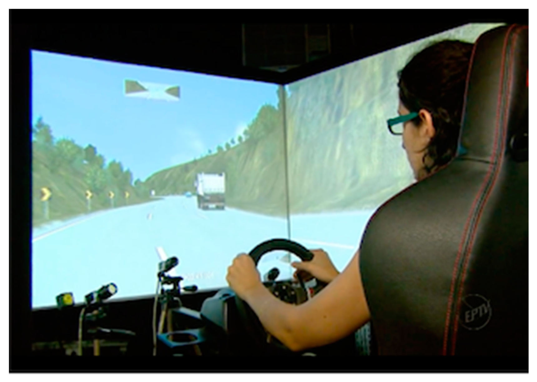
2.2. Apparatus
2.3. Experimental Road
2.4. Database
2.5. Data Analysis
- Description of variables:
- ○
- Dependent variables: driving speed, lateral placement, and eye movement information, such as the number of fixations, fixation duration, pupil diameter, and gaze direction.
- ○
- Independent variables: approach tangent lengths and curve radii.
- Factorial ANOVA is an analysis of variance involving two or more independent variables, which is the case of this experiment, as shown in the descriptions of variables above.
- ANOVA with repeated measures consists of an analysis of variance conducted in any design. The independent (predictor) variables were measured using the same subjects under all conditions, which is the case of our experiment. The F-statistic from a repeated measures ANOVA is reported as F (df, dferror) = F-value, p = p-value. The first degree of freedom (df) was calculated as the number of conditions less one, and the second was the product of the first with the number of subjects less one. The following formula explains the F-ratio:where MS is the mean squared error or the mean variability in the data.
- The following tests were performed to check if the assumptions to proceed with the ANOVA with repeated measures were not violated:
- ○
- The Kolmogorov–Smirnov test evaluates if the distribution of scores is significantly different from a normal distribution. A significant p-value indicates a deviation from normality.
- ○
- The Friedman’s ANOVA is a non-parametric test, also known as the non-parametric version of the one-way repeated measures ANOVA. It compares multiple conditions when the same subjects participate in each condition. The resulting data are not normally distributed.
- ○
- The Levene’s test checks if there is any significant difference between the variances of a group and, thus, a non-significant result indicates that the hypothesis was satisfied.
- ○
- The Mauchly test assesses the hypothesis that the variances of differences between conditions are equal. A significant Mauchly’s statistical test (i.e., when it has a probability value less than 0.05), it is conclusive that there are significant differences between the variances of the differences; therefore, the sphericity condition was violated.
- ■
- The Greenhouse–Geisser correction estimates the distance from sphericity. It was used to correct the degrees of freedom associated with the corresponding F ratio when the Mauchly test causes the sphericity condition to be violated.
3. Results and Discussion
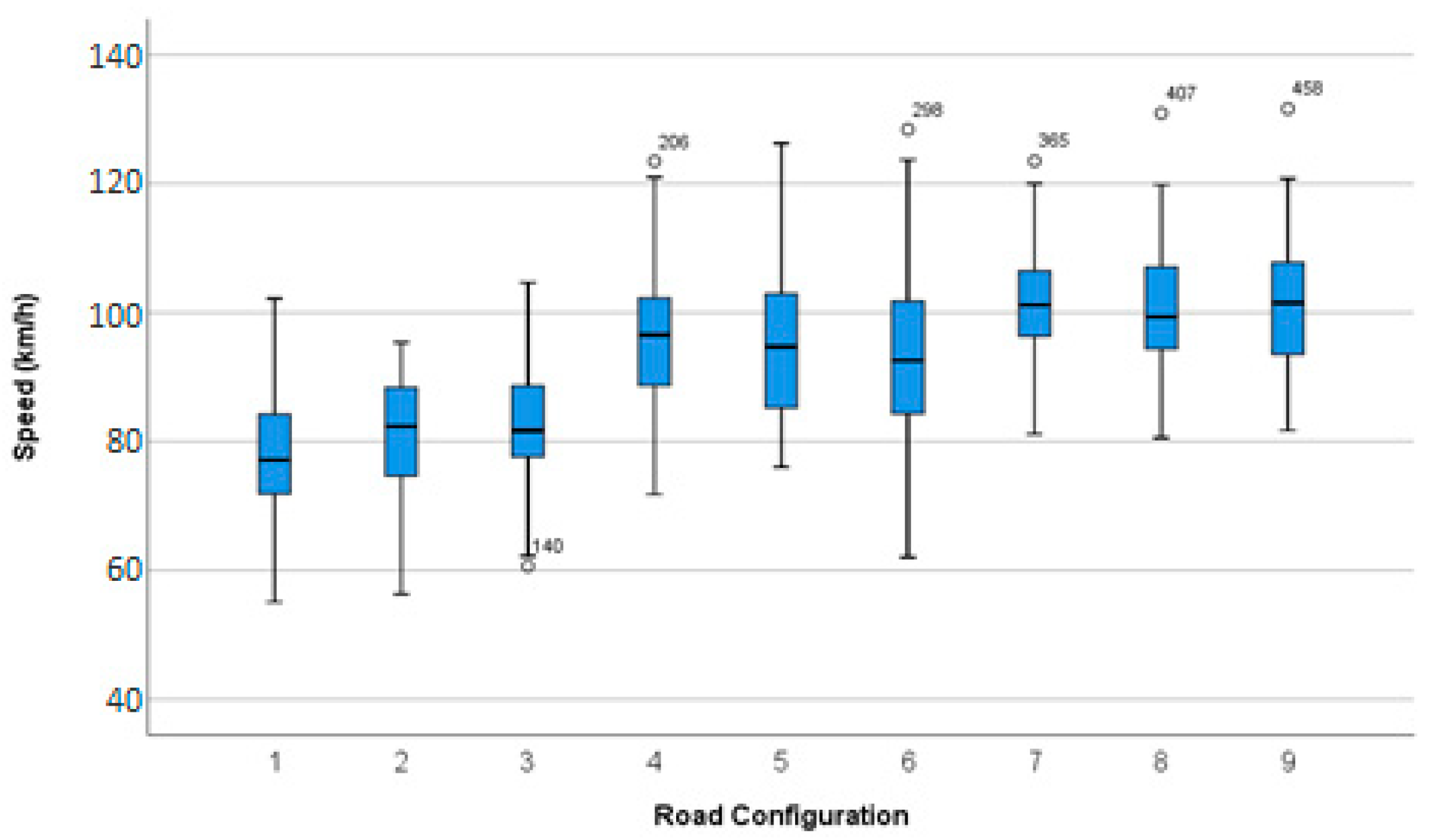
3.1. Driving Speed
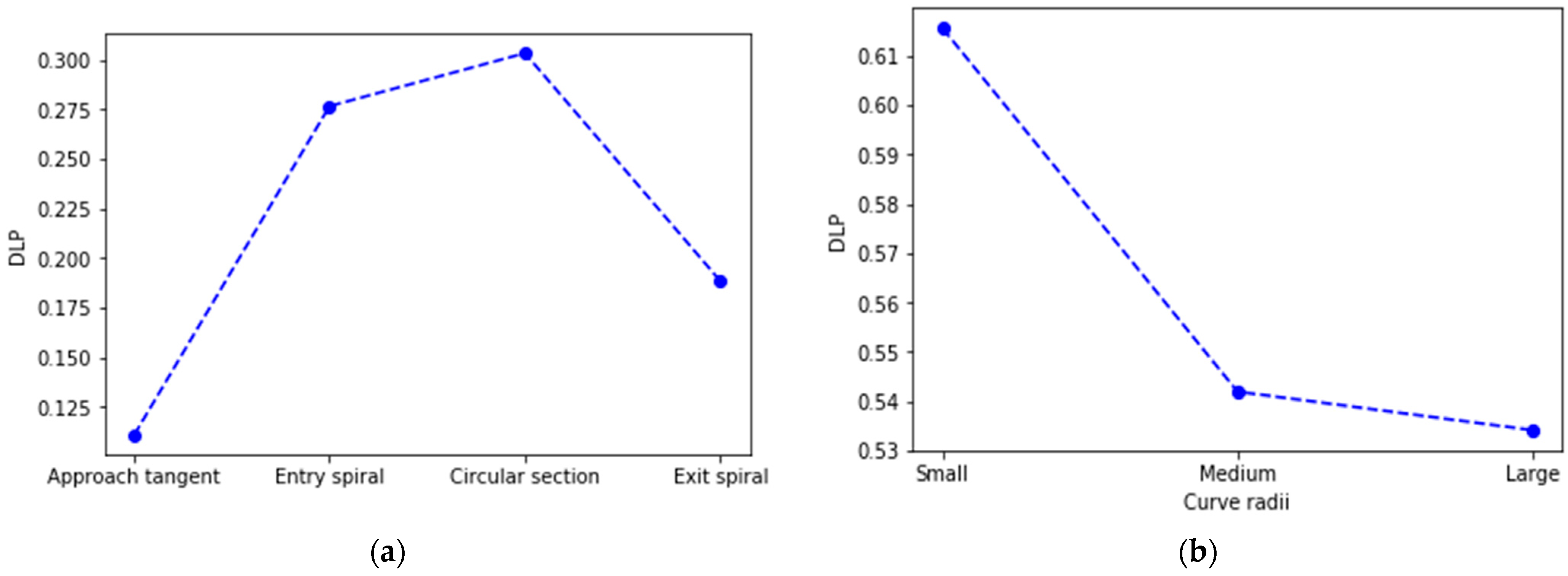
3.2. Lateral Placement
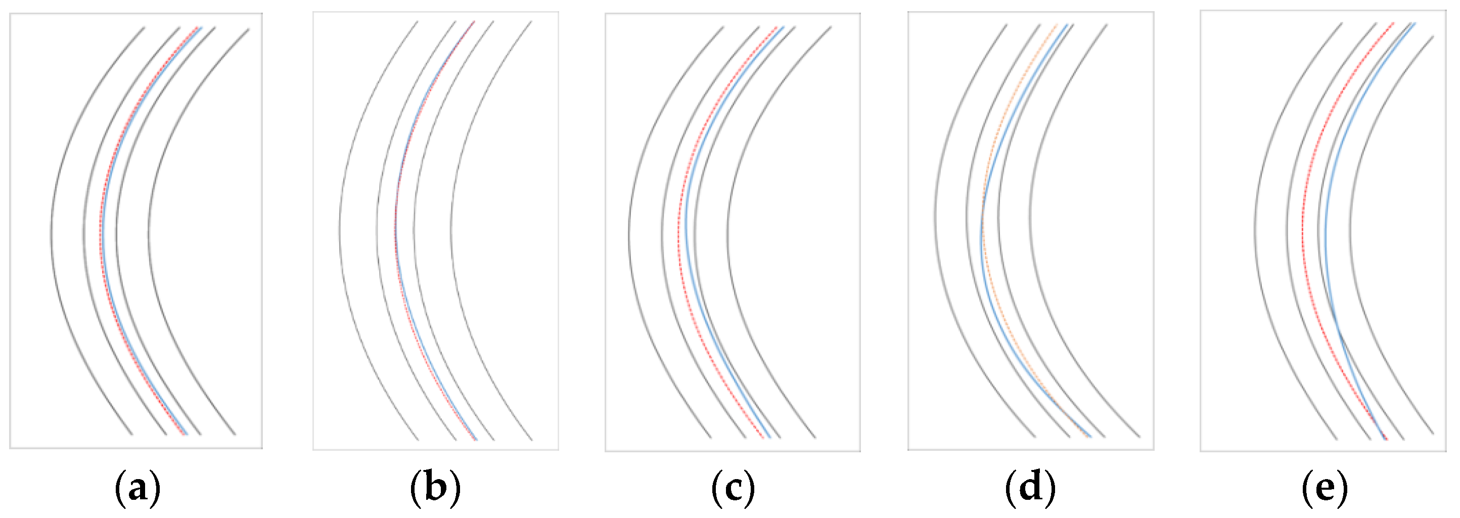
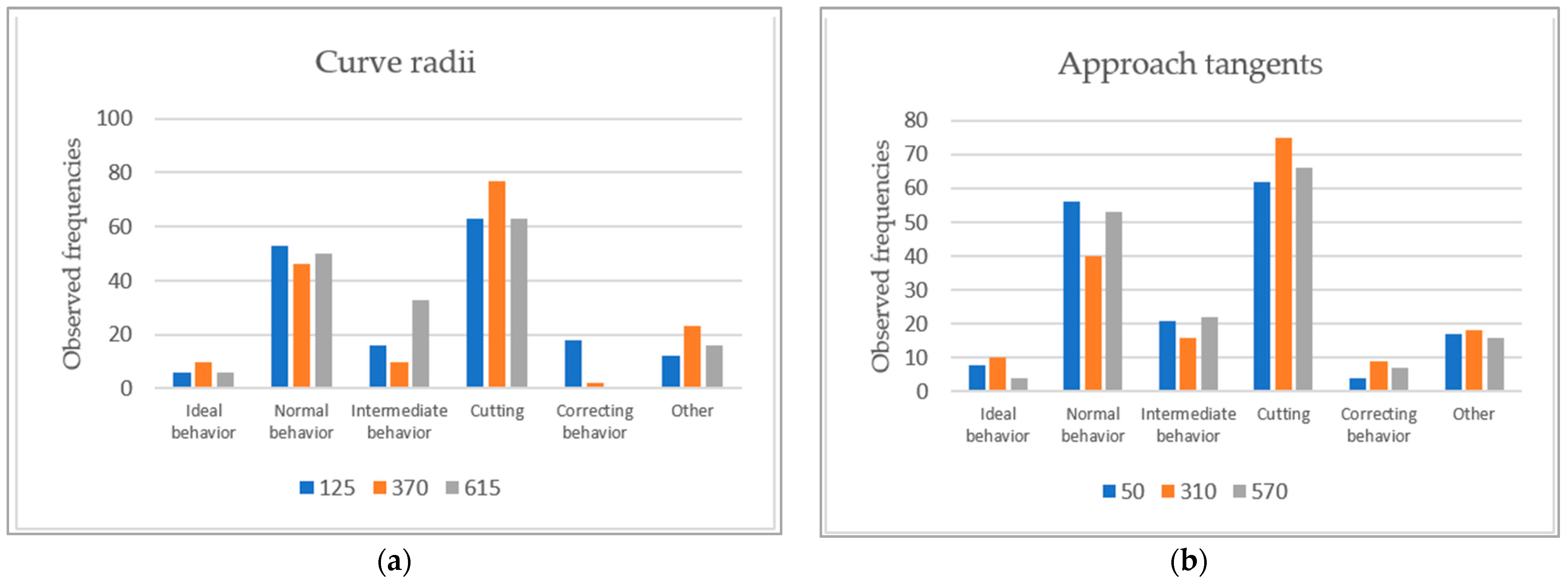
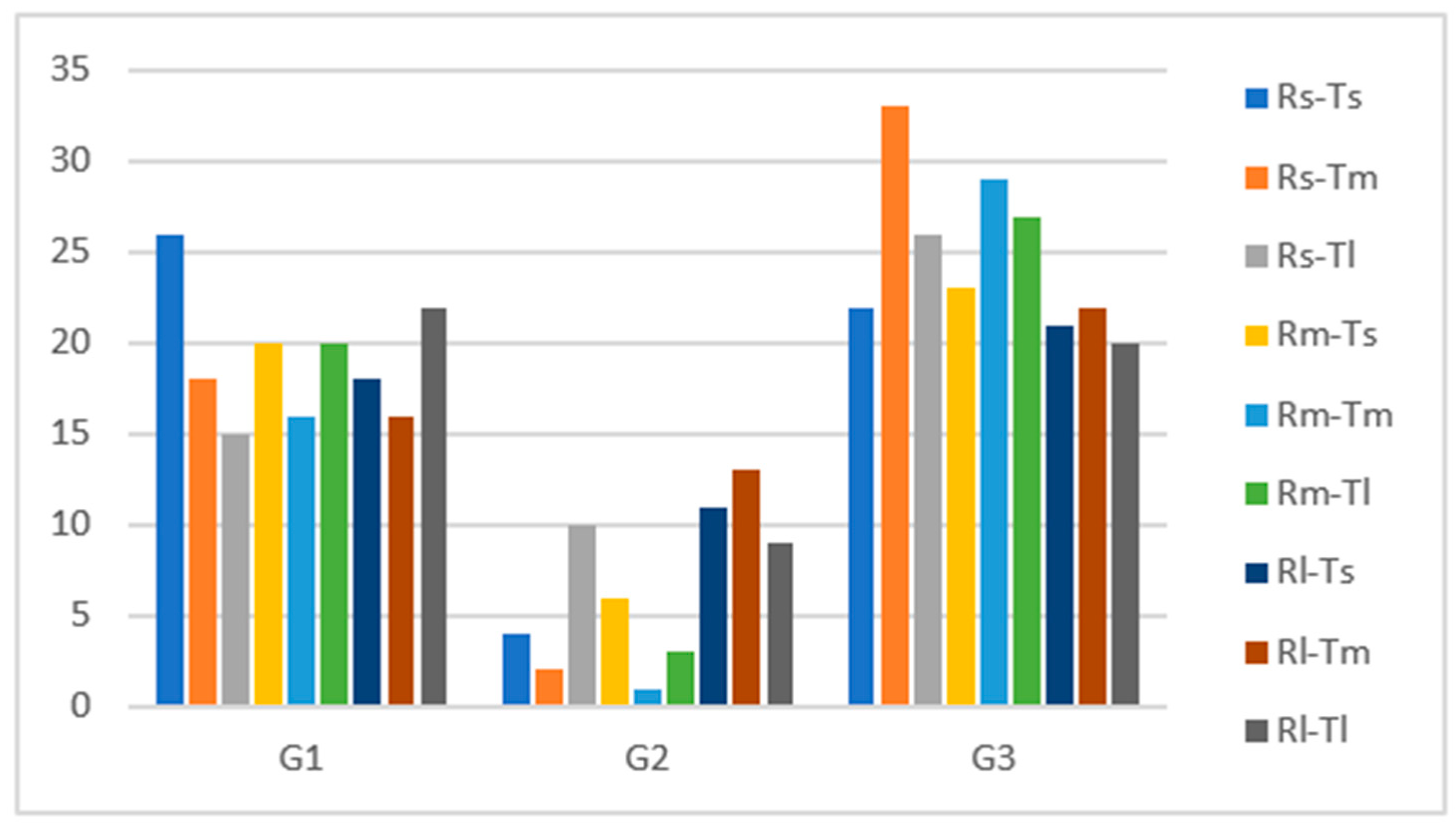
3.3. Driver Classification on Curve Trajectories
3.4. Eye-Movements Data Analysis
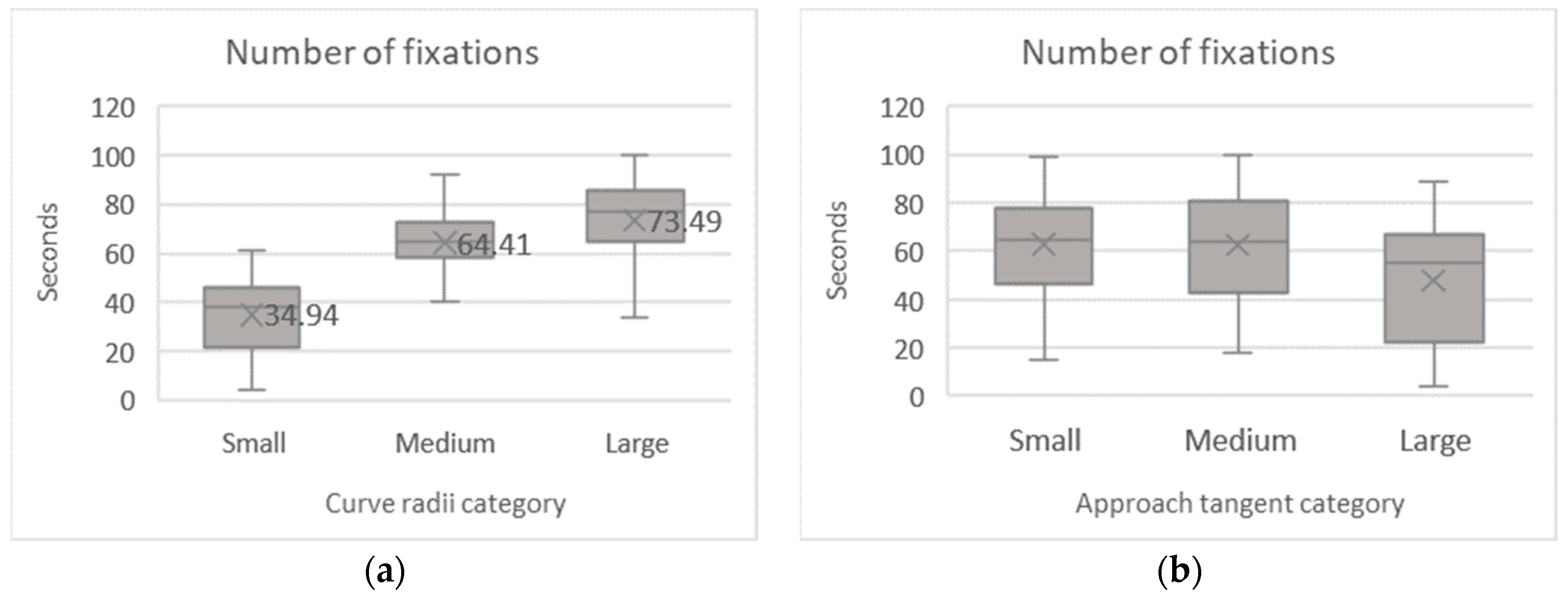
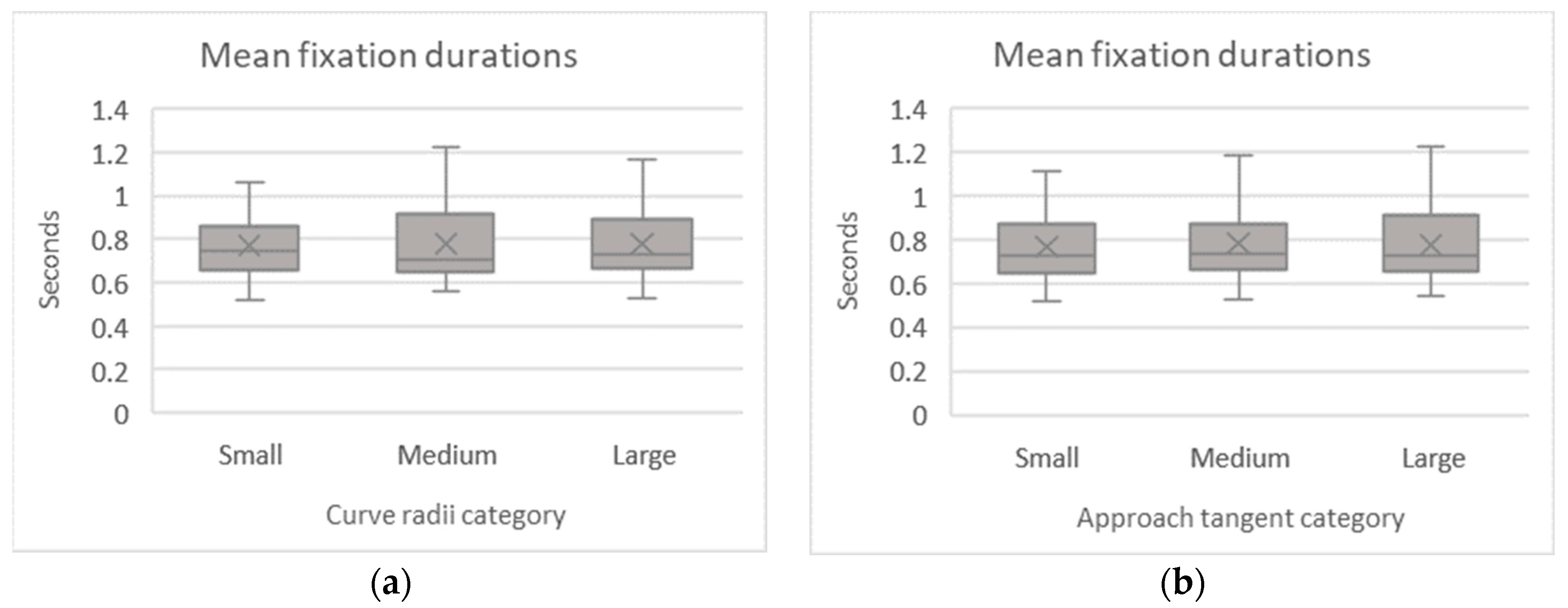
3.4.1. Fixations
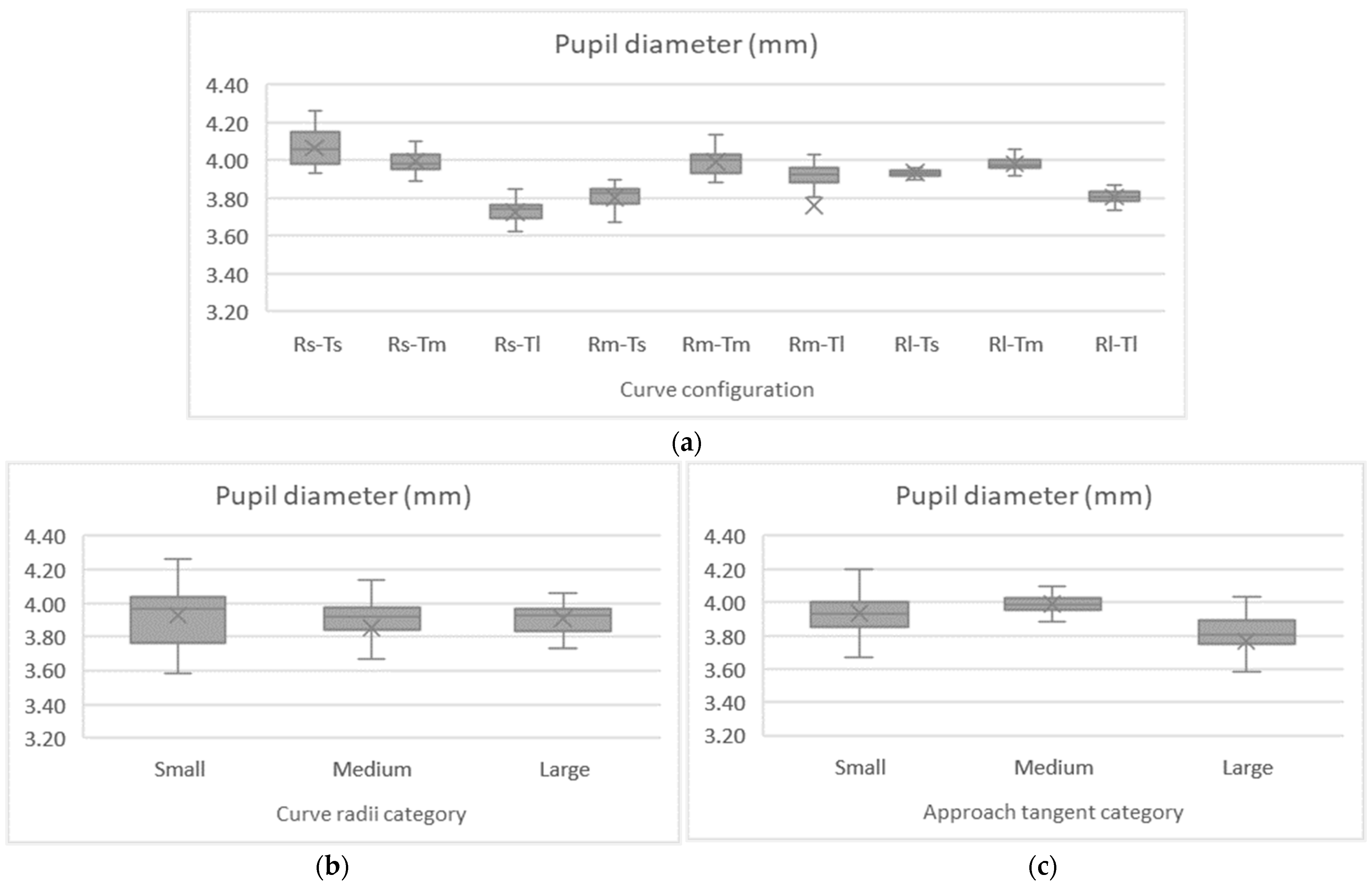
3.4.2. Pupil Diameter Analysis
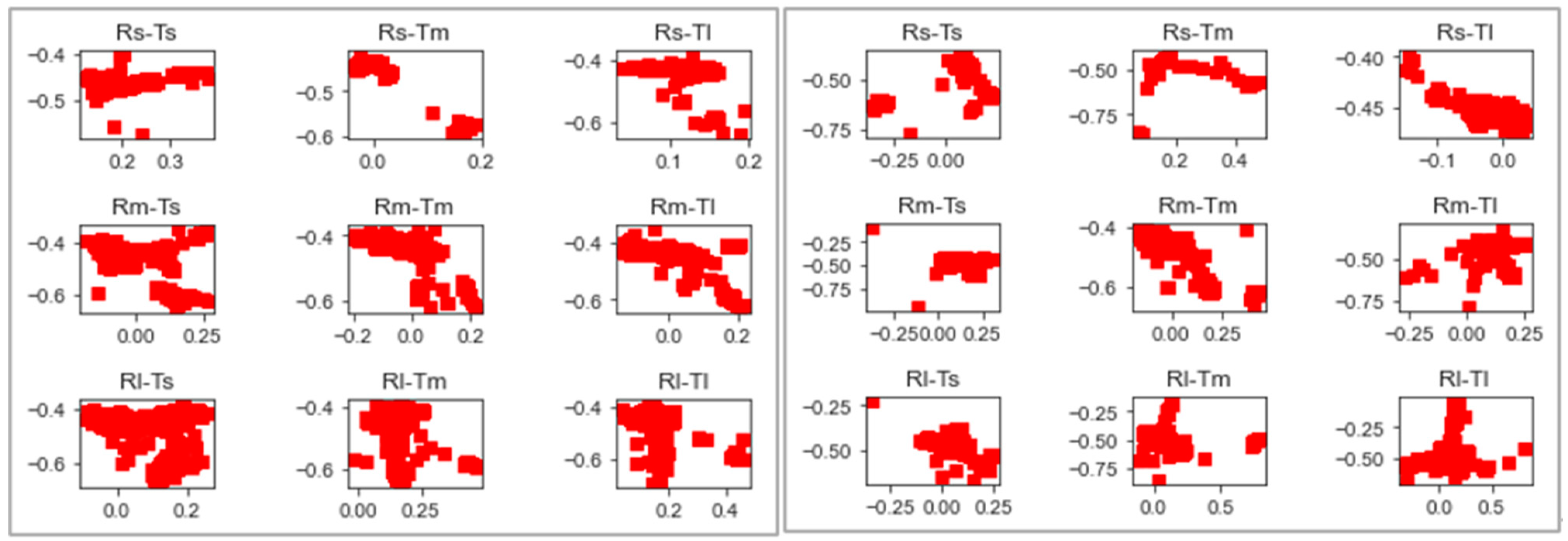
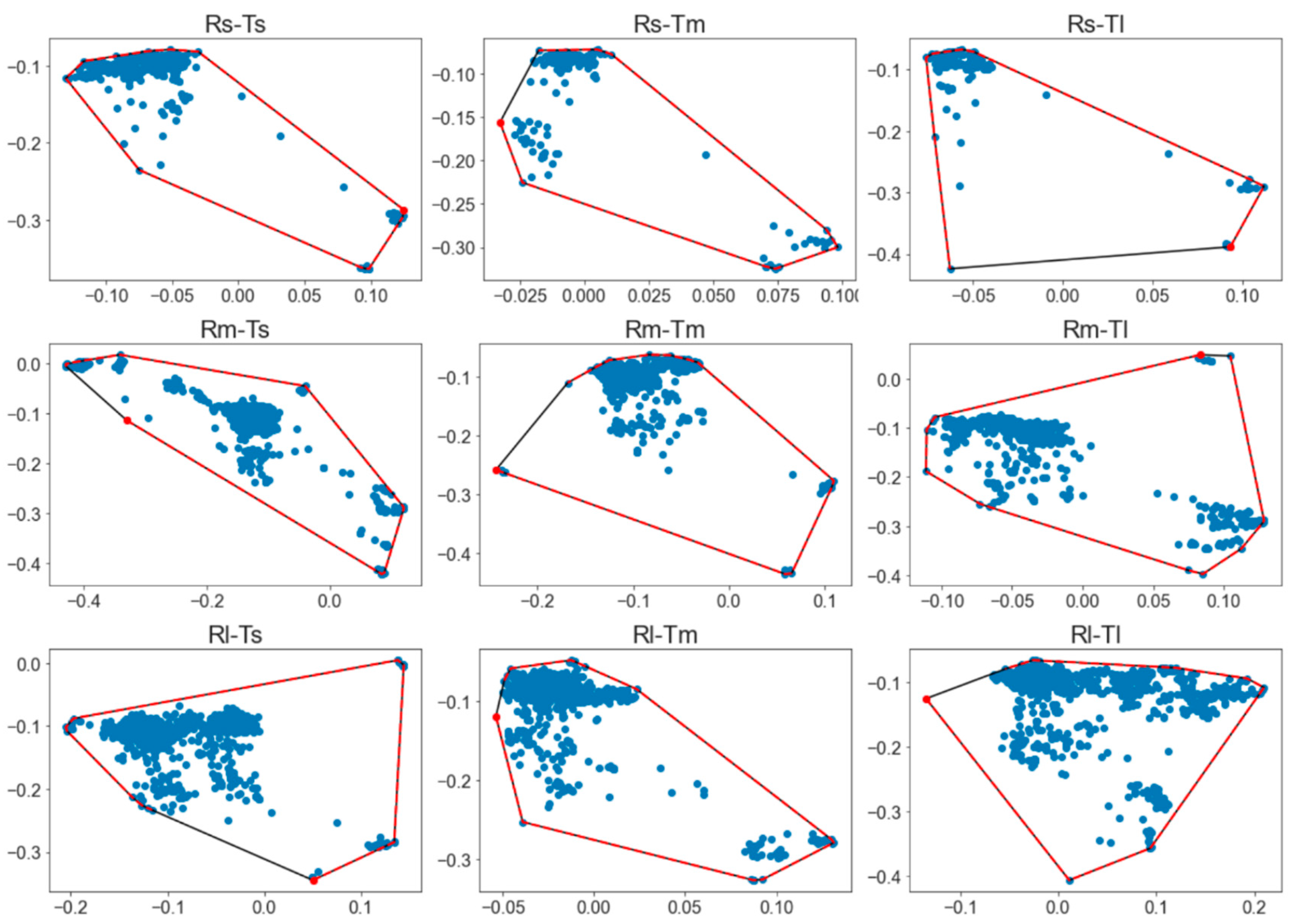
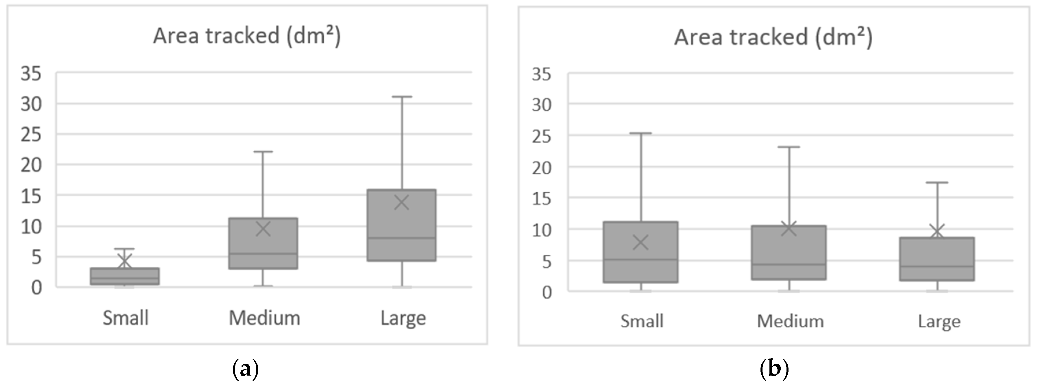
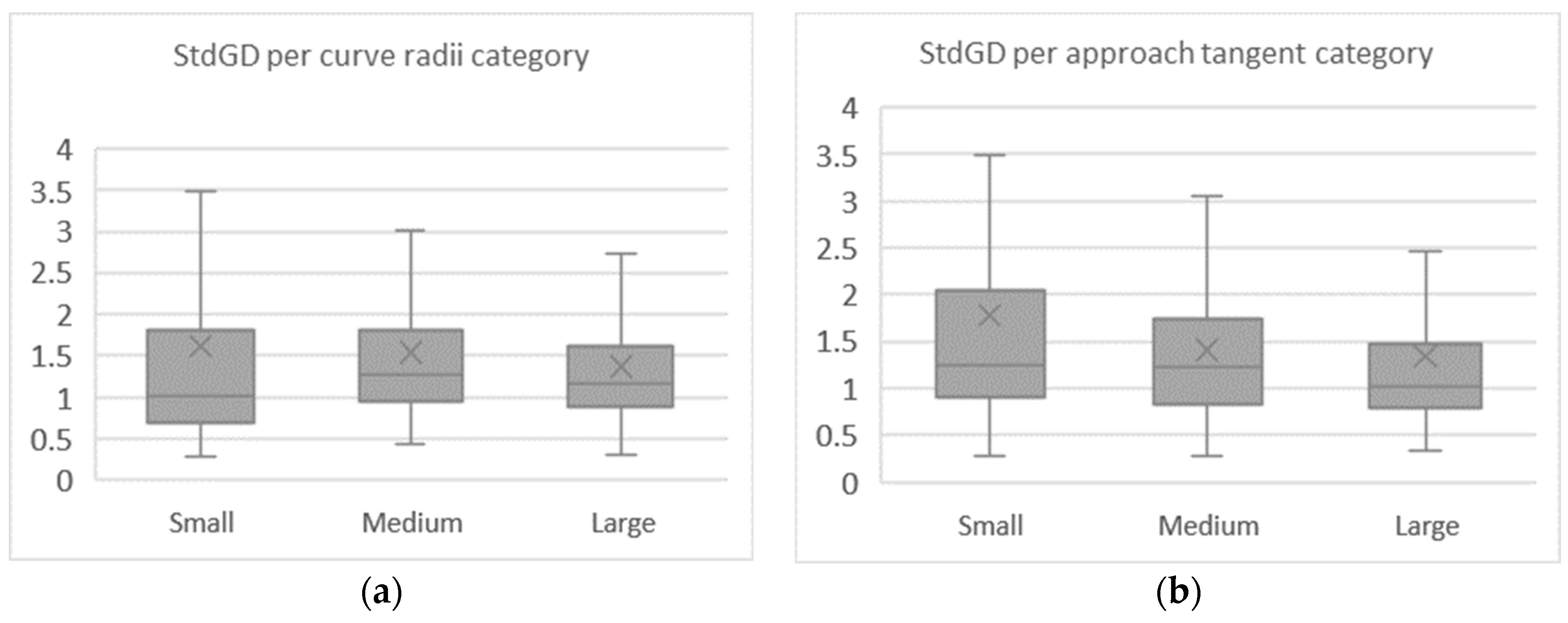
3.4.3. Gaze Analysis
4. Conclusions
Author Contributions
Funding
Institutional Review Board Statement
Informed Consent Statement
Data Availability Statement
Acknowledgments
Conflicts of Interest
References
- Nama, S.; Maurya, A.K.; Maji, A.; Edara, P.; Sahu, P. Vehicle Speed Characteristics and Alignment Design Consistency for Mountainous Roads. Transp. Dev. Econ. 2016, 2, 23. [Google Scholar] [CrossRef] [Green Version]
- Barendswaard, S.; Van Breugel, L.; Schelfaut, B.; Sluijter, J.; Zuiker, L.; Pool, D.M.; Boer, E.R.; Abbink, D. Effect of velocity and curve radius on driver steering behaviour before curve entry. In Proceedings of the 2019 IEEE International Conference on Systems, Man and Cybernetics (SMC), Bari, Italy, 6–9 October 2019; pp. 3866–3871. [Google Scholar] [CrossRef]
- Calvi, A. A Study on Driving Performance Along Horizontal Curves of Rural Roads. J. Transp. Saf. Secur. 2015, 7, 243–267. [Google Scholar] [CrossRef]
- Charly, A.; Mathew, T.V. Evaluation of driving performance in relation to safety on an expressway using field driving data. Transp. Lett. 2020, 12, 340–348. [Google Scholar] [CrossRef]
- Choudhari, T.; Maji, A. Effect of Horizontal Curve Geometry on the Maximum Speed Reduction: A Driving Simulator-Based Study. Transp. Dev. Econ. 2019, 5, 14. [Google Scholar] [CrossRef]
- Hallmark, S.L.; Hawkins, N.; Smadi, O. Relationship Between Speed and Lateral Position On Curves. Accid. Reconstr. J. 2014. Available online: https://rosap.ntl.bts.gov/view/dot/26103 (accessed on 9 April 2022).
- Mauriello, F.; Montella, A.; Pernetti, M.; Galante, F. An Exploratory Analysis of Curve Trajectories on Two-Lane Rural Highways. Sustainability 2018, 10, 4248. [Google Scholar] [CrossRef] [Green Version]
- Sil, G.; Nama, S.; Maji, A.; Maurya, A.K. Effect of horizontal curve geometry on vehicle speed distribution: A four-lane divided highway study. Transp. Lett. 2019, 12, 713–722. [Google Scholar] [CrossRef]
- Suh, W.; Park, P.Y.-J.; Park, C.H.; Chon, K.S. Relationship between Speed, Lateral Placement, and Drivers’ Eye Movement at Two-Lane Rural Highways. J. Transp. Eng. 2006, 132, 649–653. [Google Scholar] [CrossRef]
- Wang, X.; Wang, X. Speed change behavior on combined horizontal and vertical curves: Driving simulator-based analysis. Accid. Anal. Prev. 2018, 119, 215–224. [Google Scholar] [CrossRef]
- Charlton, S.G. The role of attention in horizontal curves: A comparison of advance warning, delineation, and road marking treatments. Accid. Anal. Prev. 2007, 39, 873–885. [Google Scholar] [CrossRef]
- Llopis-Castelló, D.; Bella, F.; Camacho-Torregrosa, F.J.; García, A. New Consistency Model Based on Inertial Operating Speed Profiles for Road Safety Evaluation. J. Transp. Eng. Part A Syst. 2018, 144, 04018006. [Google Scholar] [CrossRef] [Green Version]
- Bassani, M.; Hazoor, A.; Catani, L. What’s around the curve? A driving simulation experiment on compensatory strategies for safe driving along horizontal curves with sight limitations. Transp. Res. Part F Traffic Psychol. Behav. 2019, 66, 273–291. [Google Scholar] [CrossRef]
- Llopis-Castelló, D.; Camacho-Torregrosa, F.J.; Marín-Morales, J.; Pérez-Zuriaga, A.M.; García, A.; Dols, J.F. Validation of a Low-Cost Driving Simulator Based on Continuous Speed Profiles. Transp. Res. Rec. J. Transp. Res. Board 2016, 2602, 104–114. [Google Scholar] [CrossRef] [Green Version]
- Ariën, C.; Brijs, K.; Vanroelen, G.; Ceulemans, W.; Jongen, E.M.M.; Daniels, S.; Brijs, T.; Wets, G. The effect of pavement markings on driving behaviour in curves: A simulator study. Ergonomics 2017, 60, 701–713. [Google Scholar] [CrossRef] [PubMed] [Green Version]
- Awan, H.H.; Pirdavani, A.; Houben, A.; Westhof, S.; Adnan, M.; Brijs, T. Impact of perceptual countermeasures on driving behavior at curves using driving simulator. Traffic Inj. Prev. 2019, 20, 93–99. [Google Scholar] [CrossRef] [PubMed]
- Babić, D.; Fiolić, M.; Gates, T. Road Markings and Their Impact on Driver Behaviour and Road Safety: A Systematic Review of Current Findings. J. Adv. Transp. 2020, 2020, 7843743. [Google Scholar] [CrossRef]
- Charlton, S.G.; Starkey, N.J.; Malhotra, N. Using road markings as a continuous cue for speed choice. Accid. Anal. Prev. 2018, 117, 288–297. [Google Scholar] [CrossRef]
- Babić, D.; Brijs, T. Low-cost road marking measures for increasing safety in horizontal curves: A driving simulator study. Accid. Anal. Prev. 2021, 153, 106013. [Google Scholar] [CrossRef]
- Montella, A.; Galante, F.; Imbriani, L.L.; Mauriello, F.; Pernetti, M. Simulator evaluation of drivers’ behaviour on horizontal curves of two-lane rural highways. Adv. Transp. Stud. 2014, 34, 91–104. [Google Scholar]
- Montella, A.; Galante, F.; Mauriello, F.; Pariota, L. Low-Cost Measures for Reducing Speeds at Curves on Two-Lane Rural Highways. Transp. Res. Rec. J. Transp. Res. Board 2015, 2472, 142–154. [Google Scholar] [CrossRef]
- Wang, X.; Wang, T.; Tarko, A.; Tremont, P.J. The influence of combined alignments on lateral acceleration on mountainous freeways: A driving simulator study. Accid. Anal. Prev. 2015, 76, 110–117. [Google Scholar] [CrossRef]
- Spacek, P. Track Behavior in Curve Areas: Attempt at Typology. J. Transp. Eng. 2005, 131, 669–676. [Google Scholar] [CrossRef]
- Brimley, B.K. Evaluating Unfamiliar Driver Visual Behavior on Horizontal Curves Using Fixation Heat Maps. In Proceedings of the Transportation Research Board 93rd Annual Meeting, Washington, DC, USA, 12–16 January 2014; Volume 14. ISBN 9798459946. [Google Scholar]
- Fitzsimmons, E.J.; Nambisan, S.; Souleyrette, R.R.; Kvam, V. Analyses of Vehicle Trajectories and Speed Profiles Along Horizontal Curves. J. Transp. Saf. Secur. 2013, 5, 187–207. [Google Scholar] [CrossRef]
- Bobermin, M.P.; Silva, M.M.; Ferreira, S. Driving simulators to evaluate road geometric design effects on driver behaviour: A systematic review. Accid. Anal. Prev. 2021, 150, 105923. [Google Scholar] [CrossRef] [PubMed]
- De Ceunynck, T.; Ariën, C.; Brijs, K.; Brijs, T.; Van Vlierden, K.; Kuppens, J.; Van Der Linden, M.; Wets, G. Proactive evaluation of Traffic Signs using a traffic sign simulator. Eur. J. Transp. Infrastruct. Res. 2015, 15, 184–204. [Google Scholar] [CrossRef]
- Larocca, A.P.C.; Ribeiro, R.L.; Figueira, A.D.C.; Oliveira, P.T.M.E.S.D.; Lulio, L.C.; Rangel, M.A.C. Analysis of perception of vertical signaling of highways by drivers in a simulated driving environment. Transp. Res. Part F Traffic Psychol. Behav. 2018, 58, 471–487. [Google Scholar] [CrossRef]
- Hamdar, S.H.; Qin, L.; Talebpour, A. Weather and road geometry impact on longitudinal driving behavior: Exploratory analysis using an empirically supported acceleration modeling framework. Transp. Res. Part C Emerg. Technol. 2016, 67, 193–213. [Google Scholar] [CrossRef] [Green Version]
- Vetturi, D.; Tiboni, M.; Maternini, G.; Bonera, M. Use of eye tracking device to evaluate the driver’s behaviour and the infrastructures quality in relation to road safety. Transp. Res. Procedia 2020, 45, 587–595. [Google Scholar] [CrossRef]
- Gao, K.; Tu, H.; Sun, L.; Sze, N.; Song, Z.; Shi, H. Impacts of reduced visibility under hazy weather condition on collision risk and car-following behavior: Implications for traffic control and management. Int. J. Sustain. Transp. 2019, 14, 635–642. [Google Scholar] [CrossRef]
- Li, X.; Yan, X.; Wong, S. Effects of fog, driver experience and gender on driving behavior on S-curved road segments. Accid. Anal. Prev. 2015, 77, 91–104. [Google Scholar] [CrossRef] [Green Version]
- Cassarino, M.; Maisto, M.; Esposito, Y.; Guerrero, D.; Chan, J.S.; Setti, A. Testing Attention Restoration in a Virtual Reality Driving Simulator. Front. Psychol. 2019, 10, 250. [Google Scholar] [CrossRef]
- Vieira, F.S.; Larocca, A.P.C. Drivers’ speed profile at curves under distraction task. Transp. Res. Part F Traffic Psychol. Behav. 2017, 44, 12–19. [Google Scholar] [CrossRef]
- Farahmand, B.; Boroujerdian, A.M. Effect of road geometry on driver fatigue in monotonous environments: A simulator study. Transp. Res. Part F Traffic Psychol. Behav. 2018, 58, 640–651. [Google Scholar] [CrossRef]
- Xu, J.; Min, J.; Hu, J. Real-time eye tracking for the assessment of driver fatigue. Healthc. Technol. Lett. 2018, 5, 54–58. [Google Scholar] [CrossRef] [PubMed]
- van Huysduynen, H.H.; Terken, J.; Eggen, B. The relation between self-reported driving style and driving behaviour. A simulator study. Transp. Res. Part F Traffic Psychol. Behav. 2018, 56, 245–255. [Google Scholar] [CrossRef]
- Hussain, Q.; Alhajyaseen, W.K.; Pirdavani, A.; Reinolsmann, N.; Brijs, K.; Brijs, T. Speed perception and actual speed in a driving simulator and real-world: A validation study. Transp. Res. Part F Traffic Psychol. Behav. 2019, 62, 637–650. [Google Scholar] [CrossRef]
- Campbell, J.L.; Lichty, M.G.; Brown, J.L.; Richard, C.M.; Graving, J.S.; Graham, J.; O’Laughlin, M.; Torbic, D.; Harwood, D. National Academies of Sciences, Engineering, and Medicine. In Human Factors Guidelines for Road Systems: Second Edition; The National Academies Press: Washington, DC, USA, 2012. [Google Scholar] [CrossRef]
- OpenSCENARIO, version 1.4; VIRES Simulationstechnologie GmbH: Bad Aibling, Germany, 2018.
- Smart Eye Recorder; Version Pro 5.10; Smart Eye AB: Första Långgatan 28B 413 27, Gothenburg, Sweden, 2020.
- De Torquato, T.L.L. Jerk Como Indicador de Consistência Geométrica Para Rodovias; Universidade de São Paulo: São Paulo, Brazil, 2019. [Google Scholar]
- IBM Corp. IBM SPSS Statistics for Windows, version 24.0; IBM Corp.: Armonk, NY, USA, 2016. [Google Scholar]
- Field, A. Descobrindo a Estatística Com SPSS; Artmed: Porto Alegre, Brazil, 2011. [Google Scholar]
- Papadimitriou, E.; Filtness, A.; Theofilatos, A.; Ziakopoulos, A.; Quigley, C.; Yannis, G. Review and ranking of crash risk factors related to the road infrastructure. Accid. Anal. Prev. 2019, 125, 85–97. [Google Scholar] [CrossRef] [Green Version]
- Kolekar, S.; De Winter, J.; Abbink, D. Human-like driving behaviour emerges from a risk-based driver model. Nat. Commun. 2020, 11, 4850. [Google Scholar] [CrossRef]


| Treatments | Length (m) | Deflection Angle (Degrees) | Radius (m) | Approach Tangent (m) | Number of Observations |
|---|---|---|---|---|---|
| Rs-Ts | 182.17 | 56 | 125 | 50 | 56 |
| Rs-Tm | 421.63 | 56 | 125 | 310 | 56 |
| Rs-Tl | 661.09 | 56 | 125 | 570 | 56 |
| Rm-Ts | 182.17 | 56 | 370 | 50 | 56 |
| Rm-Tm | 421.63 | 56 | 370 | 310 | 56 |
| Rm-Tl | 661.09 | 56 | 370 | 570 | 56 |
| Rl-Ts | 182.17 | 56 | 615 | 50 | 56 |
| Rl-Tm | 421.63 | 56 | 615 | 310 | 56 |
| Rl-Tl | 661.09 | 56 | 615 | 570 | 56 |
| Total | 504 |
| Curve Configuration | Radius (m) | Approach Tangent (m) | Speed (km/h) | K–S | ||
|---|---|---|---|---|---|---|
| Average | SD | p-Value | ||||
| 1 | Rs-Ts | 125 | 50 | 77.10 | 1.38 | 0.20 |
| 2 | Rs-Tm | 125 | 310 | 80.79 | 1.34 | 0.20 |
| 3 | Rs-Tl | 125 | 570 | 82.93 | 1.31 | 0.03 * |
| 4 | Rm-Ts | 370 | 50 | 96.05 | 1.61 | 0.20 |
| 5 | Rm-Tm | 370 | 310 | 96.06 | 1.79 | 0.20 |
| 6 | Rm-Tl | 370 | 570 | 94.00 | 1.83 | 0.20 |
| 7 | Rl-Ts | 615 | 50 | 101.03 | 1.41 | 0.20 |
| 8 | Rl-Tm | 615 | 310 | 100.48 | 1.54 | 0.20 |
| 9 | Rl-Tl | 615 | 570 | 101.22 | 1.52 | 0.20 |
| Curve Configuration | Speed Change Behavior | |||||
|---|---|---|---|---|---|---|
| SSD | SS | SSI | ||||
| Rs-Ts | 32 | (61.54%) | 16 | (30.77%) | 4 | (7.69%) |
| Rs-Tm | 44 | (83.02%) | 4 | (7.55%) | 5 | (9.43%) |
| Rs-Tl | 48 | (94.12%) | 2 | (3.92%) | 1 | (1.96%) |
| Rm-Ts | 22 | (44.90%) | 13 | (26.53%) | 14 | (28.57%) |
| Rm-Tm | 29 | (63.04%) | 9 | (19.57%) | 8 | (17.39%) |
| Rm-Tl | 40 | (80.00%) | 8 | (16.00%) | 2 | (4.00%) |
| Rl-Ts | 14 | (28.00%) | 16 | (32.00%) | 20 | (40.00%) |
| Rl-Tm | 16 | (31.37%) | 11 | (21.57%) | 24 | (47.06%) |
| Rl-Tl | 31 | (60.78%) | 11 | (21.57%) | 9 | (17.65%) |
| Total | 276 | (60.93%) | 90 | (19.87%) | 87 | (19.21%) |
| Curve Configuration | Radius (m) | Approach Tangent (m) | DLP (m) | K–S | ||
|---|---|---|---|---|---|---|
| Average | SD | p-Value | ||||
| 1 | Rs-Ts | 125 | 50 | 0.20 | 0.13 | 0.015 * |
| 2 | Rs-Tm | 125 | 310 | 0.32 | 0.22 | 0.013 * |
| 3 | Rs-Tl | 125 | 570 | 0.32 | 0.22 | 0.006 ** |
| 4 | Rm-Ts | 370 | 50 | 0.27 | 0.20 | 0.000 *** |
| 5 | Rm-Tm | 370 | 310 | 0.34 | 0.31 | 0.000 *** |
| 6 | Rm-Tl | 370 | 570 | 0.29 | 0.25 | 0.000 *** |
| 7 | Rl-Ts | 615 | 50 | 0.30 | 0.21 | 0.000 *** |
| 8 | Rl-Tm | 615 | 310 | 0.35 | 0.34 | 0.000 *** |
| 9 | Rl-Tl | 615 | 570 | 0.33 | 0.25 | 0.000 *** |
| Class | Approach Tangent | Curve | Total | |
|---|---|---|---|---|
| 1. Ideal behavior | |LP|max ≤ 0.65 or 2.95 ≤ |LP|max ≤ 4.25 | |LP|max ≤ 0.55 or 3.05 ≤ |LP|max ≤ 4.15 | ||
| 2. Normal behavior | |LP|max ≤ 0.9 or 2.7 ≤ |LP|max ≤ 4.5 |∆LP|max ≤ 1.2 | |LP|max ≤ 0.9 or 2.7 ≤ |LP|max ≤ 4.5 |∆LP|max ≤ 1.2 | ||
| 3. Intermediate behavior | 3.1 Driving close to the centerline | |LP|max ≤ 1.0 or 2.6 ≤ |LP|max ≤ 4.6 |∆LP|max ≤ 1.1 | LPmean > 0.5 | |
| 3.2 Driving outside in curve approach | 1.0 < |LP|max < 2.6 or |LP|max > 4.6 | |LP|max ≤ 1.0 or 2.6 ≤ |LP|max ≤ 4.5 LPmean ≤ 0.5 | ||
| 4. Cutting | 4.1 Right curves | |||
| lane 1 | LPmin < −3.70 | LPmax > −3.2 | ||
| lane 2 | LPmin < −0.10 | LPmax > 0.40 | ||
| lane 3 | LPmin < 3.50 | LPmax > 4.00 | ||
| 4.2 Left curves | ||||
| lane 1 | LPmax > −3.50 | LPmin < −4.00 | ||
| lane 2 | LPmax > 0.10 | LPmin < -0.40 | ||
| lane 3 | LPmax > 3.70 | LPmin < 3.20 | ||
| 5. Correcting behavior | 5.1 in approach | alat_max > 4 m/s2 | - | |
| 5.2 on the curve | - | alat_max > 4 m/s2 | ||
| 5.3 multiple corrections | Combination of behaviors 5.1 and 5.2 | |||
| Behavior | Ts | Tm | Tl | Total | ||||||||
|---|---|---|---|---|---|---|---|---|---|---|---|---|
| Rs | Rm | Rl | Rs | Rm | Rl | Rs | Rm | Rl | Rs | Rm | Rl | |
| 1 Ideal behavior | 5.36 | 3.57 | 1.79 | 5.36 | 7.14 | 5.36 | 3.57 | 7.14 | 0.00 | 3.57 | 5.95 | 3.57 |
| 2 Normal behavior | 41.07 | 28.57 | 25.00 | 30.36 | 21.43 | 30.36 | 28.57 | 21.43 | 39.29 | 31.55 | 27.38 | 29.76 |
| 3 Intermediate behavior | 7.14 | 3.57 | 17.86 | 10.71 | 1.79 | 5.36 | 19.64 | 23.21 | 16.07 | 9.52 | 5.95 | 19.64 |
| 4 Cutting | 32.14 | 44.64 | 35.71 | 41.07 | 50.00 | 46.43 | 37.50 | 39.29 | 35.71 | 37.50 | 45.83 | 37.50 |
| 5 Correcting behavior | 7.14 | 14.29 | 10.71 | 0.00 | 1.79 | 1.79 | 0.00 | 0.00 | 0.00 | 10.71 | 1.19 | 0.00 |
| 6 Others | 7.14 | 5.36 | 8.93 | 12.50 | 17.86 | 10.71 | 10.71 | 8.93 | 8.93 | 7.14 | 13.69 | 9.52 |
| Total | 100 | 100 | 100 | 100 | 100 | 100 | 100 | 100 | 100 | 100 | 100 | 100 |
| Curve Configuration | Radius (m) | Approach Tangent (m) | Number of Fixations | K–S | ||
|---|---|---|---|---|---|---|
| Average | SD | p-Value | ||||
| 1 | Rs-Ts | 125 | 50 | 44.34 | 10.87 | 0.077 |
| 2 | Rs-Tm | 125 | 310 | 41.22 | 9.01 | 0.126 |
| 3 | Rs-Tl | 125 | 570 | 19.26 | 4.99 | 0.002 ** |
| 4 | Rm-Ts | 370 | 50 | 64.39 | 12.04 | 0.000 *** |
| 5 | Rm-Tm | 370 | 310 | 71.39 | 14.98 | 0.000 *** |
| 6 | Rm-Tl | 370 | 570 | 57.43 | 11.57 | 0.000 *** |
| 7 | Rl-Ts | 615 | 50 | 79.65 | 16.44 | 0.000 *** |
| 8 | Rl-Tm | 615 | 310 | 74.34 | 18.44 | 0.000 *** |
| 9 | Rl-Tl | 615 | 570 | 66.48 | 15.80 | 0.000 *** |
| Curve Configuration | Radius (m) | Approach Tangent (m) | Fixation Duration (s) | K–S | ||
|---|---|---|---|---|---|---|
| Average | SD | p-Value | ||||
| 1 | Rs-Ts | 125 | 50 | 0.752 | 0.137 | 0.200 |
| 2 | Rs-Tm | 125 | 310 | 0.764 | 0.146 | 0.000 *** |
| 3 | Rs-Tl | 125 | 570 | 0.793 | 0.152 | 0.011 * |
| 4 | Rm-Ts | 370 | 50 | 0.778 | 0.171 | 0.003 ** |
| 5 | Rm-Tm | 370 | 310 | 0.792 | 0.198 | 0.011 * |
| 6 | Rm-Tl | 370 | 570 | 0.767 | 0.169 | 0.021 * |
| 7 | Rl-Ts | 615 | 50 | 0.773 | 0.142 | 0.000 *** |
| 8 | Rl-Tm | 615 | 310 | 0.796 | 0.166 | 0.002 ** |
| 9 | Rl-Tl | 615 | 570 | 0.772 | 0.162 | 0.000 * |
| Curve Configuration | Radius (m) | Approach Tangent (m) | Pupil Diameter (cm) | K–S | ||
|---|---|---|---|---|---|---|
| Average | SD | p-Value | ||||
| 1 | Rs-Ts | 125 | 50 | 0.418 | 0.023 | 0.200 |
| 2 | Rs-Tm | 125 | 310 | 0.403 | 0.018 | 0.005 ** |
| 3 | Rs-Tl | 125 | 570 | 0.382 | 0.011 | 0.004 ** |
| 4 | Rm-Ts | 370 | 50 | 0.363 | 0.018 | 0.000 *** |
| 5 | Rm-Tm | 370 | 310 | 0.407 | 0.011 | 0.200 |
| 6 | Rm-Tl | 370 | 570 | 0.403 | 0.024 | 0.000 *** |
| 7 | Rl-Ts | 615 | 50 | 0.382 | 0.009 | 0.000 *** |
| 8 | Rl-Tm | 615 | 310 | 0.398 | 0.015 | 0.005 ** |
| 9 | Rl-Tl | 615 | 570 | 0.393 | 0.027 | 0.000 *** |
| Curve Configuration | Radius (m) | Approach Tangent (m) | Area (m2) | K–S | ||
|---|---|---|---|---|---|---|
| Average | SD | p-Value | ||||
| 1 | Rs-Ts | 125 | 50 | 0.030 | 0.033 | 0.000 *** |
| 2 | Rs-Tm | 125 | 310 | 0.040 | 0.073 | 0.000 *** |
| 3 | Rs-Tl | 125 | 570 | 0.056 | 0.241 | 0.000 *** |
| 4 | Rm-Ts | 370 | 50 | 0.090 | 0.087 | 0.007 ** |
| 5 | Rm-Tm | 370 | 310 | 0.091 | 0.113 | 0.000 *** |
| 6 | Rm-Tl | 370 | 570 | 0.121 | 0.192 | 0.000 *** |
| 7 | Rl-Ts | 615 | 50 | 0.126 | 0.136 | 0.000 *** |
| 8 | Rl-Tm | 615 | 310 | 0.167 | 0.316 | 0.000 *** |
| 9 | Rl-Tl | 615 | 570 | 0.124 | 0.147 | 0.000 *** |
| Curve Configuration | Radius (m) | Approach Tangent (m) | StdGD | K–S | ||
|---|---|---|---|---|---|---|
| Average | SD | p-Value | ||||
| 1 | Rs-Ts | 125 | 50 | 2.07 | 3.60 | 0.000 *** |
| 2 | Rs-Tm | 125 | 310 | 1.42 | 0.92 | 0.000 *** |
| 3 | Rs-Tl | 125 | 570 | 1.36 | 1.02 | 0.000 *** |
| 4 | Rm-Ts | 370 | 50 | 1.69 | 0.87 | 0.023 * |
| 5 | Rm-Tm | 370 | 310 | 1.41 | 0.65 | 0.004 ** |
| 6 | Rm-Tl | 370 | 570 | 1.51 | 1.31 | 0.000 *** |
| 7 | Rl-Ts | 615 | 50 | 1.56 | 0.81 | 0.009 ** |
| 8 | Rl-Tm | 615 | 310 | 1.39 | 0.75 | 0.045 * |
| 9 | Rl-Tl | 615 | 570 | 1.13 | 0.59 | 0.000 *** |
Publisher’s Note: MDPI stays neutral with regard to jurisdictional claims in published maps and institutional affiliations. |
© 2022 by the authors. Licensee MDPI, Basel, Switzerland. This article is an open access article distributed under the terms and conditions of the Creative Commons Attribution (CC BY) license (https://creativecommons.org/licenses/by/4.0/).
Share and Cite
Rondora, M.E.S.; Pirdavani, A.; Larocca, A.P.C. Driver Behavioral Classification on Curves Based on the Relationship between Speed, Trajectories, and Eye Movements: A Driving Simulator Study. Sustainability 2022, 14, 6241. https://0-doi-org.brum.beds.ac.uk/10.3390/su14106241
Rondora MES, Pirdavani A, Larocca APC. Driver Behavioral Classification on Curves Based on the Relationship between Speed, Trajectories, and Eye Movements: A Driving Simulator Study. Sustainability. 2022; 14(10):6241. https://0-doi-org.brum.beds.ac.uk/10.3390/su14106241
Chicago/Turabian StyleRondora, Maria Emilia Schio, Ali Pirdavani, and Ana Paula C. Larocca. 2022. "Driver Behavioral Classification on Curves Based on the Relationship between Speed, Trajectories, and Eye Movements: A Driving Simulator Study" Sustainability 14, no. 10: 6241. https://0-doi-org.brum.beds.ac.uk/10.3390/su14106241