Article

Short-Term Traffic Speed Forecasting Model for a Parallel Multi-Lane Arterial Road Using GPS-Monitored Data Based on Deep Learning Approach

1
Faculty of Civil Engineering, University of Transport and Communications, 3 Cau Giay Rd., Lang Thuong, Dong Da, Hanoi 10000, Vietnam
2
Geographic Information Systems Research Center, Feng Chia University, 100 Wenhua Rd., Situn, Taichung 40724, Taiwan
3
Institute of Techniques for Special Engineering, Le Quy Don Technical University, 236 Hoang Quoc Viet Rd., Co Nhue, Bac Tu Liem, Hanoi 10000, Vietnam
*
Author to whom correspondence should be addressed.
Sustainability 2022, 14(10), 6351; https://0-doi-org.brum.beds.ac.uk/10.3390/su14106351
Submission received: 15 April 2022 / Revised: 15 May 2022 / Accepted: 20 May 2022 / Published: 23 May 2022
(This article belongs to the Special Issue Transportation Safety and Pavement Management)

Abstract

:
Traffic speed forecasting in the short term is one of the most critical parts of any intelligent transportation system (ITS). Accurate speed forecasting can support travelers’ route choices, traffic guidance, and traffic control. This study proposes a deep learning approach using long short-term memory (LSTM) network with tuning hyper-parameters to forecast short-term traffic speed on an arterial parallel multi-lane road in a developing country such as Vietnam. The challenge of mishandling the location data of vehicles on small and adjacent multi-lane roads will be addressed in this study. To test the accuracy of the proposed forecasting model, its application is illustrated using historical voyage GPS-monitored data on the Le Hong Phong urban arterial road in Haiphong city of Vietnam. The results indicate that in comparison with other models (e.g., traditional models and convolutional neural network), the best performance in terms of root mean square error (RMSE), mean absolute error (MAE), and median absolute error (MDAE) is obtained by using the proposed model.

1. Introduction

Vehicle speed is an essential indicator of the operation state of roadways [1,2]. Traffic speed forecasting (TSF), especially short-term TSF (less than 30 min [3]), has become necessary in intelligent transportation systems (ITS) [4]. Short-term TSF has been identified as a key task for many applications, such as developing a proactive traffic control system [2], prospective traffic navigation to avoid potential congestion in advance, just-in-time departure recommendation in trip schedule, the construction of ITS [5], and so on. Hence, accurate TSF is important in many applications of the transportation sector.
Spot detectors can readily collect speed datasets of TSF (e.g., inductive loops, video cameras, microwave radars, and so on) and probe vehicle data or floating car data (e.g., global positioning systems (GPS) devices and cellular-base systems). The spot detectors are expensive and primarily only serve intersections or expressways. It is difficult to identify the problematic links in real-time due to the sparse network of spot detectors. While GPS data collected from vehicles provides spatial and temporal patterns of traffic information [6] and has become increasingly popular to provide data for monitoring fleet management services and traffic management systems due to less cost and being constantly accessible in comparison to those spot detectors, the principle of a GPS-based system is to collect traffic data in real time by locating the vehicle via GPS devices over the entire road network. Dataset of location, speed, and direction of trips is sent anonymously to a central processing center. This information is then processed to obtain average speeds or/and travel time of a vehicle fleet or a single probe vehicle through road segments. Although GPS devices are becoming more and more used and affordable, only a limited number of vehicles are equipped with these devices, typically fleet management services (e.g., taxi, bus, truck, etc.) [7], especially in developing countries such as Vietnam, where public transport and commercial smart vehicles are not well-developed. Moreover, the traffic flow is a typical mixed traffic flow with predominantly motorcycles (over 80% of trips in the urban area by motorcycles [8]) without GPS devices. According to Article 14 of the Decree No. 86/2014/ND-CP, dated 10 September 2014, of the Vietnam government on business and transportation business conditions for a car (Decree No. 86), only business vehicles, including passenger vehicles and goods vehicles (e.g., taxis, buses, trucks, and so forth) are required to install GPS devices to store and transmit travel information to transportation business units. This information only is provided for police or inspector as required. Thus far, GPS data have been used to estimate average travel times and speeds along with road segments and road networks [9]. Many well-known commercial applications (such as Google Maps, Waze, CoPilot, Komoot, and others [10]) now rely on GPS signals from road users to give real-time traffic information and optimal routes. When traffic is heavy, these applications automatically alter the route to save time for drivers. To the authors’ knowledge, these applications employ real-time data to identify traffic conditions and suggest the best route at the time rather than providing predictive information for the future. This is because these applications do not exploit historical time-series data. Besides practical applications, there has also been a great deal of research deploying GPS data to predict short-term traffic speed through the principle of time-series forecasting.
Along with the development of information and communication technology, the models of time-series forecasting in general as well as the TSF model in particular have been gradually shifting from traditional statistical models (e.g., autoregressive integrated moving average (ARIMA) [11], seasonal ARIMA, exponential smoothing model) to models using computational intelligence approaches (e.g., support vector regression (SVR), neural networks [5,11], extended short-term memory networks (LSTM) [2,12], and convolutional neural network (CNN)). The practice has shown that computational intelligence approaches are more capable of abnormal data in comparison with those classical statistical models [13]. Hence, computational intelligence approaches are increasingly interested in short-term forecasting problems. The LSTM is a deep learning artificial recurrent neural network that can analyze full data sequences. LSTM has become a trending approach to time-series forecasting due to the model’s capacity to learn large sequences of observations. LSTM provides several advantages, including capturing both long- and short-term seasonalities, such as yearly and weekly patterns. It may accept inputs of various lengths. For forecasting, it might learn the nonlinear relationship. Image processing [14,15], soft sensor modeling [16], energy consumption [17], speech recognition [18,19], sentiment analysis [20], and autonomous systems [21] are just few of the fields where LSTM has been applied. According to the survey [22] on the employment of deep learning algorithms to tackle the velocity prediction problem, LSTM is still the most preferred. Many studies have used hybrid solutions combining LSTM and other algorithms, for example, the idea that combining CNN and LSTM can handle the spatio-temporal of time series. This study, however, indicates that this is not always the case. This combination does not perform more effectively than LSTM alone in many cases. The authors chose LSTM as a deep learning system for speed prediction based on their findings. It is worth noting that for LSTM to perform properly, its hyper-parameters must be tailored to each data type. This study will address this problem.
Though literature review showed that most short-term TSF models using GPS data are done on expressways [2], a few studies are done on urban arterial roads with GPS data of taxi fleets [11,12] or bus fleets. Short-term TSF on urban arterial roads is more complex due to the signalized intersections, non-signalized intersections, entry/exit points, bus stops, and speed enforcement points, and it also requires more extraordinary samples. The previous models were using GPS data, which mainly use a dataset from taxi or bus fleets; in this paper, we exploit GPS-monitored data from a large number of business vehicles (passenger vehicles and goods vehicles) to deliver traffic speed information throughout an urban arterial road in Haiphong city in Vietnam. Traffic speed estimates are deduced from the historical voyage GPS-monitored data from many vehicles (about 2196) equipped with GPS devices. A significant difference between this study and other studies is its handling of parallel multi-lane arterial road data. The signal confusion between lines and handling abnormal data situations are addressed here. The TFS model using such data has not been carried out in developing countries such as Vietnam to the best of our knowledge. Hence, it has great significance in theory as well as in practice. These are the novelty of the proposed approach and its contribution to existing studies.
To sum up, the main contributions are as follows:
  • Proposing a solution for dealing with inaccurate and abnormal GPS data on parallel multi-lane arterial roads in Vietnam;
  • Designing LSTM network and tuning its hyper-parameters to predict traffic speed on the urban arterial road under historical voyage GPS-monitored data;
  • Comparing the proposed method to other standard traffic flow prediction methods. Experiments show that the proposed model outperforms different approaches to traffic speed forecasting.
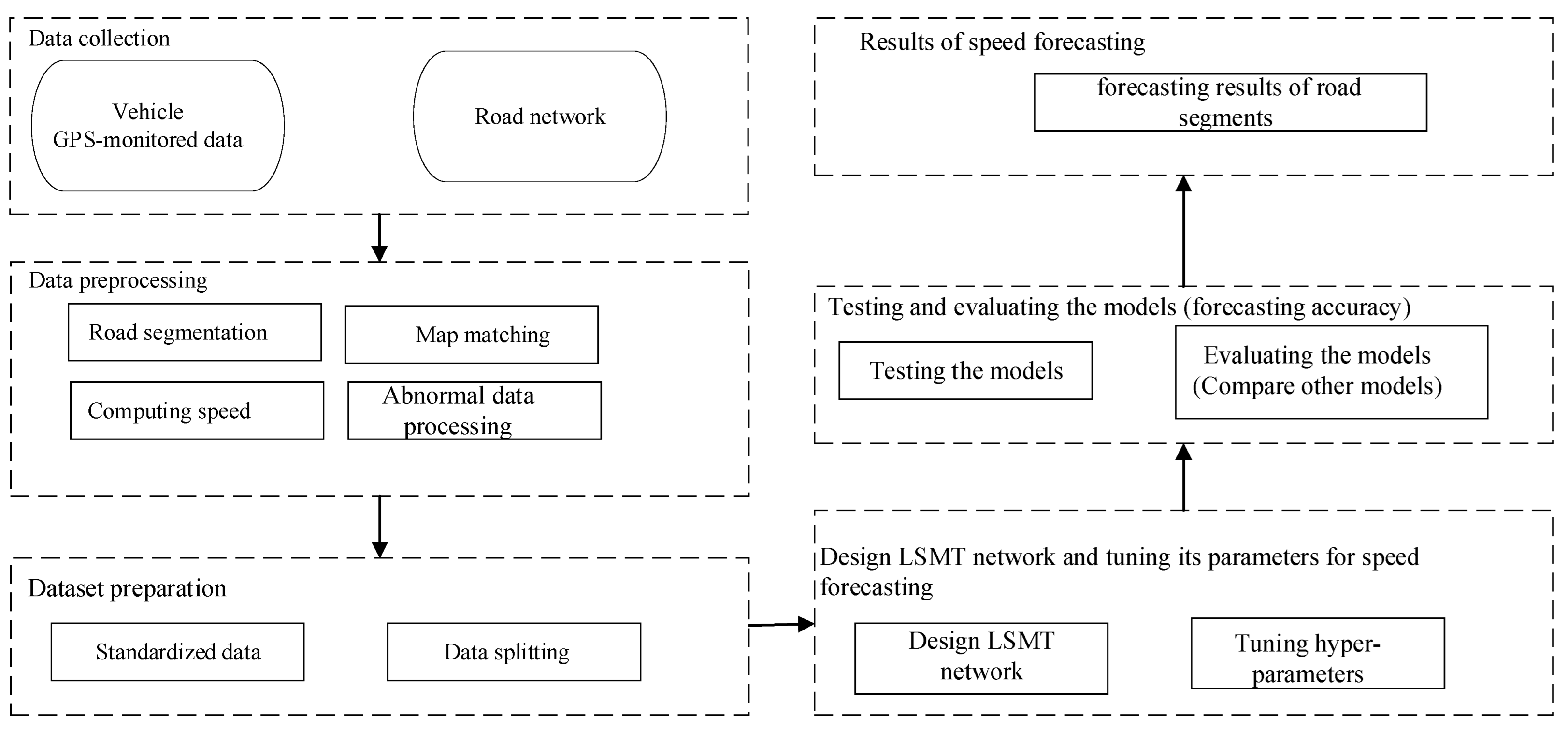
2. Data and Methods

Generally, TSF means to predict the future speed of each road segment based on historical observations [5]. The methodologies of TSF fall into three major categories: parametric approach, nonparametric approach, and deep learning approach [23]. Table 1 summarizes some of these groups’ case studies.

2.1. Parametric Approaches

Many past studies developed various parametric speed and forecast models in which the best models are being adapted for traffic simulator applications [42]. The parametric method has a fixed structure, while the parameters are learned from the dataset [43]. Several models developed for short-term speed and traffic flow forecasting are exponential smoothing (ES) models, autoregressive moving average (ARMA) [24], ARIMA models [25,27], Kohonen–ARIMA [28], seasonal ARIMA [44,45], ARIMA with explanatory variables (ARIMAX) [46], SARIMA-SDGM model [2], and PROPHET [47]. In general, parametric techniques are simple to use and provide a clear theoretical understanding as well as a logical computational framework. However, the bulk of these systems has been shown to perform poorly in unstable traffic situations and complicate road settings due to the assumptions used to parameterize the models [46]. Moreover, these models need stable and accurate traffic speed data, while these data are unstable and non-linear. Hence, these models are difficult to produce accurate short-term traffic speed forecasts from the actual traffic data.

2.2. Non-Parametric Approaches

Non-parametric techniques did not pre-determine the model construction but rather relied on obtained data. Parameters are determined using training data [42]. A few non-parametric models used for traffic flow and TSF are kernel regression models [48], k-nearest neighbor method (k-NN) [29], support vector regression models (SVR) [30,49], artificial neural network (ANN) solution along with the multiplayer perceptron (MLP) [31,42,50], and multi-type neural networks [32]. Haworth and Cheng [48] utilized the kernel regression model for forecasting the journey time results according to traffic patterns in London, UK. The results showed that the k-NN takes advantage in forecasting the current data, which has missing values in its provided information. Lefèvre [42] used ANN and other models to compare the pros and cons of parameters and non-parameter methods and then pointed out that the non-parameter solution outperformed the parameter solution in their case study. Generally, non-parametric techniques are very useful for simulating complicated systems with unknown underlying physics [42]; however, they operate in a black box with a shaky theoretical foundation [51].

2.3. Deep Learning Approaches

Deep learning has recently been widely applied in traffic flow and TSF, such as deep convolutional neural networks (deep CNN) [33], deep belief networks (DBN) [34], long short-term memory (LSTM) networks [35,52], and hybrid models (e.g., CNN-LSTM, bi-directional LSTM [36]). In [37], the authors proposed a deep-learning method for traffic forecasting based on a stacked autoencoder algorithm using over 15,000 detectors with a sampling frequency every 5 min to create features of the generic traffic flow. Koesdwiady et al. [34] introduced a deep learning approach for traffic flow forecasting using DBN on a dataset mixed between historical weather and traffic data, which are collected by the inductive-loop sensors in every interval of 15 min. Chen et al. [38] used deep fuzzy CNN to extract features with higher accuracy based on a combination of the fuzzy method and the deep residual convolution network for traffic flow forecasting using the taxicab GPS data with 48 samples per day. The experimental results have shown the superiority of their algorithm over other methods, including ARIMA, deep spatio-temporal residual networks [53], CNN, and fuzzy CNN methods. Zhang et al. [36] proposed a combination model of spatial-temporal analysis and CNN algorithm to predict short-term traffic flow using the loop detector system with a sampling frequency of 5 min. Li et al. [40] proposed another deep learning approach, a graph and attention-based LSTM network, to learn features of the spatial-temporal traffic to conduct traffic flow forecasting through the detector stations (100 stations) with an interval of 5 min. Vijayalakshmi et al. [41] proposed an attention-based CNN-LSTM to enhance the predictive model accuracy in traffic flow prediction problems with data extracted from 15,000 detectors with a frequency of 30 s. The analysis above shows that the studies focused on traffic flow forecasting using data from spot detectors. A few studies have used GPS data to predict the traffic speed of an urban arterial road. Some studies used LSTM network, but its parameters are not optimized. This study presents a LSTM network with optimized hyper-parameters to predict traffic speed on arterial roads under historical voyage GPS-monitored data in a developing country such as Vietnam.

3. Model Description

Figure 1 depicts the proposed model’s workflow, consisting of five main components: data collection, data preprocessing, dataset preparation, LSMT network designing and tuning its parameters and testing and evaluating the models, and obtaining results of speed forecasting. The details of the components are presented in the following sections.

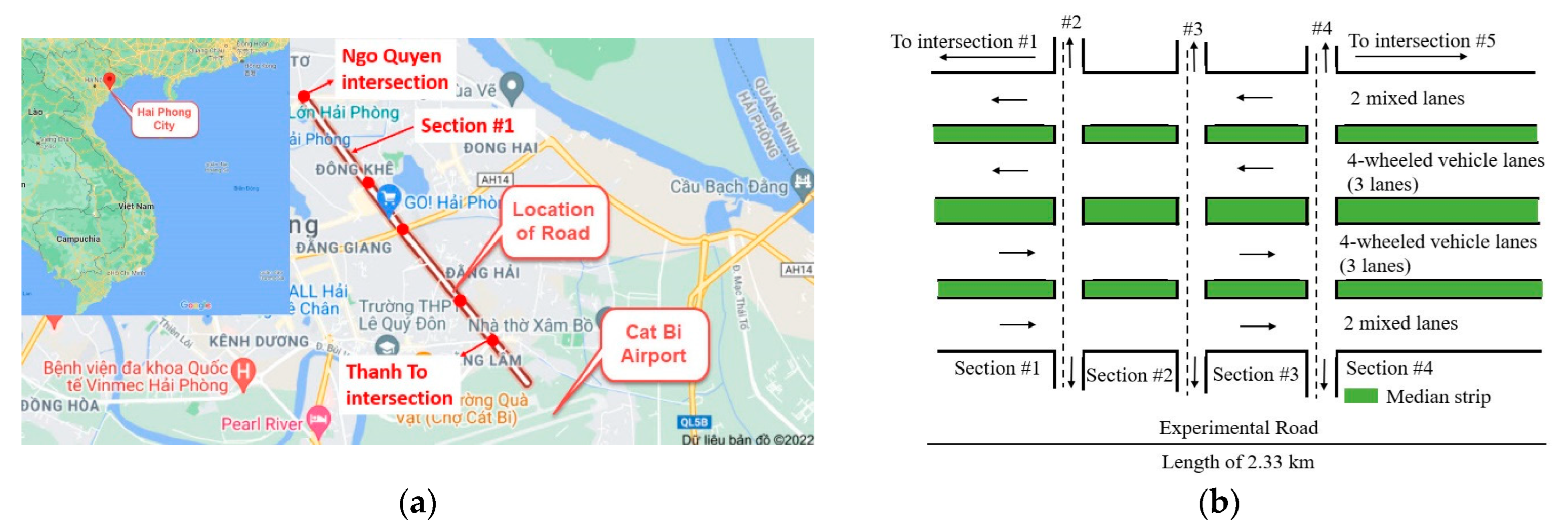
4. Experimental Data Description

4.1. Data Collection

The experimental data are taken from GPS-monitored data of all kinds of vehicles on the Le Hong Phong urban arterial road that is located in Hai Phong city of Vietnam. Hai Phong city is a developing port city among the five most significant cities in Vietnam, with a bustling density of transport. Le Hong Phong urban arterial road is one of the critical routes to connect Cat Bi international airport to the central city. Thus, traffic analysis and forecasting on Le Hong Phong road are essential jobs to improve traffic conditions in the city. However, traffic information acquisition by spot detectors (e.g., loop detectors, cameras) at all the intersections and mid-blocks of that road is complex because most urban streets in Vietnam do not have vehicle spot detectors along the routes as in developed countries. To overcome this difficulty, in this study, we used rich and reliable GPS-monitored data from business vehicles corresponding to Decree No. 86 to predict traffic speed. All GPS-monitored data of business vehicles on the experimental road were collected from 6:00 a.m. to 10:00 p.m. on 1 February to 26 February 2020. The GPS-monitored data updated every 10 s include vehicle coordinates, speeds, driving directions, the uploading time, and vehicle plate.

4.2. Data Pre-Processing

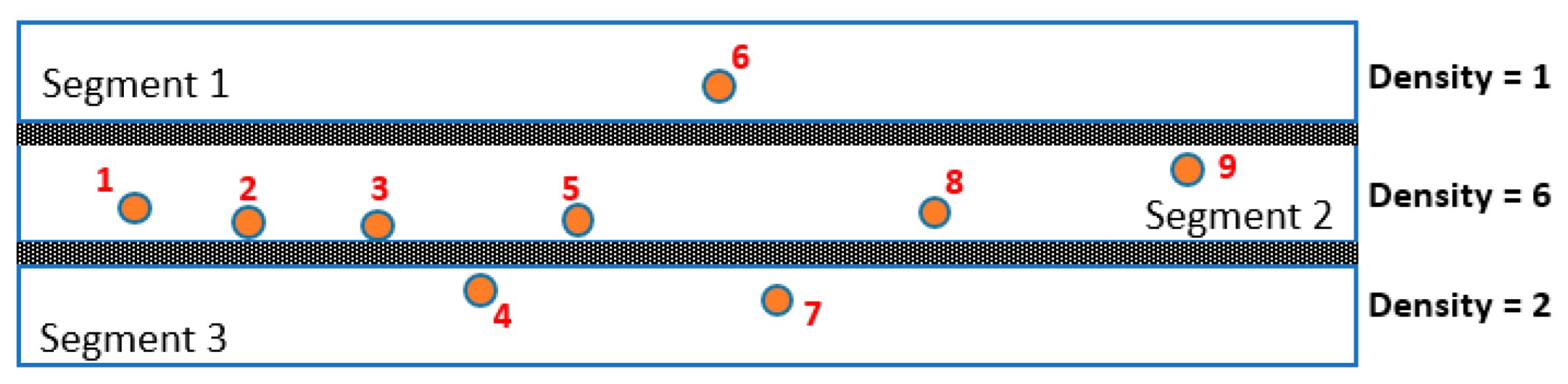
4.2.1. Road Segmentation

The GPS-monitored data acquisition of business vehicles obtained from government agencies encompasses a vast volume every day. It is complicated to compute and analyze traffic flow in the whole road network. Furthermore, this study focuses on TSF. Hence, a part of Le Hong Phong Road and its GPS-monitored data are selected for this study. The experimental road of Le Hong Phong road is a two-way road separated by a median strip that is from Ngo Quyen six-way intersection (Intersection #1) to Thanh to a six-way intersection (Intersection #5) with 2.33 km length and divided into 4 sections (Figure 2a). The cross-section of the experimental road is 64 m, including two central road strips with 10 m widths each for dividing into 3 lanes for cars (4-wheeled vehicles) and two other road strips on two sides with a 7.5 m width each for dividing into two lanes for mixed vehicles, including cars and motorbikes (Figure 2b). Each road section includes four road strips called four segments, and a total of 16 segments is considered in this study.
It can be seen that the survey road section has all of the characteristics of a typical Vietnamese arterial road, including separate lanes for cars, mixed lanes for both cars and motorcycles, and cross-road intersections. The traffic is particularly congested in the early morning and late afternoon, and traffic congestion frequently occurs during peak hours. Based on these characteristics, the experimental investigation on this road section can be expanded to the traffic network in other Vietnamese cities.

4.2.2. Map Matching

Original GPS data are limited to spatial coordinates located on the experimental road. Zone coordinates are extracted from GIS data to create an envelope for the GPS data; then, GPS signals outside this area are discarded. According to the study objectives, it does not consider the period when the vehicles are inactive, so it only uses the recorded data between 6 a.m. to 10 p.m.
To determine each vehicle’s journey in each time frame, the following steps were adopted:
  • Step 1: Filtering points in the time frame under consideration;
  • Step 2: Determining each vehicle’s route (set of points) through the vehicle code;
  • Step 3: Removing the outlines for each route.
Figure 3 shows an illustrated case explaining how to determine a vehicle’s journey. For instance, a vehicle moving on Segment 2 in a time frame that sent 9 signals to the processing center. However, not all of these 9 signals are identified to Segment 2, but two signals were mistakenly received for Segment 3, and the Segment 1 signal was mistaken for Segment 1. To figure out from which road segment the GPS signal from the vehicle comes, the shortest distance is calculated from the GPS coordinates to the route. A vehicle adds its signal density parameter on the road segment in the same 10 min interval to avoid the error that causes the GPS signal of a vehicle to appear on many road segments simultaneously. The road segment with the highest GPS signal density were selected. GPS signals of a vehicle located outside the selected segment were discarded.
It can be seen that Segment 1 has a density of 1, Segment 2 has a density of 6, and Segment 3 has a density of 2. This means that signals 4, 6, and 7 were removed as outliners, and the 6 remaining signals are used to analyze for Segment 2.

4.2.3. Computing Speed

On each segment, the speed is calculated as the average value per time frame. The vehicle’s average speed on the road segment in a particular time frame was calculated as the ratio of the total distance to the whole time traveled by the vehicle according to the GPS signal. The average speed of the entire road segment was determined as the average of all vehicle speeds on that route, as shown in the following equation [54].
v i = 1 1 m j = 1 m 1 v i j
where vi is the i-th segment’s average speed; vij is the speed of the i-th segment’s j-th vehicle; and m is some samples of the i-th segment. The average speed as used to train and predict the traffic speed of the arterial road.

4.2.4. Abnormal Data Processing

The obtained data may have abnormal data, such as missing data due to a problem with the GPS signal transceiver or a traffic problem or no vehicle on the road. Abnormal data can be replaced by the average value for the four adjacent intervals. In case the neighboring intervals are also not informative enough, the data are further supplemented by the average speed data of the same time frame on the road for all days of the month. After the data preprocessing, the obtained data include the following three types of information: (1) time frame (or time interval); (2) average travel speed (in kilometers per hour); and (3) the index of the segment.

5. Experimental Results and Discussion

5.1. Designing LSTM Network and Dataset Preparation

5.1.1. Designing LSTM Network

LSTM network is a major recurrent neural network (RNN) architecture. Many recent types of research have used this network to address the problem of traffic speed forecasting. [35]. This study, based on GPS-monitored data, an LSTM network is used to forecast urban speed. Hochreiter and Schmidhuber first proposed the LSTM network in 1997 [55]. Its primary objectives are to model long-term dependencies and find out the most appropriate time lag for time series problems. The typical LSTM network architecture consists of: an input layer, a recurrent hidden layer, and an output layer. The memory block is the basic unit of the hidden layer in an LMST network. It contains memory cells with self-connections that allow the temporal state to be memorized and a pair of adaptive, multiplicative gating units that manage information flow in the block [35].

5.1.2. Dataset Preparation

We used the sliding window technique to build the learning dataset in ref. [56]. The number of neurons in the LSTM network’s input layer is determined by the size of the sliding window. There is no optimal window size value for all data. This value is determined depending on the characteristics of each data type and can be optimized. After that, we divided the experimental data into three parts, namely a training set, a validation set, and a testing set, which spanned 26 days (1 February to 26 February 2020). The training dataset consisted of the first eighteen days of data. The following four days were utilized to validate the data, while the final four days were used to test it. The proposed model was built using the training and validating datasets. The testing dataset was utilized to make predictions. Before training and testing, the initial data sets were converted to values between −1 and 1 to match the default hyperbolic tangent activation function of the LSTM network.

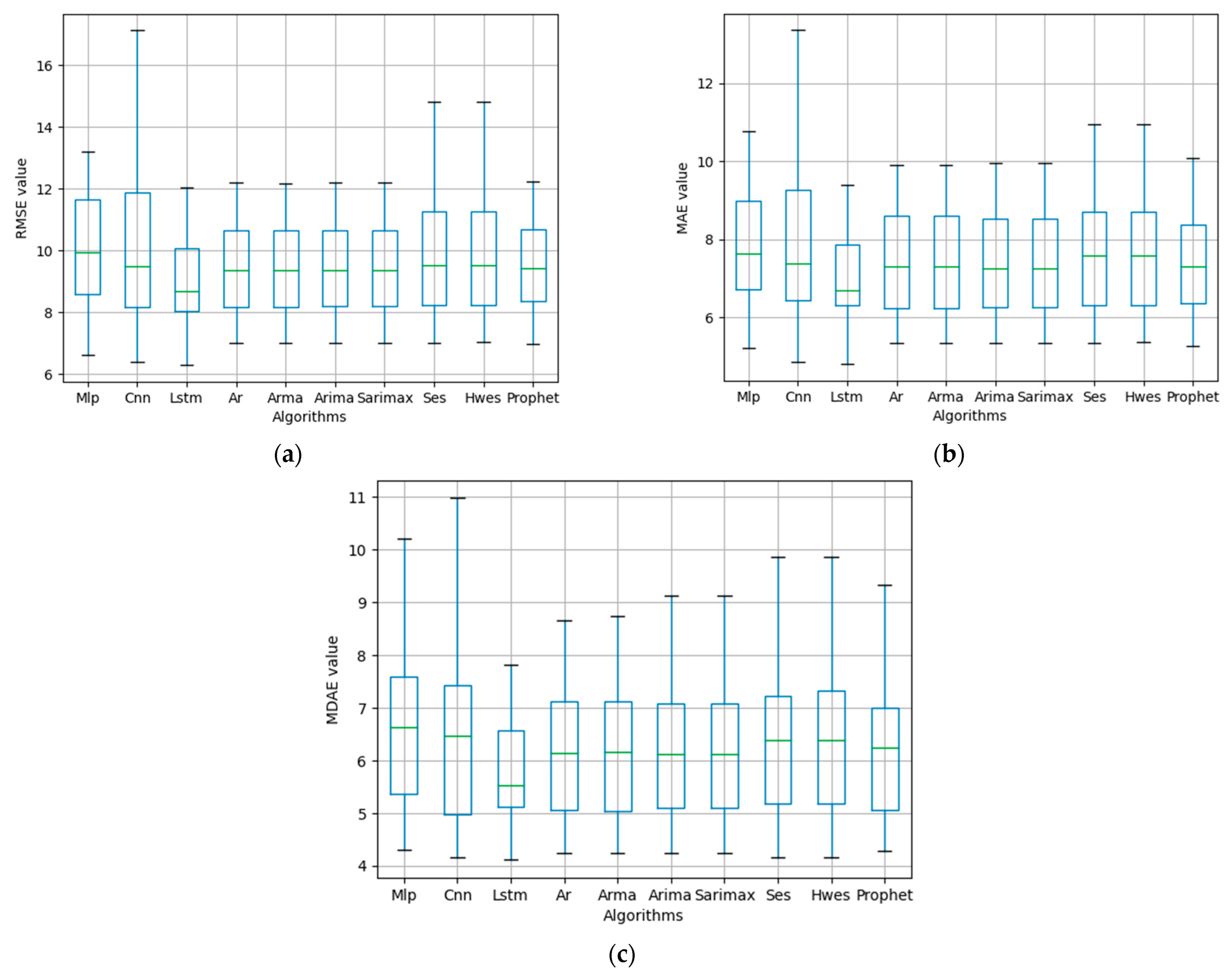
5.1.3. Performance Indicator

Root mean square error (RMSE), mean absolute error (MAE), and median absolute error (MDAE) are used as performance indicators [11,12,57]. They are calculated as follows:
RMSE = 1 n t = 1 n ( ε t ) 2
MAE = 1 n t = 1 n | ε t |
MDAE = m e d i a n | ε t |
where ε t = ( x t x ^ t ) ; n is number of observations; x t is real value; and x ^ t is forecast value.

5.2. Tuning Hyper-Parameters of LSTM Network

Neural networks configurations were exploited experimentally for a given predictive modeling problem. There are three main parameters to be considered: (1) the window size, (2) the number of epochs, and (3) the number of neurons. Firstly, the window size was defined, and then, the number of epochs was identified to find good predictive results for both training and testing datasets, avoiding overfitting. Finally, the number of neurons that influence the network’s learning capacity was adopted. Generally, the more neurons the network has, the better it can learn and comprehend the problem. On the contrary, the training time will increase accordingly. In addition, more learning capacity can lead to a phenomenon called overfitting on the training dataset. To obtain the most accurate assessment, the model was run 10 times for each experimental value, and we took the average result to compare with other experimental values.

5.2.1. Turning the Window Size

The number of neurons in the LSTM network input layer is the first tuning parameter. In this experiment, the model was run with 100 window size values from 1 to 100. Each window size value was run 10 times, and we took the average value. For each segment, the optimal window size value is defined by considering two lines: the blue line corresponds to the RMSE train values, and the orange line corresponds to the RMSE test values. The experimental results show a common point of all 16 segments that the RMSE train curve tends to go down when the window size increases, while the RMSE test tends to increase. The window size value was chosen to satisfy that the RMSE test has the best value. The data for tuning the window size parameter with a segment are shown in Table 2.

5.2.2. Tuning the Number of Epochs

The number of epochs was defined for both RMSE training and RMSE testing parameters. The epoch values were considered in 10 different values from 10 to 100. An epoch value was run 10 times, and we took the average. According to the RMSE value of each different epoch case, the trajectory of each parameter was determined and whether or not it was necessary to determine the epoch values greater than 100. The results show that when the number of epochs increases, the RMSE training decreases, and an upward trend in RMSE testing over the training epochs for all the segments was recognized. Therefore, it can be confirmed that if the epoch value is 10, it is satisfied without the problem of overfitting or underfitting. If the number of epochs is increased, the overfitting phenomenon will be stronger. Thus, it is only necessary to choose an epoch value of 10 to satisfy the desired requirement without considering additional cases of epoch greater than 100.

5.2.3. Tuning the Number of Neurons

This study conducted experiments with neural bands from 5 to 100. When the number of hidden neurons was increased, most of the segments remained the same, and the results did not vary significantly. Only some segments had better results when the number of hidden neurons reached 12; then, the result remained at that level. From this experimental result, we decided to choose the number of neurons as 12 for all segments.

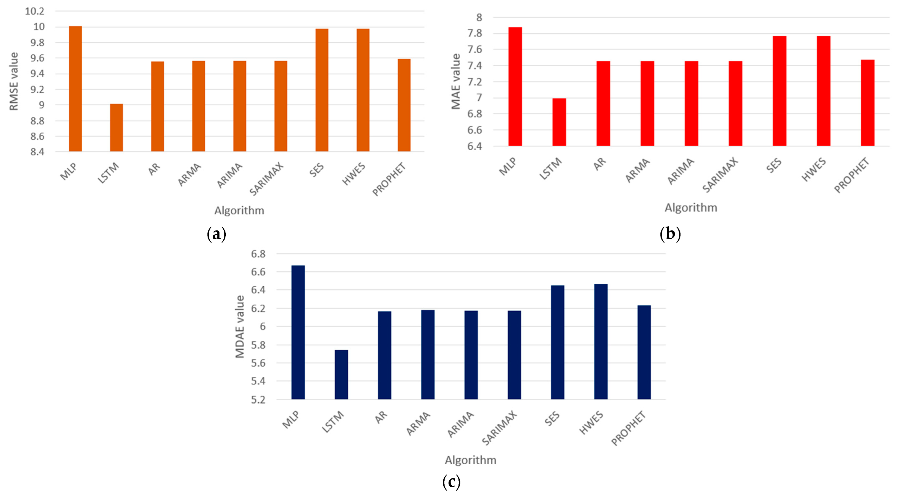
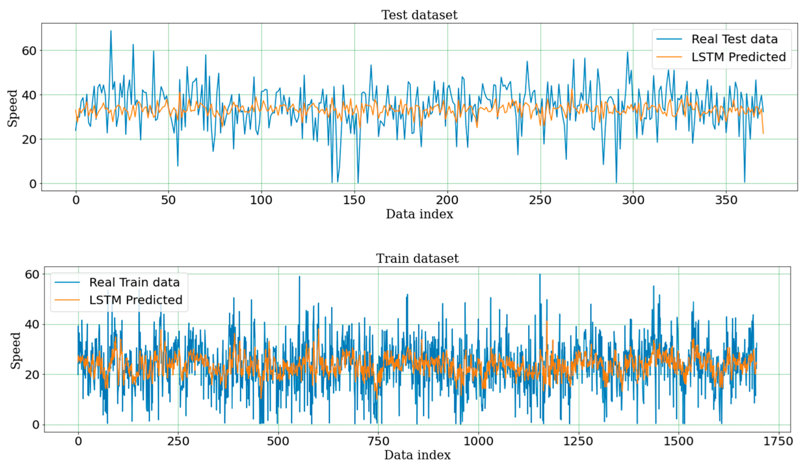
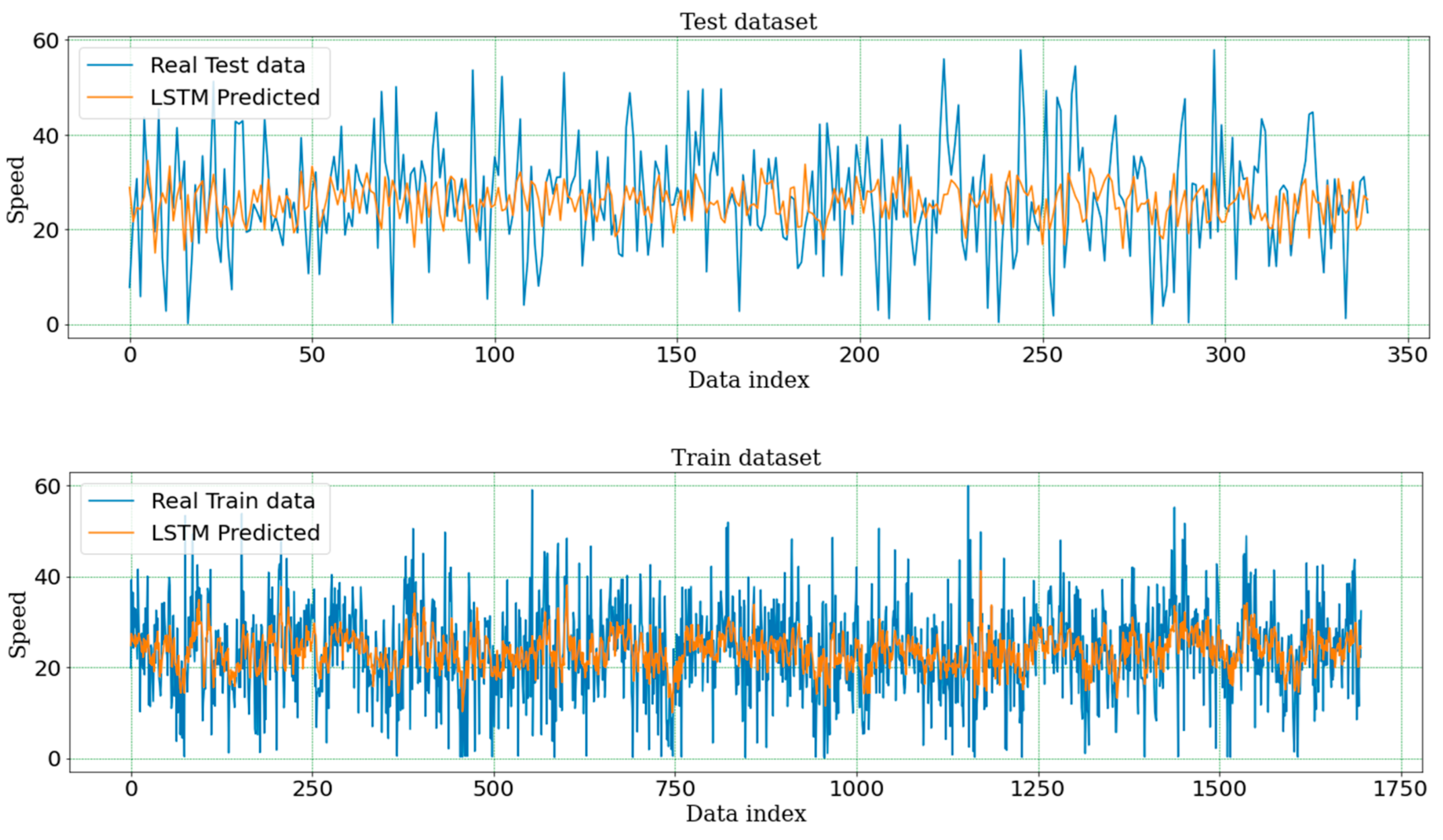
5.3. Forecasting Results and Discussions

After determining the parameters for the LSTM network, we conducted experiments with the speed dataset of 16 segments. To verify the performance of the proposed model, we compared the outcomes with traditional algorithms, including MLP [31,42,50]; the group of algorithms using the autoregressive technique (including AR, ARMA [24], ARIMA, and SARIMAX [25,27,46,58]); the group of algorithms based on exponential smoothing mechanism (including SES and HWES [59]); a state-of-the-art algorithm (i.e., PROPHET [47]); and another deep learning algorithm (i.e., CNN [33,60]). We aggregated the performance indexes for each segment into a single result for all 16 segments. Here, we used box and whisker plots to better represent the statistical data, and we also used additional bar charts to compare the average results of the algorithms. To make it easier to observe, we divided into two comparison groups: first, we compared the LSTM algorithm with a group of conventional algorithms, and the second one was with deep learning algorithms. Figure 4 depicts the performance of the proposed model versus traditional models in a testing dataset.
On all three metrics (i.e., RMSE, MAE, and MDAE), the LSTM network clearly beats traditional techniques. Furthermore, it can be seen that groups of algorithms based on the autoregressive mechanism (i.e., AR, ARMA, ARIMA, and SARIMAX) give quite similar results (approximately 9.56 with RMSE, 7.45 with MAE, and 6.17 with MDAE). These are also the second-best results following the LSTM network. PROPHET’s algorithm gives slightly worse results (with RMSE of 9.59, MAE of 7.47, and MDAE of 6.23). The group of algorithms based on the exponential smoothing mechanism (including SES and HWES) gives much worse results than other algorithms (except the MLP algorithm). These algorithms give an approximate RMSE of 9.97, MAE of 7.77, and MDAE of 6.46. It is pretty surprising that the MLP algorithm gives the worst results when compared to all other algorithms. This result can be explained because the number of iterations we chose in this experiment was still not enough for MLP to achieve the best results (or the phenomenon of under-fitting).
In the above analysis, we compared the results between the algorithms based on the average value of the results over 16 segments. The average value is important, but it does not fully evaluate the performance of an algorithm. Therefore, statistical analysis was performed by plotting the box and whisker figures to represent these parameters. The results corresponding to the three metrics are shown in Figure 5. In these plots, the green line represents the median value. The three values include the 25th and 75th percentiles, and the middle 50% of the data are represented through the box. The mean values give an idea of the average performance of an algorithm, whereas the standard deviation values show the variance. The min and max scores give the range of possible best- and worst-case examples.
From the results on the plots, it can be seen that the LSTM network still gives the best results on all statistical parameters. Specifically, the RMSE of this LSTM network gives a standard deviation of 1.65 and the minimum value of 6.286, while the 25th percentile value is 8.05, the median value is 8.70, the 75th percentile value is 10.062, and finally, the maximum value is 12.048. Meanwhile, the group of algorithms using the autoregressive technique, and the PROPHET algorithm gave similar standard deviation values, with approximately 1.71 and 1.75, respectively. Although it showed a better mean value than MLP, the algorithms based on the ES technique have a larger standard deviation, with approximate values of 2.26 and 2.1, respectively. Figure 5b shows the comparison results based on the MAE metric. This box and whisker chart gives the same results as that of the RMSE metric. The LSTM network still achieves the best results on all statistical parameters, specifically with a standard deviation of 1.327 and a minimum value of 4.80; the 25th percentile value is 6.322, the median value is 6.704, the 75th percentile value is 7.869, and finally, the maximum value is 9.405. Figure 5c shows the similarity of the minimum values of the methods. When using the MDAE metric, the LSTM gives a slightly better minimum value than the other methods. Meanwhile, at the maximum value, LSTM gives much better results than other methods. The MDAE’s value of LSTM is 7.814, while other methods give worse results. The worst one is MLP with a value of 10.201. This plot also shows the difference in the median and mean values of the LSTM algorithm compared to other algorithms similar to the two measurements above. The above results can be seen as follows: Considering all segments, the LSTM algorithm gives the best results on all statistical parameters. This shows that this algorithm not only gives the best prediction results but also gives the results with the lowest stability and volatility. The second best is the group of algorithms using the autoregressive technique. PROPHET is a proven algorithm for accuracy and fast execution. This algorithm has been utilized in several Facebook apps to generate accurate forecasts for scheduling and goal setting. However, when experimenting on the type of these datasets, PROPHET’s algorithm only gave similar results, which were even slightly worse than those using autoregressive techniques. The algorithms using the exponential smoothing technique gave relatively poor results, while its forecasting results were worse than other methods, with low stability and high volatility. The MLP algorithm gave the worst results, which we explained above, due to the phenomenon of under-fitting.
We continued to compare the performance of the LSTM network to that of other deep learning algorithms, such as the CNN algorithm. The results of the comparison are shown in Table 3.
From all three metrics, it can be easily observed that the LSTM algorithm outperforms the CNN. The differences between the two algorithms corresponding to the RMSE, MAE, and MDAE metrics are 1.263%, 14.10%, and 14.72%, respectively. In terms of statistics, it is possible to observe the results on box plots or see detailed information in Table 3. Even though the two minimum outcomes are not significantly different, the maximum values show a big difference between the two algorithms. Considering the RMSE, the LSTM algorithm gives the maximum value of 12.048, while the CNN gives the value of 17.121. Considering the MAE, the values of LSTM and CNN are 9.405 and 13.358, respectively. Finally, for MDAE, the values for LSTM and CNN are 7.814 and 10.976, respectively. Another important statistical information is the standard deviation value. The LSTM algorithm still gives better results than CNN on all three metrics. This shows that the LSTM algorithm gives stable results with small volatility and is much better than the CNN algorithm. The prediction results of the LSTM algorithm with train and test dataset on two sample segments are shown in Figure 6 and Figure 7. The blue line displays the original data, while the orange line represents the forecast data. Observing the sample graphs, it can be seen that, with the training data, the LSTM algorithm gave prediction results that are close to the real data. Meanwhile, the LSTM of testing data gave forecast results that accurately reflected the time-varying laws of real data.
In summary, from the experimental comparison results between the LSTM with other parameters and non-parameters algorithms, it can be confirmed that with the GPS speed data of the experimental road, the LSTM proves to be more suitable than other models. This is proven through not only the average results of all three metrics but also all other statistical parameters, such as standard deviation, min, max, and median.
Through the forecast results along with the forecasting errors of the LSTM, it has also been shown that in our data processing process, from the GPS raw data reading step to the data preprocessing step, filtering abnormal data until the formation of time series data and normalizing data as input for forecasting algorithms have accurately reflected the traffic status of the experimental area, thereby making an important contribution to providing important traffic forecast information for vehicles moving on different time frames.

6. Conclusions and Future Work

In this study, the authors proposed a solution to the problem of speed prediction on urban roads in a city in Vietnam. The proposed model has the main advantage that it is very suitable for parallel multi-lane arterial roads where GPS signal confusion often occurs. The challenges with handling disorders and anomalies with data on these routes have been thoroughly solved. The proposed algorithm allows filtering and identifying those wrong signals, thereby improving the accuracy in determining the average speed of each vehicle and the survey road. The authors have experimented with many prediction methods, including traditional and deep learning networks. The author focuses more on the LSTM by tuning its hyper-parameters to obtain a configuration that fits with traffic speeds using historical GPS data from business vehicles located on a section of 2.33 km on the Le Hong Phong urban arterial road in Haiphong city in Vietnam. The RMSE, MAE, and MDAE were chosen to measure and compare the forecasting performance of the methods. The results have shown that the version of the proposed model using an LSTM network is better than other methods, including MLP, AR, ARMA, ARIMA, SARIMAX, SES, HWES, PROPHET, and CNN. The small parallel multi-lane roads are typical characteristics of Vietnam’s traffic that are not common in many other countries. To the best of the author’s knowledge, there are no studies that deal with a similar problem. Therefore, this study can be regarded as an innovation compared to currently employed methods. However, the drawback of that study is the scope and size of the experimental area. In this study, we selected a testing area with typical traffic patterns found in Vietnamese cities. We hope to see the optimal and suitable solutions for handling the challenges faced by the Vietnamese traffic system.
In subsequent studies, we will focus on improving the model by combining evolutionary computation solutions to automatically optimize deep neural networks hyper-parameters and expanding the scope of the study with a more complicated road network in several Vietnamese cities to achieve more impressive results that can be applied to the entire traffic system in Vietnam.

Author Contributions

Conceptualization, Y.-M.F., T.-V.H., T.L.H.H. and M.-H.C.; Data curation, C.-T.W. and Q.L.; Formal analysis, Q.H.T. and T.-V.H.; Funding acquisition, C.-T.W. and M.-H.C.; Methodology, Q.H.T., C.-T.W., V.T.V. and Q.L.; Project administration, Q.H.T.; Resources, V.T.V.; Software, Q.H.T. and V.T.V.; Supervision, Y.-M.F., T.-Y.C. and T.L.H.H.; Validation, Y.-M.F. and M.-H.C.; Visualization, T.L.H.H. and Q.L.; Writing—original draft, T.-Y.C. and T.-V.H.; Writing—review & editing, T.-Y.C., T.-V.H. and M.-H.C. All authors have read and agreed to the published version of the manuscript.

Funding

This research is funded by the Ministry of Education and Training, Vietnam, under grant number CT.2019.05.02.

Acknowledgments

We thank the Geographic Information System Research Center, Feng Chia University, Taiwan, for editorial assistance in compiling the final version of the manuscript.

Conflicts of Interest

The authors declare no conflict of interest.

References

  1. Wang, X.; Liu, H.; Yu, R.; Deng, B.; Chen, X.; Wu, B. Exploring Operating Speeds on Urban Arterials Using Floating Car Data: Case Study in Shanghai. J. Transp. Eng. 2014, 140, 04014044. [Google Scholar] [CrossRef]
  2. Song, Z.; Guo, Y.; Wu, Y.; Ma, J. Short-term traffic speed prediction under different data collection time intervals using a SARIMA-SDGM hybrid prediction model. PLoS ONE 2019, 14, e0218626. [Google Scholar] [CrossRef] [PubMed]
  3. Liu, Q.; Wang, B.; Zhu, Y. Short-Term Traffic Speed Forecasting Based on Attention Convolutional Neural Network for Arterials. Comput. Aided Civ. Infrastruct. Eng. 2018, 33, 999–1016. [Google Scholar] [CrossRef]
  4. Vlahogianni, E.I.; Karlaftis, M.G.; Golias, J.C. Short-term traffic forecasting: Where we are and where we’re going. Transp. Res. Part C Emerg. Technol. 2014, 43, 3–19. [Google Scholar] [CrossRef]
  5. Lv, Z.; Xu, J.; Zheng, K.; Yin, H.; Zhao, P.; Zhou, X. LC-RNN: A Deep Learning Model for Traffic Speed Prediction. In Proceedings of the Twenty-Seventh International Joint Conference on Artificial Intelligence, Stockholm, Sweden, 13–19 July 2018. [Google Scholar] [CrossRef] [Green Version]
  6. Zhong, S.; Sun, D.J. Analyzing Spatiotemporal Congestion Pattern on Urban Roads Based on Taxi GPS Data. In Logic-Driven Traffic Big Data Analytics; Springer: Singapore, 2022; pp. 97–118. [Google Scholar] [CrossRef]
  7. Lanka, S.; Jena, S.K. Analysis of GPS Based Vehicle Trajectory Data for Road Traffic Congestion Learning. In Advanced Computing, Networking and Informatics-Volume 2; Springer: Cham, Switzerland, 2014; pp. 11–18. [Google Scholar] [CrossRef]
  8. Can, V.X.; Rui-Fang, M.; Van Hung, T.; Thuat, V.T. An analysis of urban traffic incident under mixed traffic conditions based on SUMO: A case study of Hanoi. Int. J. Adv. Res. Eng. Technol. 2020, 11, 573–581. [Google Scholar]
  9. Diependaele, K.; Riguelle, F.; Temmerman, P. Speed Behavior Indicators Based on Floating Car Data: Results of a Pilot Study in Belgium. Transp. Res. Procedia 2016, 14, 2074–2082. [Google Scholar] [CrossRef] [Green Version]
  10. Sari, R.F.; Rochim, A.F.; Tangkudung, E.; Tan, A.; Marciano, T. Location-Based Mobile Application Software Development: Review of Waze and Other Apps. Adv. Sci. Lett. 2017, 23, 2028–2032. [Google Scholar] [CrossRef]
  11. Ye, Q.; Szeto, W.; Wong, S.C. Short-Term Traffic Speed Forecasting Based on Data Recorded at Irregular Intervals. IEEE Trans. Intell. Transp. Syst. 2012, 13, 1727–1737. [Google Scholar] [CrossRef] [Green Version]
  12. Bogaerts, T.; Masegosa, A.D.; Angarita-Zapata, J.S.; Onieva, E.; Hellinckx, P. A graph CNN-LSTM neural network for short and long-term traffic forecasting based on trajectory data. Transp. Res. Part C Emerg. Technol. 2020, 112, 62–77. [Google Scholar] [CrossRef]
  13. Karlaftis, M.G.; Vlahogianni, E.I. Statistical methods versus neural networks in transportation research: Differences, similarities and some insights. Transp. Res. Part C Emerg. Technol. 2011, 19, 387–399. [Google Scholar] [CrossRef]
  14. Xiao, F.; Xue, W.; Shen, Y.; Gao, X. A New Attention-Based LSTM for Image Captioning. Neural Process. Lett. 2022, 54, 1–15. [Google Scholar] [CrossRef]
  15. Malik, S.; Bansal, P.; Sharma, P.; Jain, R.; Vashisht, A. Image Retrieval Using Multilayer Bi-LSTM. In International Conference on Innovative Computing and Communications; Springer: Singapore, 2022. [Google Scholar]
  16. Zhou, J.; Wang, X.; Yang, C.; Xiong, W. A Novel Soft Sensor Modeling Approach Based on Difference-LSTM for Complex Industrial Process. IEEE Trans. Ind. Inform. 2021, 18, 2955–2964. [Google Scholar] [CrossRef]
  17. Peng, L.; Wang, L.; Xia, D.; Gao, Q. Effective energy consumption forecasting using empirical wavelet transform and long short-term memory. Energy 2022, 238, 121756. [Google Scholar] [CrossRef]
  18. Han, S.; Kang, J.; Mao, H.; Hu, Y.; Li, X.; Li, Y.; Xie, D.; Luo, H.; Yao, S.; Wang, Y.; et al. Ese: Efficient speech recognition engine with sparse lstm on fpga. In Proceedings of the 2017 ACM/SIGDA International Symposium on Field-Programmable Gate Arrays, Monterey, CA, USA, 22–24 February 2017. [Google Scholar]
  19. Bhaskar, S.; Thasleema, T.M. LSTM model for visual speech recognition through facial expressions. Multimed. Tools Appl. 2022, 54, 1–18. [Google Scholar] [CrossRef]
  20. Ankita; Rani, S.; Bashir, A.K.; Alhudhaif, A.; Koundal, D.; Gunduz, E.S. An efficient CNN-LSTM model for sentiment detection in #BlackLivesMatter. Expert Syst. Appl. 2022, 193, 116256. [Google Scholar] [CrossRef]
  21. Gu, Z.; Li, Z.; Di, X.; Shi, R. An LSTM-Based Autonomous Driving Model Using a Waymo Open Dataset. Appl. Sci. 2020, 10, 2046. [Google Scholar] [CrossRef] [Green Version]
  22. Kashyap, A.A.; Raviraj, S.; Devarakonda, A.; Nayak K, S.R.; KV, S.; Bhat, S.J. Traffic flow prediction models—A review of deep learning techniques. Cogent Eng. 2022, 9, 2010510. [Google Scholar] [CrossRef]
  23. Liu, D.; Tang, L.; Shen, G.; Han, X. Traffic Speed Prediction: An Attention-Based Method. Sensors 2019, 19, 3836. [Google Scholar] [CrossRef] [Green Version]
  24. Pavlyuk, D. Short-term Traffic Forecasting Using Multivariate Autoregressive Models. Procedia Eng. 2017, 178, 57–66. [Google Scholar] [CrossRef]
  25. Karlaftis, M.G.; Vlahogianni, E. Memory properties and fractional integration in transportation time-series. Transp. Res. Part C Emerg. Technol. 2009, 17, 444–453. [Google Scholar] [CrossRef]
  26. Lam, W.H.K.; Tang, Y.F.; Chan, K.S.; Tam, M.-L. Short-term Hourly Traffic Forecasts using Hong Kong Annual Traffic Census. Transportation 2006, 33, 291–310. [Google Scholar] [CrossRef]
  27. Pan, B.; Demiryurek, U.; Shahabi, C. Utilizing Real-World Transportation Data for Accurate Traffic Prediction. In Proceedings of the 2012 IEEE 12th International Conference on Data Mining, Brussels, Belgium, 10–13 December 2012. [Google Scholar] [CrossRef] [Green Version]
  28. van der Voort, M.; Dougherty, M.; Watson, S. Combining kohonen maps with arima time series models to forecast traffic flow. Transp. Res. Part C Emerg. Technol. 1996, 4, 307–318. [Google Scholar] [CrossRef] [Green Version]
  29. Habtemichael, F.G.; Cetin, M. Short-term traffic flow rate forecasting based on identifying similar traffic patterns. Transp. Res. Part C Emerg. Technol. 2016, 66, 61–78. [Google Scholar] [CrossRef]
  30. Yao, B.; Chen, C.; Cao, Q.; Jin, L.; Zhang, M.; Zhu, H.; Yu, B. Short-Term Traffic Speed Prediction for an Urban Corridor. Comput. Civ. Infrastruct. Eng. 2017, 32, 154–169. [Google Scholar] [CrossRef]
  31. Chan, K.Y.; Dillon, T.S.; Singh, J.; Chang, E. Neural-Network-Based Models for Short-Term Traffic Flow Forecasting Using a Hybrid Exponential Smoothing and Levenberg–Marquardt Algorithm. IEEE Trans. Intell. Transp. Syst. 2011, 13, 644–654. [Google Scholar] [CrossRef]
  32. Chen, H.; Grant-Muller, S. Use of sequential learning for short-term traffic flow forecasting. Transp. Res. Part C Emerg. Technol. 2001, 9, 319–336. [Google Scholar] [CrossRef]
  33. Ma, X.; Dai, Z.; He, Z.; Ma, J.; Wang, Y.; Wang, Y. Learning Traffic as Images: A Deep Convolutional Neural Network for Large-Scale Transportation Network Speed Prediction. Sensors 2017, 17, 818. [Google Scholar] [CrossRef] [Green Version]
  34. Koesdwiady, A.; Soua, R.; Karray, F. Improving Traffic Flow Prediction with Weather Information in Connected Cars: A Deep Learning Approach. IEEE Trans. Veh. Technol. 2016, 65, 9508–9517. [Google Scholar] [CrossRef]
  35. Ma, X.; Tao, Z.; Wang, Y.; Yu, H.; Wang, Y. Long short-term memory neural network for traffic speed prediction using remote microwave sensor data. Transp. Res. Part C Emerg. Technol. 2015, 54, 187–197. [Google Scholar] [CrossRef]
  36. Wang, J.; Chen, R.; He, Z. Traffic speed prediction for urban transportation network: A path based deep learning approach. Transp. Res. Part C Emerg. Technol. 2019, 100, 372–385. [Google Scholar] [CrossRef]
  37. Lv, Y.; Duan, Y.; Kang, W.; Li, Z.; Wang, F.-Y. Traffic Flow Prediction with Big Data: A Deep Learning Approach. IEEE Trans. Intell. Transp. Syst. 2014, 16, 865–873. [Google Scholar] [CrossRef]
  38. Chen, W.; An, J.; Li, R.; Fu, L.; Xie, G.; Alam Bhuiyan, Z.; Li, K. A novel fuzzy deep-learning approach to traffic flow prediction with uncertain spatial–temporal data features. Future Gener. Comput. Syst. 2018, 89, 78–88. [Google Scholar] [CrossRef]
  39. Zhang, W.; Yu, Y.; Qi, Y.; Shu, F.; Wang, Y. Short-term traffic flow prediction based on spatio-temporal analysis and CNN deep learning. Transp. A Transp. Sci. 2019, 15, 1688–1711. [Google Scholar] [CrossRef]
  40. Li, Z.; Xiong, G.; Chen, Y.; Lv, Y.; Hu, B.; Zhu, F.; Wang, F.-Y. A Hybrid Deep Learning Approach with GCN and LSTM for Traffic Flow Prediction. In Proceedings of the 2019 IEEE Intelligent Transportation Systems Conference (ITSC), Auckland, New Zealand, 27–30 October 2019. [Google Scholar] [CrossRef]
  41. Vijayalakshmi, B.; Ramar, K.; Jhanjhi, N.; Verma, S.; Kaliappan, M.; Vijayalakshmi, K.; Vimal, S.; Kavita; Ghosh, U. An attention-based deep learning model for traffic flow prediction using spatiotemporal features towards sustainable smart city. Int. J. Commun. Syst. 2020, 34, 4069. [Google Scholar] [CrossRef]
  42. Lefevre, S.; Sun, C.; Bajcsy, R.; Laugier, C. Comparison of parametric and non-parametric approaches for vehicle speed prediction. In Proceedings of the 2014 American Control Conference, Portland, OR, USA, 4–6 June 2014. [Google Scholar] [CrossRef]
  43. van Hinsbergen, C.; van Lint, J.; van Zuylen, H. Bayesian committee of neural networks to predict travel times with confidence intervals. Transp. Res. Part C Emerg. Technol. 2009, 17, 498–509. [Google Scholar] [CrossRef]
  44. Fusco, G.; Colombaroni, C.; Isaenko, N. Short-term speed predictions exploiting big data on large urban road networks. Transp. Res. Part C Emerg. Technol. 2016, 73, 183–201. [Google Scholar] [CrossRef]
  45. Williams, B.M.; Hoel, L.A. Modeling and forecasting vehicular traffic flow as a seasonal ARIMA process: Theoretical basis and empirical results. J. Transp. Eng. 2003, 129, 664–672. [Google Scholar] [CrossRef] [Green Version]
  46. Williams, B.M. Multivariate Vehicular Traffic Flow Prediction: Evaluation of ARIMAX Modeling. Transp. Res. Rec. 2001, 1776, 194–200. [Google Scholar] [CrossRef]
  47. Taylor, S.J.; Letham, B. Forecasting at scale. Am. Stat. 2018, 72, 37–45. [Google Scholar] [CrossRef]
  48. Haworth, J.; Cheng, T. Non-parametric regression for space–time forecasting under missing data. Comput. Environ. Urban Syst. 2012, 36, 538–550. [Google Scholar] [CrossRef] [Green Version]
  49. Wu, C.-H.; Ho, J.-M.; Lee, D. Travel-Time Prediction with Support Vector Regression. IEEE Trans. Intell. Transp. Syst. 2004, 5, 276–281. [Google Scholar] [CrossRef] [Green Version]
  50. Huang, S.-H. An Application of Neural Network on Traffic Speed Prediction under Adverse Weather Conditions; The University of Wisconsin-Madison: Madison, WI, USA, 2003. [Google Scholar]
  51. Zahid, M.; Chen, Y.; Jamal, A.; Mamadou, C.Z. Freeway Short-Term Travel Speed Prediction Based on Data Collection Time-Horizons: A Fast Forest Quantile Regression Approach. Sustainability 2020, 12, 646. [Google Scholar] [CrossRef] [Green Version]
  52. Yu, R.; Li, Y.; Shahabi, C.; Demiryurek, U.; Liu, Y. Deep learning: A generic approach for extreme condition traffic forecasting. In Proceedings of the 2017 SIAM International Conference on Data Mining (SDM), Houston, TX, USA, 27–29 April 2017. [Google Scholar]
  53. Zhang, J.; Zheng, Y.; Qi, D. Deep spatio-temporal residual networks for citywide crowd flows prediction. In Proceedings of the Thirty-First AAAI Conference on Artificial Intelligence, San Francisco, CA, USA, 4–9 February 2017. [Google Scholar]
  54. Kong, Q.-J.; Zhao, Q.; Wei, C.; Liu, Y. Efficient Traffic State Estimation for Large-Scale Urban Road Networks. IEEE Trans. Intell. Transp. Syst. 2012, 14, 398–407. [Google Scholar] [CrossRef]
  55. Hochreiter, S.; Schmidhuber, J. Long short-term memory. Neural Comput. 1997, 9, 1735–1780. [Google Scholar] [CrossRef]
  56. Yahmed, Y.B.; Bakar, A.A.; Hamdan, A.R.; Ahmed, A.; Abdullah, S.M.S. Adaptive sliding window algorithm for weather data segmentation. J. Theor. Appl. Inf. Technol. 2015, 80, 322. [Google Scholar]
  57. Shcherbakov, M.V.; Brebels, A.; Shcherbakova, N.L.; Tyukov, A.P.; Janovsky, T.A.; Kamaev, V.A.E. A survey of forecast error measures. World Appl. Sci. J. 2013, 24, 171–176. [Google Scholar]
  58. Zhang, H.; Wang, X.; Cao, J.; Tang, M.; Guo, Y. A multivariate short-term traffic flow forecasting method based on wavelet analysis and seasonal time series. Appl. Intell. 2018, 48, 3827–3838. [Google Scholar] [CrossRef]
  59. Billah, B.; King, M.L.; Snyder, R.; Koehler, A.B. Exponential smoothing model selection for forecasting. Int. J. Forecast. 2006, 22, 239–247. [Google Scholar] [CrossRef] [Green Version]
  60. Du, S.; Li, T.; Gong, X.; Horng, S.-J. A Hybrid Method for Traffic Flow Forecasting Using Multimodal Deep Learning. Int. J. Comput. Intell. Syst. 2018, 13, 85. [Google Scholar] [CrossRef] [Green Version]
Figure 1. Workflow of the proposed model.
Sustainability 14 06351 g001
Figure 2. Description of the experimental road. (a) Location of the experimental road. (b) Experimental road with studied sections.
Sustainability 14 06351 g002
Figure 3. Illustrate the case of signal confusion between segments.
Sustainability 14 06351 g003
Figure 4. The performance of the proposed model and traditional models. (a) The testing RMSE; (b) the testing MAE; (c) the testing MDAE.
Sustainability 14 06351 g004
Figure 5. Box and whisker plot of testing performance indicators. (a) Summarizing RMSE testing; (b) summarizing MAE testing; and (c) summarizing MDAE testing.
Sustainability 14 06351 g005
Figure 6. Prediction results of LSTM with training and testing datasets on Segment 1.
Sustainability 14 06351 g006
Figure 7. Prediction results of LSTM with training and testing datasets on Segment 2.
Sustainability 14 06351 g007
Table 1. A comparison table of TSF models.
PaperModelsExperimental DataExperimental AreaIntervalSource
Parametric Approaches
Pavlyuk et al. [24]ARIMA, VARMAFrom 29 May 2016–3 September 2016 (13 weeks)Minnesota, USA. Considers only one direction (from southeast to northwest)5 minLoop detector
Pan et al. [25]ARIMA, ES, MLPFrom 1 November 2011–7 December 2011Entire LA county highways and arterial streets5 minLoop detector
Voort et al. [26]Kohonen-ARIMAJuly and August 1990Beaune, where the flow along three feeder motorways converges onto a single motorway30 minLoop detector
Fusco et al. [27]Seasonal ARIMAGPS of private vehicles from August to December 2014The primary urban road network of the EUR district in the southern area of Rome5 min100,000 GPS-equipped private vehicles
Williams et al. [28]ARIMAXFrom months of July and August from 1984 to 1990.Four French motorway sites30 minLoop detector
Non-Parametric Approaches
Filmon et al. [29]Enhanced K-NNMultiple datasets were collected from 3 months to 12 months.Different regions in the United States and United Kingdom15 min
Baozhen Yao et al. [30]SVMOne month of taxi dataFoshan30 sGPS taxi data
Kit Yan Chan et al. [31] Hybrid exponential smoothing method and the Levenberg–Marquardt (LM) algorithm12 traffic flow data sets (from weeks 38, 41, and 52 in 2008 and weeks 2, 12, and 27 in 2009)Reid Highway and Mitchell Freeway intersection, western Australia1 min
(the 2 h peak traffic period (7:30–9:30 a.m.))
Two detector stations
Muhammad Zahid et al. [32]Fast forest quantile regression (FFQR)From around 06:00 a.m. to 12:00 p.m.A portion of Beijing’s 2nd freeway Ring RoadDifferent time intervals, including 5, 10, 15 minLoop detector
Deep Learning Approaches
Ma et al. [33]Deep convolutional neural networks (deep CNN)From 1 May 2015 to 6 June 2015 (37 days)Two sub-transportation networks of Beijing.2 minTaxicab GPS
Arief Koesdwiady et al. [34]Deep belief networks (DBNs)Mixed between history weather and traffic data from 1 August 2013 to 25 November 2013.San Francisco Bay Area of California, 47 freeways.30 s (then aggregated into 5 and 15 min.The inductive-loop sensors
Xiaolei Ma et al. [35]Long short-term neural network (LSTM NN),From 1 June 2013 to 30 June 2013 Two separated locations in a major ring road around Beijing2 minTraffic microwave detectors in Beijing
Jiawei Wang et al. [36]CNN-LSTM, bi-directional LSTMThree months, from 23 January 2018 to 22 April 2018Xuancheng, China. A road network consists of 112 road segments5 minAutomatic vehicle identification (AVI) detectors
Yisheng Lv et al. [37]Stacked autoencoderThe first three months of the year 2013Freeway systems across California.30 s (aggregated to 5 min)15,000 loop detectors
Chen et al. [38]Combination of the fuzzy method and the deep residual convolution networkThe taxicab GPS dataBeijing, China48 samples per dayTaxicab GPS
Zhang et al. [39]A combination model of spatial-temporal analysis and CNN algorithmFrom all weekdays from 1 January to 31 March 2016I-5 Freeway in Seattle, USA5 minLoop detector
Li et al. [40]A graph and attention-based LSTM networkFrom 1 April 2016 to 31 August 2016Caltrans performance measurement system (PeMS) database5 min100 detector stations
Vijayalakshmi et al. [41]Attention-based CNN-LSTMBetween 1 August 2018 and 30 October 2018The location Interstate 405-Northbound5 minDetectors at 37 locations
Table 2. Tuning the window size parameter with a segment.
NoSegment NameOptimal Window
Size Value
NoSegment NameOptimal Window
Size Value
1Segment 1119Segment 996
2Segment 24210Segment 1035
3Segment 37311Segment 1165
4Segment 49712Segment 1216
5Segment 54613Segment 1394
6Segment 64714Segment 1411
7Segment 74015Segment 1556
8Segment 84716Segment 1697
Table 3. Statistical parameters comparison between LSTM and CNN.
MetricModelCountMeanStd.Min25%Median75%Max
RMSE TestCNN1610.3763.2336.4058.1599.50211.86717.121
LSTM169.0121.6526.2868.0528.710.06212.048
MAE TestCNN168.1422.654.8696.4367.3939.25813.358
LSTM166.9941.3274.8026.3226.7047.8699.405
MDAE TestCNN166.7362.2654.1594.9816.4617.43410.976
LSTM165.7451.1724.1145.125.5236.5647.814
Publisher’s Note: MDPI stays neutral with regard to jurisdictional claims in published maps and institutional affiliations.

