
Economic Sustainability and ‘Missing Middle Housing’: Associations between Housing Stock Diversity and Unemployment in Mid-Size U.S. Cities


Department of Geography and Sustainable Planning, Grand Valley State University, Allendale, MI 49401, USA
Sustainability 2022, 14(11), 6817; https://0-doi-org.brum.beds.ac.uk/10.3390/su14116817
Submission received: 2 February 2022
/
Revised: 30 May 2022
/
Accepted: 31 May 2022
/
Published: 2 June 2022
(This article belongs to the Special Issue Economic Development and Inequality: The Role of Cities and Regions)
Abstract
:Single-family detached homes—the lowest-density housing type—continue to dominate the U.S. home construction industry. These homes are carbon-intensive and automobile dependent; the built environments they produce militate against civic relations and attitudes. Cities need to increase density, support multimodality, and develop social capital, but these issues are not propelling cities to diversify their housing stock. The objective of this research is to facilitate this shift by establishing economic arguments for increased density and housing diversity. Municipal-level U.S. Census data is used to explore the interurban relationships between diversity in housing stocks and unemployment rates in 146 mid-size American cities. A measure of diversity, Shannon’s H, is applied to housing stock and found to be strongly associated with lower unemployment for workers over 25 years old after controlling for measures of urban social burden. In contrast to the much-heralded “trade-offs” between environmental quality, social equity, and economic development, these findings suggest that the dense, walkable, low-carbon city, and the economically sustainable city might be the same place.
1. Introduction
Cities are hard pressed to build more affordable housing. However, expensive single-family detached homes (SFDH) continue to dominate the U.S. home construction industry. Despite large state and regional variations, two-thirds of all units produced in the U.S. between March 2019 and 2020 were SFDHs (HUD, 2020). The SFDH approach to housing produces built environments that are carbon-intensive [1,2], automobile dependent [3], and which militate against civic relations and attitudes [4,5,6,7]. With climate change and other threats to societal sustainability looming, U.S. cities need to quickly shift towards a housing paradigm that reduces housing costs, increases density, supports multimodality, and helps develop social capital.
Large, multifamily buildings (LMFBs) can improve outcomes in the areas mentioned above, particularly in per capita carbon emissions [8,9]. Of the nearly 500,000 multifamily units produced in the past year, 92% were in buildings with 5 or more units [10]. However, LMFBs can have sustainability-related problems of their own, including poor air quality, reduced social connectivity, and other issues [11,12,13]. Leaving those issues aside for the purposes of this discussion, we can acknowledge that LMFBs alone do not adequately compensate for the shortcomings of the SFDH housing paradigm.
The answer for some in the planning community is to increase the supply of middle-range buildings containing 2–10 units [14]. This “missing middle housing” is among the most sustainable of all built environments across myriad indicators, including walkability and socio-political measures [15,16,17]. For example, the sort of neighborhood interactions and group participation that support social sustainability occur most at medium densities [18]. While the construction of LMFBs is a welcome addition to carbon-intensive U.S. built environments, it cannot be said that a city is truly diversifying its housing stock without also increasing the number of missing middle-type structures.
Increasing the share of missing middle housing is necessary in the era of climate change and social sustainability [14]. However, local planning departments have not succeeded in shifting housing construction towards either higher density or increased diversity by arguing that more sustainable built environments have better public health, environmental quality, or quality-of-life outcomes. On the contrary, density has been erroneously associated with every sort of urban ill, while the benefits of density have been mostly ignored [19]. Furthermore, numerous regulatory barriers towards constructing missing middle housing exist in almost every U.S. city: zoning ordinances tend to favor SFDHs and automobile dependency (e.g., Grand Rapids Zoning Ordinance, Section 5.1.03), with some notable exceptions, such as Minneapolis’ recent banning of single-family zoning. While these regulations exist ostensibly to “…promote the public health, safety, and general welfare…” (e.g., Michigan Zoning Enabling Act, Section 125.3201), perhaps ironically, the well-established arguments of environmental and social sustainability have proven to be largely inadequate for sparking local change in U.S. built environments, much less for prompting a nation-wide shift towards regulations that favor the construction of missing middle housing.
What may be lacking is research showing that sustainable built environments, such as those with adequate missing middle housing, have better economic outcomes. Despite both urban and sustainable development policy being dominated by economic issues such as job growth, wages, and employment [20,21,22,23], economic research on housing diversity is lacking. After a lengthy search of the literature, researchers found no extant research on the association between unemployment and housing diversity. One reason for this lack of published evidence may be that nobody is looking for it. Instead of seeking out associations between economic sustainability and sustainable urban development, the dominant paradigm in sustainable urban planning suggests that economic, social, and environmental sustainability are all in conflict. For example, Campbell (1996) asserts that there are necessary “trade-offs” between economic development and sustainable land use, represented in the “Planner’s Triangle” [24]. “The planner must reconcile not two, but at least three conflicting interests: to grow the economy, distribute this growth fairly, and in the process not degrade the ecosystem” (ibid. p. 297; emphasis added). Campbell argues that conflicts between environmental, economic, and social goals create inherent contradictions in sustainable development.
Moreover, this Venn diagram-based view conceptualizes the economy as something distinct from and independent of the environment and civil society. However, others argue that this view produces the very conflicts about which Campbell writes [25]. In contrast to conflict, complementarity may be what actually characterizes the links between the three spheres. Others have asked, “What if the economically sound, socially just, and environmentally healthy city is all the same place?” [26].
To arm planners with empirical research that can help shift U.S. cities towards regulatory schemes that support the low-carbon environments that missing middle housing provides—as well as shed light on the question of “trade-offs versus complementarity” in sustainable urban development theory—this study uses cross-sectional data to answer the following question: “Is there a relationship between local unemployment and diversity of housing stock in U.S. municipalities?”
2. Materials and Methods
Aggregate worker characteristics, local firms and industry type, demographics, costs of living, education levels, and more are each important factors for determining urban economic outcomes. However, the built environment itself is also of critical influence [27,28]. Unfortunately, isolating exactly what about the built environment matters and the limit of its effect is both understudied and undertheorized.
2.1. Measures of the Built Environment
Parsimonious measures of the built environment are scarce. Since population density is such an obvious and fundamental property of the built environment—as well as its critical relationship to carbon emissions—it remains the urban research workhorse. Despite being parsimonious, density is increasingly being shown as an overrated proxy of the built environment with many shortcomings [29]. For example, densely populated cities can still be highly automobile dependent [30]. Many outcomes that have been attributed to density are in fact density’s correlation with multimodality [31]. Though it is necessary to control for density in urban, economic, and built environment research, it is far from sufficient.
Direct measures of the built environment often focus on other conceptions of density, such as block density and street patterns [32,33,34]. Although parsimonious, block density is a measure of relationships between physical space: it does not reflect which places are being related, i.e., housing types and land uses. Again, diversity in the built environment is only implied. Dense street patterns are neither necessary nor sufficient conditions for housing diversity: they can contain only SFDHs, only LMFBs, or no housing at all.
Land use mix is a useful construct, there being several ways to operationalize it [35]. However, a mix of land uses does not necessarily equate to diversity in housing: the notion of “mixed-uses” is often satisfied by a mix of commercial and residential high-rises, or by the proximity between commercial areas and monotonous housing districts. Indices of sprawl and compaction can include land uses and block density, but they lack parsimoniousness, and have other considerable short-comings [36,37,38].
Measures of multimodality are increasingly being shown as useful, and even critical variables in social science research [39]. Multimodality can be defined as the capacity of a city to provide non-SOV travel and commuting. Since this capacity is largely (but not entirely) determined by the built environment, diversity in commuting modes is a useful proxy for the built environment. One measure, commute mode diversity (CMD), is the percentage commuters travelling by means other than an SOV. Several key economic outcomes and indicators are associated with CMD. For example, in mid-size U.S. cities, CMD is associated with less overspending on housing costs, increased home property values, as well as less income inequality between whites and African Americans and between men and women [40]. Multimodal travel is supported by higher population densities, and density is associated with housing diversity. Nevertheless, CMD is an inadequate proxy for housing diversity: both monotonous high-rises and densely packed SFDHs can support non-SOV travel.
In summary, the urban social sciences lack robust, parsimonious, and direct measures of diversity in the built environment. However, since CMD is a proxy for diversity in travel, it provides a useful point of departure for considering diversity in housing.
2.2. Measuring Diversity, Not Dominance
Commute mode diversity (CMD) is the percentage of workers who use modes other than SOV for commuting. As such, it is merely a measure of dominance: it captures every mode a non-SOV commuter might use. This lumping together of modes can be justified because diversity is inherent to the measure: most non-SOV commuters use more than one mode on a typical day; even a walk to the bus stop is by definition multimodal. Furthermore, different travel modes are complementary, and not necessarily competitive with each other: built environments that produce walkability often also produce bike-ability and support transit use, whereas automobile-centered built environments present substantial barriers to every other travel mode. There are good reasons to study the individual impacts and drivers of mode choice, such as determining which modes best support a reduced dependency on cars. Still, it is not critically important to distinguish between the different modes when analyzing the interurban impacts of multimodality.
CMD’s corresponding variable in housing diversity is simply lumping all types of non-SFDHs together into one percentage of the total. The obverse, the percentage of housing that are SFDHs, is used in urban research, especially as a variable in mode choice research [41]. Bramley and Power (2009) use the percentage of detached housing to proxy housing diversity’s relationship to several social indicators [42]. They found inconclusive results, writing that
“More dense, compact urban forms, and their associated housing types, tend to be associated with somewhat worse outcomes in relation to dissatisfaction with the neighbourhood and perhaps more strongly with the incidence of neighbourhood problems. At the same time, it is clear that the sociodemographic composition of neighbourhoods, particularly in terms of concentrations of poverty and social renting, has a larger impact on these outcomes than urban form.” (p. 46).
Unlike CMD’s use of dominance as a proxy for diversity in transportation, lumping together non-dominant types of housing is not a useful approach for assessing the interurban impacts of diversity in housing. First, it is hard to imagine types of housing working together in a complementary way for the benefit of an individual resident in the same way that different non-SOV travel modes complement each other to facilitate the individual traveler’s commute. One might use multiple modes of travel each day, but few people use multiple modes of housing, even over the course of several years. Additionally, it is likely that demand for SFDHs is less elastic to the presence of new multifamily units than SOV commuting is elastic to increased multimodality [43,44]. Thus, the percentage of non-SFDHs might be a useful variable, but it is not an adequate measure of housing diversity.
Shannon’s H
Diversity can be “…quantified for any dataset where units of observation have been classified into types” [45]. The construct of diversity can be operationalized in numerous ways. The basic measure is a simple count of the different types of cases which exist within a community: the number of types (e.g., species) in each system indicates the systems’ comparative richness [46]. Richer communities containing more types are considered more diverse. More advanced measures are those which also consider each type’s proportion of the total number of cases, or evenness [47]. Since we know that SFDHs and LMFBs dominate housing, it is more appropriate for the present study to focus on the impact of evenness. Though there are numerous ways to capture evenness, Shannon’s H is used here since it is sensitive to the presence of rare types. Shannon’s H is calculated as: H’ = −pi∑lnpi where pi is the proportion of objects found in category i. This proportion is estimated as pi = ni/N, where ni is the number of objects in category i, and N is the total number of objects in the system. Since the pis will be between zero and one, the natural log makes the terms of the summation negative: we take the inverse of the sum. The index increases if either the number of categories or the evenness of the proportion in the categories increase. This corresponds well to the “missing middle” in housing: cities are likely to exhibit fewer of these types, and we are interested in their importance. One advantage in using Shannon’s Housing H (SHH) is that we have a fixed number of categories (viz. housing types). One caveat is that Shannon’s H is sensitive to sample size; future research can determine the most suitable measure.
2.3. Conceptual Framework
Why would diversity in housing have a relationship to employment? On average, more diversity in housing provides greater housing options to a wider proportion of the city’s total potential workforce. Every city has some diversity in jobs, and thus, some diversity in workers, with a wide range of incomes, tastes, and expectations. There are at least three principles from the field of economics which we can use to conceptualize the relationship between housing diversity and employment: diminishing returns, redundancy, and modularity.
Economists explain how increasing the number of identical workers beyond the number needed to complete a task leads to a diminishing marginal product of labor: more workers doing the same work diminishes the value of the marginal worker. Regarding diminishing returns, Page (2010) writes that the central limit theorem, the diversity central limit theorem, and the factor limit theorem “… all imply that diversification reduces performance variation …” [48] (p. 118). Page asserts that “… in most cases, the effect of adding more members of a species to an ecosystem will also satisfy diminishing returns to productivity” (p. 184).
The same holds true for increasing the proportion of the dominant housing type in a city. If a central city only builds costly SFDHs, then the marginal SFDH unit may bring diminishing returns, resulting in unoccupied SFDH units. This approach also increases competition for missing middle housing in the central city, increasing their rental costs: workers who manage to find an appropriate unit will simply overpay on housing. This leads to the question of the appropriate mix of housing to match market demand, but that is a different question than the impact of diversity in housing on unemployment.
Redundancy is the availability of types that substitute for another. Too much redundancy can be a problem in some systems by reducing diversity (i.e., if everything is a substitute, then there is less actual diversity) (ibid. pp. 227–230). Extreme cases aside, greater diversity in species supports system function through increased redundancy: “… if a system contains redundant parts, then it will be more robust to the failure of one of the parts.” (ibid. p. 227). In the example above, the marginal SFDH fails to satisfy a worker who desires a duplex. However, many workers may consider a fourplex an adequate substitute for a duplex, and vice-versa. In contrast, it is less likely that workers consider non-SFDHs to be adequate substitute for a SFDH. Thus, a larger number of species can lead to an increase in redundancy.
Modularity in the spatial context of built environments implies that cities with one type of housing cannot easily adapt to changing values and conditions. One such changing condition is in Millennials and Gen Zs shifting towards urban living [49]. The city with greater housing diversity has a greater capacity for adaptation over time, whereas the monotonous city lacks “spatial modularity” [50] (p. 104). Like redundancy, too much modularity can create problems. However, U.S. cities as a whole tend toward the other side of the problem spectrum: too little modularity.
While the conceptual framework above suggests a relationship between housing diversity and employment, empirically locating the association between them faces serious methodological challenges.
2.4. Confounding Factors in Housing Diversity and Employment
Attempts to identify relationships between aspects of the urban built environment and socio-economic outcomes are often confounded by myriad factors (see, for example, Bramley and Power, 2009) [42]. Chiefly, there are intervening conditions (viz. distinct social burdens carried by central cities) to which unemployment is positively correlated, such as market and policy failures. For example, if central cities have more diverse housing than suburbs, and endure greater social burdens than suburbs, then there will be a positive correlation between housing diversity and social problems. This correlation will bias associations between housing diversity and employment. Thus, there is a need to control for the outcomes of market and policy failures that correlate with housing diversity.
Which variables capture the economic conditions that are associated with both unemployment and housing diversity such that we can isolate the relationship, if any, between employment and housing diversity? Unemployment itself is often used to indicate a troubled city; unfortunately, that is the dependent variable in this work. However, the population-employment ratio is a useful measure of an economy’s ability to create jobs [51,52].
Higher median household incomes have long been associated with lower unemployment levels. Yet, the relationships are complex. For example, median household incomes can rise when the economy is poor because workers increasingly share household space [53]. Regional cost of living indices are also problematic control variables in interurban research [54,55]. Statistical models need to control for the urban social burdens that market and policy failures produce which obscure the relationship between housing diversity and employment.
Measures of Urban Social Burden
Home ownership rates play a role in regional economic outcomes, and have been associated with unemployment [56,57,58,59]. It would be a mistake to assume that high rental cities are necessarily burdened: well-to-do resort towns often have a high proportion of rentals. However, in 146 randomly distributed cases across the United States, the percentage of rental housing should capture the effect of municipal property markets where wealth is extracted from property and, on average, deposited in other communities.
Housing vacancies can be the simple result of construction outpacing demand. But ongoing lack of demand (from all its sources, e.g., crime, unemployment, etc.) can lead to burdened cities when municipal tax receipts fall. Rentiers who are not receiving rents are also not reinvesting that money into the community, to the extent that they live in the community. On average, burdened cities should have a higher percentage of vacant residential property.
Workers’ needs for state economic assistance does not necessarily mean a city is burdened: spikes in assistance can be temporary. Moreover, both employed and under-employed people often receive food assistance. Overall, however, the percentage of the population receiving food stamps should indicate market and policy failures in municipal economies.
Variables such as the percentage of residents overspending on housing and ‘tenure gap’ (e.g., the difference in overspending between renters and owners) are important measures of inequality. They are also problematic. For one, the overspending threshold of 30% of resident income is arbitrary, and it focuses on burdened demographics versus the city as a whole. Tenure gap is a useful measure of inequality, but low-performing municipal economies can be considered equitable along this measure. In contrast, median rent as a percentage of income is more continuous, and, being based on the median, better reflects general market and policy failures that burden municipalities.
The population-employment ratio is defined by the Bureau of Labor Statistics as, “the ratio of total civilian employment to the civilian noninstitutional population”. Since it accounts for the impact of labor force participation and unemployment, “…it is a useful summary measure when those forces place countervailing pressures on employment” [51]. Here it is used as a robust measure of an economy’s ability to provide jobs for its workers.
2.5. Level of Analysis
Part of the gap in research on the built environment and economic outcomes such as unemployment can be attributed to the focus on the regional level of analysis. Cities are rightly thought of as regional phenomena: labor and housing markets often stretch far beyond core city boundaries. Also, regions tend to rise and fall together, suburbs and central cities alike [60,61].
However, regional governance is not supported by the U.S. Constitution, and is therefore largely absent or, when present, toothless. Plus, while the economic fortunes of suburbs and core cities may be closely tied, their built environments tend to be very different, with walkable centers and automobile dependent suburbs. Looking at larger aggregated regional measures such as metropolitan statistical areas and commuter zones obfuscates the distinction between these different built environments. Cities can also be studied at the level of the core municipality. The main advantage is that central cities have less variability in their built environments than do larger geographies. Furthermore, the municipal level of geography speaks directly to the level of governance at which most planners and policy makers operate. However, social and economic outcomes in central cities are heavily impacted by neighboring jurisdictions, especially large, adjacent cities.
2.6. Case Selection
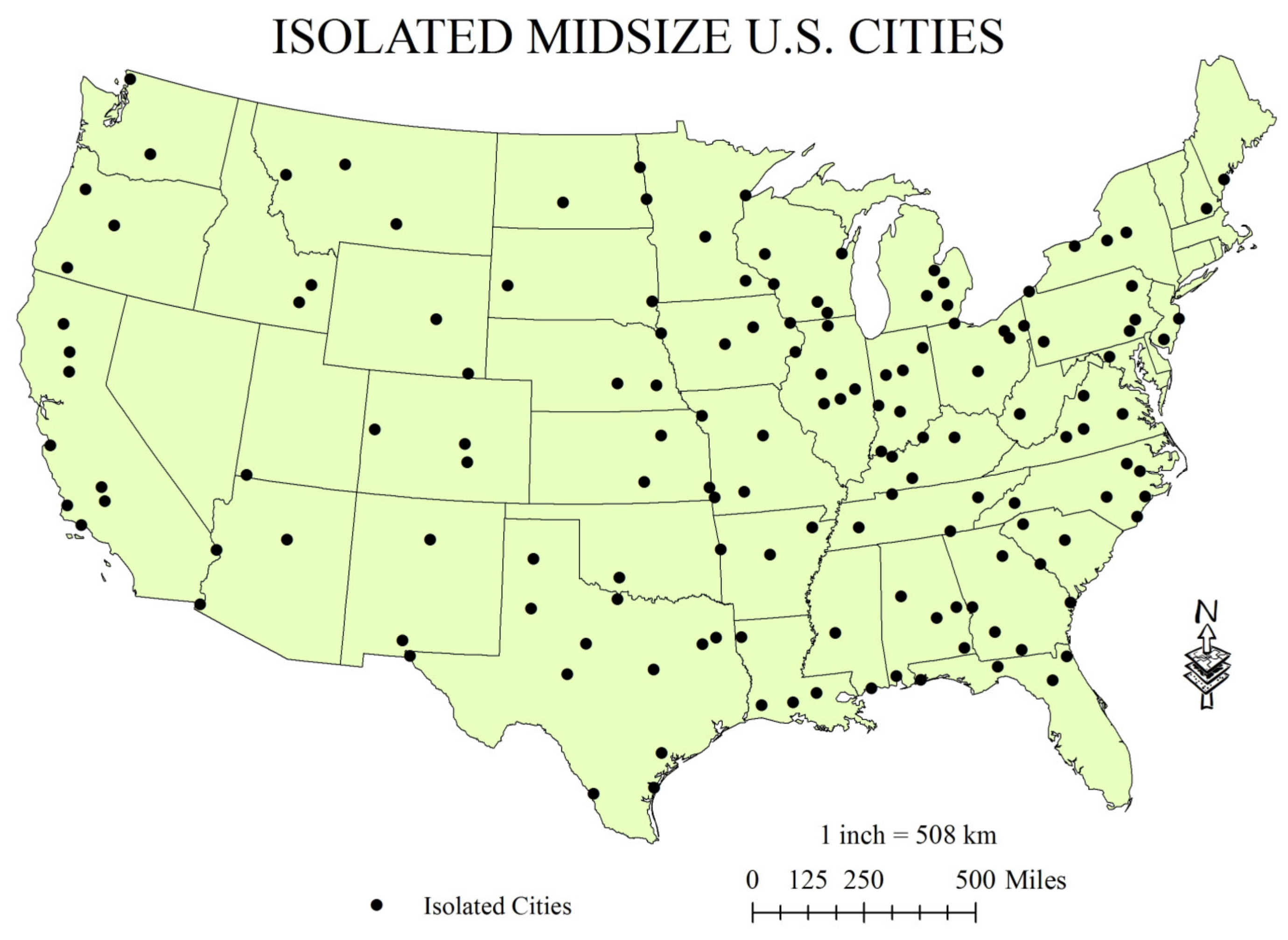
The method of urban scholars Harvey Molotch and Richard Appelbaum employs a pair of decision rules to identify cases which limit the impact of adjacent jurisdictions (e.g., Appelbaum, 1978) [62]. The universe of cities is reduced to all ‘places’ identified by the U.S. Census as having a population of at least 50,000. In 2013, they numbered 792. The second decision rule limits cases to those places being no less than 20 miles border to border from the nearest city of 50,000 or more. As 26 min is the average total commute time in the United States, this 20-mile distance border to border captures the bulk of commuting. A third decision rule is added to this case selection: having an elected, policy-making government. This rule excludes most of the relatively less-governed ‘Census-designated places’ from the set. The three rules yield 146 cases which are randomly distributed (Moran’s I = 0.048, z = 1.62, p < 0.011) across the United States (see Figure 1).
This unit of analysis—the semi-isolated, mid-size city—has unique advantages over other available units, including less overlap between distinct labor and housing markets. This approach also reduces the need to control for spatial lag effects, such as the ‘spillover effects’ from the policies of nearby cities. Empirically, interurban analyses are improved when using a population of cases. These 146 municipalities are not merely a ‘sample’; they constitute all such places in the United States. In short, the unit of analysis is the relatively isolated U.S. city with a population over 50,000.
2.7. Dependent Variable: Unemployment
The overall unemployment rate of a city is important to know. However, the relationship between housing and employment requires finer granularity by age groups, because this relationship is confounded by young people who largely do not choose a home in order to access labor markets, whereas adults often do. Furthermore, the mean retirement age is uneven from city to city, and elderly people also endure unique housing burdens. Unemployment data comes from the U.S. Census table S2301 measured at the level of place, ages 16 and over. The data is further subdivided into five categories: workers aged 16–19, 20–24, 25–44, 45–54, and 55–64. The measure itself is the number of unemployed persons divided by the number of people in the workforce (i.e., those working or looking for work), multiplied by 100. Unlike the employment-population ratio, this figure does not include people who are not looking for work.
2.8. Basic Statistical Model
The first model’s six variables represent elementary urban characteristics, and include standard choices such as population, median household income, and percentage of population with bachelor’s degrees, plus Shannon’s Housing H (SHH). All values are derived from 2013 U.S. Census 3-year estimates at the level of place (files DP05, S1901, S1501, and DP04, respectively). These 3-year estimates offer balance between the accuracy of the estimated values and temporal distance from the 2008–2011 recession. Population density and commute mode diversity (ACS files G001 and S0802, respectively) are non-significant variables in both models.
Few facts are more fundamental to the disposition of urban life than where a city sits on the Earth’s surface relative to the Sun. Climate is largely determined by latitude (ACS file G001); local climate and the lay-out of buildings and streets are closely linked. The northern part of the United States is also the older, industrial heartland of the United States.
Urban research tends to use ‘non-White’ population as a proxy for race, but this measure obscures differences between people of color [63]. Percentage Population Black (ACS file DP05) more accurately captures the Black experience in the United States [64].
Descriptive statistics are provided on Table 1. The median latitude is 38.16 degrees north, almost identical to the U.S. median center of population of 38.28 degrees north. The mean population is 134,000, similar to well-known U.S. cities such as Syracuse, New York; Waco, Texas; Columbia, South Carolina; and Pasadena, California. The mean household income is USD 42,000, considerably less than the national average of USD 52,000 in 2013, and may reflect lower costs of living in these cities. Percentage of population African American is 17.91, somewhat higher than the national percentage of 12.6. Population-employment ratio is lowest among youth aged 16–19, and highest among workers aged 25–44. A 9.99% unemployment rate for workers 16+ is slightly higher than the 2013 national average of just over 7%. Unemployment is highest among 16–19-year-olds, at 27.83%, and lowest among 45–54-year-olds, which is close to the national average at 7.39%.
Full Model
The second model introduces five additional urban social burden variables: percentage rentals (ACS file DP04), percentage housing vacancies (DP04), percentage food stamp recipients (DP03), median rent as a percentage of income (DP03), and population-employment ratio (S2301). All categories of worker age use the population-employment ratio for workers age 16+. However, due to the unique work experience of workers aged 16–19 and 20–24, those models use the employment-population ratio for their own age categories. The rationale is that 16–24-year-old workers do not generally compete for jobs with workers aged 25–64. In contrast, workers aged 25–64 often compete for jobs with workers aged 16–24.
2.9. Statistical Tests
Urban research is often limited to simple correlations. This work uses linear regression. The multivariate, ordinary least squares (OLS) model used here is consistent with Tabachnick et al. (2001) [65]. The equation is:
where y is the dependent variable, ʎ is a power transformation, β0 is the constant, β1 through β7 are estimated coefficients, and ε is the error term. A Box Cox transformation estimates the appropriate value of ʎ [66,67]. Outliers are “Winsorized”: these values receive an additional increment beyond the last non-outlier case [68]. Examination of residual plots reveal well-fitting data. All tolerances are higher than the 0.10 threshold. The occurrence of competing dependencies is insignificant. None of the tests cross the problematic variance inflation factor threshold of 10; none rise above 3.5. Standardized betas are reported to enable comparisons among significant factors.
yʎ = β0 + β1 × latitude + β2 × densityʎ + β3 × populationʎ + β4 × percent blackʎ + β5 × percent collegeʎ + β6 × cmdʎ + β7 × test variableʎ + ε
Whereas linear regression models are generally expected to maintain a 15:1 ratio [69] (p. 71), due to the use of the ‘backwards removal’ method, all tests in this work maintain a minimum ratio 18.5:1 between cases and variables. Another benefit to backwards removal is in the elimination of non-significant variables which linger in the regression model: these remaining variables can bias the reported strength of significant variables. Backwards removal helps eliminate this bias: the least significant variable is removed; the model is run until every insignificant variable is eliminated. For these reasons the commonly accepted significance threshold for backwards removal is more generous, at p < 0.1, instead of the more conservative p < 0.05.
To summarize, this study makes a novel methodological contribution to the literature in a few notable ways:
- Instead of using a geographically oversized unit of analysis that contains multiple core cities (e.g., metropolitan statistical areas and counties), these cases are comprised of a single dominant urban core with roughly singular labor and housing markets, and reduced policy spillovers;
- Instead of using arbitrary case selection procedures (e.g., the “thirty largest MSAs”), this work builds on established decision rules to identify specific cases;
- Instead of ignoring urban conditions which obscure the relationship between housing and unemployment, this work controls for indicators of burdened urban economies;
- Instead of looking at overall unemployment, this work uses a finer grain of analysis that respects the differences according to age among workers regarding how they relate to ‘place.’
3. Results
3.1. Bivariate
Table 2 shows only significant relationships. The key test variable, housing diversity (SHH), is positively and strongly correlated with percentage rentals (r = 0.676). Diversity in housing is also positively correlated to employment-population ratio (r = 0.303). Modest negative correlations exist between SHH and the percentage population receiving food stamps (r = −0.328), percentage vacant housing (r = −0.236), and unemployment for workers age 16 and up (r = −0.276).
The dependent variable, unemployment, is positively and strongly correlated with median rent as a percentage of income (r = 0.563), percentage population receiving food stamps (r = 0.683), and percentage population Black (r = 0.480), and has a slight positive correlation with percentage rentals (r = 0.199). Strong negative correlations exist between unemployment and median household income (r = −0.608), employment-population ratio (r = −0.759), and percentage college educated (r = −0.482).
As a point of reference, it is worth remarking that the negative correlation between SHH and unemployment (r = −0.276) is about as strong as the positive and somewhat more intuitive correlation between median rent as a percentage of income and percentage vacant housing (r = 0.292).
It is also interesting to note that all of the urban social burden variables are positively correlated, and all are positively correlated to unemployment. Furthermore, SHH is positively correlated with percent rentals, and negatively correlated with percentage vacant housing and percentage food stamps. It also important to mention that all the urban social burden variables are strongly and negatively correlated with median household income.
3.2. Multivariate
3.2.1. Model One
The first model shows the relationships without the urban social burden variables (see Table 3). Again, only significant relationships are provided; recall that backwards removal uses a threshold p-value of 0.1 [69]. The model exhibits a robust r-squared statistic of 0.554 for unemployment in the 16+ age group. The model fits slightly less well for younger and older workers, but exhibits a compelling r-squared of 0.572 for the important 25–44-year-old demographic.
The first striking result is that population density is not significantly associated with unemployment for any age group in mid-size U.S. cities. Population also remains largely unrelated to unemployment in this data set, being only slightly significant with those aged 45–54. Similarly, latitude is insignificant for all groups, but again shows as positively correlated to unemployment in the 45–54 age group.
The strongest relationship in the table is between unemployment among 20 to 24-year-old workers and percentage population Black, with a positive standardized beta of 0.484. The second highest is between unemployment among 25–44-year-old workers and percentage college graduates, with a negative statistic of −0.414.
Shannon’s Housing H bears a modest but significant negative relationship to unemployment for most age categories, but peaks in strength among the older age groups (β = 0.304). In contrast, commute mode diversity (CMD) shows a slightly stronger but positive correlation to unemployment for all age groups, again peaking among the 45–54 age category (β = 0.341).
3.2.2. Model Two
The second model introduces the urban social burden variables (see Table 4). The adjusted r-squared statistics for all age groups improve noticeably. The 16+ age group fits particularly well at 0.761. The model fits best for the large 25–44 age group, and loses fit in older and younger categories.
Again, density is universally insignificant, and population is significant only for the 45–54 age group. However, after controlling for the urban social burden variables, latitude becomes significant for all but the two youngest categories. Another striking difference between models is in the reduced strength of the relationship with percentage Black. In fact, there is a negative correlation between percentage Black and unemployment in the oldest category, workers aged 55–64 (β = −0.200)—a ‘Simpson’s Paradox’ [69].
Perhaps the most striking result is that the relationship between median household income and unemployment also flips direction for every age group when controlling for urban social burden variables: in the basic model median household income is negatively associated with unemployment; in the full model, income is positively associated with unemployment.
The strongest relationship in the table is between percentage receiving food stamps and unemployment among the oldest workers, at a high positive of 0.625. Interestingly, the second highest relationship is between median household income and unemployment among the oldest workers, also a high positive at 0.528.
Shannon’s Housing H is not significant for younger workers, but after employment-population ratio, it bears the strongest relationship of all the variables in the 45–54 age group (β = −0.340), and is of comparable strength to many variables in the 25–44 age group. In the overall category of workers aged 16 and up, SHH and employment-population ratio are the only variables showing negative associations with unemployment. Lastly, and critically, after controlling for the urban social burden variables, the positive relationship between CMD and unemployment vanishes for all groups.
4. Discussion
The relationship between unemployment and housing diversity is statistically significant for most workers, aged 24 and older, with more diversity associated with less unemployment. There are a few intuitive reasons why there is no measurable relationship for younger workers. Primarily, workers aged 16–19, on average, make few housing-related decisions, and even fewer housing decisions made on the basis of work. Furthermore, about 40% of all 20–24-year-old workers made housing-related decisions on the basis of college enrollment, not available work. In contrast, adults over 25 do tend to make housing-related decisions at least partially on the basis of available work.
This finding evokes the discussion on self-selection: it is likely that adults who are more employable select living in diverse housing environments (see, for example, Moos et al., 2018) [70]. And there is indeed a strong correlation between percentage college educated and housing diversity (r = 0.621, p < 0.001). However, this self-selection might be overstated: it is also the case that diverse environments have better work and housing combinations for more workers, including college-educated workers. In the full model, percentage college education is only modestly and negatively associated with unemployment for workers aged 25–44 (β = −0.209). After controlling for college education and other variables, SHH maintains a measurable and negative relationship to unemployment. Indeed, SHH and college education exhibit similar strength in the 25–44 age group (β = −0.156, p = 0.066 and β = −0.209, p = 0.005, respectively). In other words, in addition to workers self-selecting, it seems that diverse housing environments are also highly selectable.
Whatever the case, the evidence here suggests that, at least in the context of sustainable built environments and employment, the assumed “trade-off” between environmental and economic goals might be exaggerated: diverse housing environments, with their lower carbon-footprints and greater social sustainability, are also associated with less unemployment. Indeed, instead of trade-offs between the different aspects of sustainability, it seems there are trade-offs within the aspects themselves. It should be recalled that the relationship between income and unemployment flips direction for every age group when controlling for urban social burden variables: median household income is negatively associated with unemployment in the basic model; in the full model, after controlling for measures of urban social burden, income is positively associated with unemployment.
High densities and populations have been perpetual bugbears of public opinion towards cities. For decades at least, density has been accused of having inherent properties for every undesirable urban outcome, such as higher crime. Density, of course, fails to explain why wealthy Manhattanites are not murdering each other at the same rate as poor people in lower density cities. In any case, neither density nor population bear a significant relationship to unemployment in mid-size cities after controlling for housing diversity: density is not a significant factor in the relationship between the built environment and unemployment. Rather it appears employment is more related to how those environments, dense or not, are designed.
Given the inconclusive findings of prior research that relied on binary measures of diversity such as percentage of single detached homes, we can conclude that a more exact measure of diversity is required to identify such relationships. Certainly, Shannon’s Housing H is an improvement on more simplistic variables. And yet, no measure of housing diversity is likely to accurately demonstrate its impact without controlling for diverse indicators of urban social burden. The introduction of the five variables used here greatly clarified the relationship between unemployment and housing diversity: SHH’s strength jumped from β = −0.166, p = 0.044 in the basic model, to β = −0.226, p < 0.001 in the full model.
Additionally, introducing urban social burden variables clarifies the role of multimodality from being slightly associated with higher unemployment to having no significant association. Multimodality’s lack of association with unemployment casts some empirical doubt on the notion of poverty being a ‘negative externality’ of transit (see Glaeser, Kahn, & Rappaport, 2008) [71], at least in mid-size cities. More plausible is that poverty is a negative externality of urban social burdens (and/or vice-versa), and urban social burdens are exacerbated in cities which also happen to make use of multimodality. Prior research and theory on the relationship between poverty and multimodality might benefit from the inclusion of more robust measures of urban social burden and housing diversity. This suggestion is supported by the finding that the introduction of urban social burden variables revealed a Simpson’s Paradox in the relationship between median household income and unemployment. Without the urban social burden variables, higher median household incomes are associated with less unemployment. After controlling for their impact, however, the relationship between income and unemployment changes from negative to positive across worker age groups. Prior research and theory that analyzed the relationship between income and employment might also benefit from the inclusion of robust measures of urban social burden.
Beyond unemployment, housing diversity (at least as measured by SHH) may make other important impacts on economic sustainability. For example, housing diversity has a strong and negative correlation with housing vacancies. SHH needs to be explored to further establish its potential as an urban control and test variable in social science research around cities. Regarding the issue of methods in urban sciences, what is most striking is how diversity in the built environment compares in strength to many of the most prominent structures in the social sciences: density, education, race, and income. Indeed, if latitude roughly approximates the legacy effects of North American deindustrialization on unemployment at a modest 0.149 standardized beta, then we might consider the −0.226 beta of Shannon’s Housing H to indicate a comparatively impressive relationship to unemployment.
5. Conclusions
Regulatory barriers to constructing missing middle housing exist in most U.S. cities. Changing these regulatory barriers requires considerable legislative effort. These efforts are limited by the available evidence and arguments that support changing U.S. built environments towards more housing diversity. Unfortunately, a dominant assumption in sustainable urban policy is that economic, ecological, and social equity concerns are pitted against one another. If this assumption in the literature is shared by practitioners, then it is doubtful that working planners are making economic arguments for changing land use regulations to support the construction of missing middle housing. This research arms planners with empirical evidence for making the economic development case that missing middle housing is associated with desirable employment outcomes in core municipalities. However, this research does not establish whether a change in housing diversity will lead to a change in employment levels. Further research should attempt to establish a link between a change in housing diversity and a change in unemployment rates using panel data.
Diversity in housing stock is supported by increasing the proportion of ‘missing middle housing.’ After controlling for measures of urban social burden, diversity in housing stock has significant associations with lower unemployment for workers aged 25 and older. In contrast to the much heralded “trade-offs” between social equity, environmental quality, and economic development, these findings indicate that the dense, walkable, low-carbon, socially connected city and the economically sustainable city might be the same place. If multimodality is associated with less income inequality and diverse housing, and if diversity in housing stock is associated with less unemployment, then in pursuit of economically sustainable cities, we should simply fill in the missing middle.
Funding
This research received no external funding.
Informed Consent Statement
Not applicable.
Data Availability Statement
All data is publicly available from the U.S. Census and the sources described in the main text.
Acknowledgments
I would like to acknowledge the support and guidance of the reviewers who shape this paper.
Conflicts of Interest
The author declares no conflict of interest.
References
- Jones, C.; Kammen, D. Spatial distribution of U.S. household carbon footprints reveals suburbanization undermines greenhouse gas benefits of urban population density. Environ. Sci. Technol. 2014, 48, 895–902. [Google Scholar] [CrossRef] [PubMed]
- Andrews, C.J. Greenhouse gas emissions along the rural-urban gradient. J. Environ. Plan. Manag. 2008, 51, 847–870. [Google Scholar] [CrossRef]
- Frederick, C. America’s Addiction to Automobiles; Praeger: Westport, CT, USA, 2017. [Google Scholar]
- Mazumdar, S.; Learnihan, V.; Cochrane, T.; Davey, R. The built environment and social capital: A systematic review. Environ. Behav. 2018, 50, 119–158. [Google Scholar] [CrossRef]
- Leyden, K. Social capital and the built environment: The importance of walkable neighborhoods. Am. J. Public Health 2003, 93, 1546–1551. [Google Scholar] [CrossRef]
- Raman, S. Designing a liveable compact city: Physical forms of city and social life in urban neighbourhoods. Built Environ. 2010, 36, 63–80. [Google Scholar] [CrossRef]
- Hoornweg, D.; Sugar, L.; Trejos Gómez, C.L. Cities and greenhouse gas emissions: Moving forward. Environ. Urban. 2011, 23, 207–227. [Google Scholar] [CrossRef]
- Timmons, D.; Zirogiannis, N.; Lutz, M. Location matters: Population density and carbon emissions from residential building energy use in the United States. Energy Res. Soc. Sci. 2016, 22, 137–146. [Google Scholar] [CrossRef]
- Housing and Urban Development, Department of (HUD). SOCDS Building Permits Database; Housing and Urban Development: Washington, DC, USA, 2020. Available online: https://socds.huduser.gov/permits/summary.odb (accessed on 10 May 2020).
- Niu, J. Some significant environmental issues in high-rise residential building design in urban areas. Energy Build. 2004, 36, 1259–1263. [Google Scholar] [CrossRef]
- McCarthy, D.; Saegert, S. Residential density, social overload, and social withdrawal. Hum. Ecol. 1978, 6, 253–272. [Google Scholar] [CrossRef]
- Bordas-Astudillo, F.; Moch, A.; Hermand, D. The Predictors of the Feeling of Crowding and Crampedness in Large Residential Buildings. In People, Places, and Sustainability; Moser, G., Pol, E., Bernard, Y., Bonnes, M., Corraliza, J.A., Giuliani, M.V., Eds.; Hogrefe & Huber Publishers: Göttingen, Germany, 2003; pp. 220–228. [Google Scholar]
- Parolek, D. Missing Middle Housing: Thinking Big and Building Small to Respond to Today’s Housing Crisis; Island Press: Washington, DC, USA, 2020. [Google Scholar]
- Brownson, R.C.; Hoehner, C.M.; Day, K.; Forsyth, A.; Sallis, J.F. Measuring the built environment for physical activity: State of the science. Am. J. Prev. Med. 2009, 36 Suppl. S4, S99–S123.e12. [Google Scholar] [CrossRef] [Green Version]
- Talmage, C.A.; Hagen, B.; Pijawka, D.; Nassar, C. Measuring neighborhood quality of life: Placed-based Sustainability indicators in Freiburg, Germany. Urban Sci. 2018, 2, 106. [Google Scholar] [CrossRef] [Green Version]
- Hagen, B.; Nassar, C.; Pijawka, D. The social dimension of sustainable neighborhood design: Comparing two neighborhoods in Freiburg, Germany. Urban Plan. 2017, 2, 64–80. [Google Scholar] [CrossRef]
- Bramley, G.; Dempsey, N.; Power, S.; Brown, C.; Watkins, D. Social sustainability and urban form: Evidence from five British cities. Environ. Plan. A 2009, 41, 2125–2142. [Google Scholar] [CrossRef]
- Bettencourt, L.; West, G. A unified theory of urban living. Nature 2010, 467, 912–913. [Google Scholar] [CrossRef]
- Saha, D.; Paterson, R. Local government efforts to promote the “Three Es” of sustainable development: Survey in medium to large cities in the United States. J. Plan. Educ. Res. 2008, 28, 21–37. [Google Scholar] [CrossRef]
- Saha, D. Factors influencing local government sustainability efforts. State Local Gov. Rev. 2009, 41, 39–48. [Google Scholar] [CrossRef]
- Portney, K. Taking sustainable cities seriously: A comparative analysis of twenty-four US cities. Local Environ. 2002, 7, 363–380. [Google Scholar] [CrossRef]
- Portney, K. Local sustainability policies and programs as economic development: Is the new economic development sustainable development? Cityscape 2013, 15, 45–62. [Google Scholar]
- Campbell, S. Green cities, growing cities, just cities?: Urban planning and the contradictions of sustainable development. J. Am. Plan. Assoc. 1996, 62, 296–312. [Google Scholar] [CrossRef]
- Giddings, B.; Hopwood, B.; O’brien, G. Environment, economy and society: Fitting them together into sustainable development. Sustain. Dev. 2002, 10, 187–196. [Google Scholar] [CrossRef]
- Agyeman, J.; Evans, T. Toward just sustainability in urban communities: Building equity rights with sustainable solutions. Ann. Am. Acad. Polit. Soc. Sci. 2003, 590, 35–53. [Google Scholar] [CrossRef]
- Crane, R.; Schweitzer, L.A. Transport and sustainability: The role of the built environment. Built Environ. 2003, 29, 238–252. [Google Scholar] [CrossRef]
- Obeng-Odoom, F. Reconstructing Urban Economics: Towards a Political Economy of the Built Environment; Zed Books Ltd.: London, UK, 2016. [Google Scholar]
- Frederick, C.; Gilderbloom, J. Commute mode diversity and income inequality: An inter-urban analysis of 148 midsize US cities. Local Environ. 2018, 23, 54–76. [Google Scholar] [CrossRef]
- Frederick, C.; Hammersmith, A.; Gilderbloom, J. Putting ‘place’in its place: Comparing place-based factors in interurban analyses of life expectancy in the United States. Soc. Sci. Med. 2019, 232, 148–155. [Google Scholar] [CrossRef]
- Eidlin, E. The worst of all worlds: Los Angeles, California, and the emerging reality of dense sprawl. Transp. Res. Rec. 2005, 1902, 1–9. [Google Scholar] [CrossRef]
- Mitra, R.; Buliung, R.N. Built environment correlates of active school transportation: Neighborhood and the modifiable areal unit problem. J. Transp. Geogr. 2012, 20, 51–61. [Google Scholar] [CrossRef]
- Gehrke, S.R.; Welch, T.F. The built environment determinants of activity participation and walking near the workplace. Transportation 2017, 44, 941–956. [Google Scholar] [CrossRef]
- Southworth, M.; Owens, P.M. The evolving metropolis: Studies of community, neighborhood, and street form at the urban edge. J. Am. Plan. Assoc. 1993, 59, 271–287. [Google Scholar] [CrossRef]
- Song, Y.; Merlin, L.; Rodriguez, D. Comparing measures of urban land use mix. Comput. Environ. Urban Syst. 2013, 42, 1–13. [Google Scholar] [CrossRef]
- Song, Y.; Knaap, G.J. Measuring urban form: Is Portland winning the war on sprawl? J. Am. Plan. Assoc. 2004, 70, 210–225. [Google Scholar] [CrossRef]
- Stone, B., Jr. Urban sprawl and air quality in large US cities. J. Environ. Manag. 2008, 86, 688–698. [Google Scholar] [CrossRef] [PubMed]
- Ewing, R.; Pendall, R.; Chen, D. Measuring sprawl and its transportation impacts. Transp. Res. Rec. 2003, 1831, 175–183. [Google Scholar] [CrossRef]
- Davis, C.; Schaub, T. A transboundary study of urban sprawl in the Pacific Coast region of North America: The benefits of multiple measurement methods. Int. J. Appl. Earth Obs. Geoinf. 2005, 7, 268–283. [Google Scholar] [CrossRef]
- Frederick, C.; Riggs, W.; Gilderbloom, J. Commute mode diversity and public health: A multivariate analysis of 148 US cities. Int. J. Sustain. Transp. 2018, 12, 1–11. [Google Scholar] [CrossRef]
- Pinjari, A.; Pendyala, R.; Bhat, C.; Waddell, P. Modeling residential sorting effects to understand the impact of the built environment on commute mode choice. Transportation 2007, 34, 557–573. [Google Scholar] [CrossRef] [Green Version]
- Bramley, G.; Power, S. Urban form and social sustainability: The role of density and housing type. Environ. Plan. B Plan. Des. 2009, 36, 30–48. [Google Scholar] [CrossRef]
- Ewing, R.; Cervero, R. Travel and the built environment: A synthesis. Transp. Res. Rec. 2001, 1780, 87–114. [Google Scholar] [CrossRef] [Green Version]
- McLaughlin, R. New housing supply elasticity in Australia: A comparison of dwelling types. Ann. Reg. Sci. 2012, 48, 595–618. [Google Scholar] [CrossRef]
- Tuomisto, H. A consistent terminology for quantifying species diversity? Yes, it does exist. Oecologia 2010, 164, 853–860. [Google Scholar] [CrossRef]
- Spellerberg, I.; Fedor, P. A tribute to Claude Shannon (1916–2001) and a plea for more rigorous use of species richness, species diversity and the ‘Shannon–Wiener’ Index. Glob. Ecol. Biogeogr. 2003, 12, 177–179. [Google Scholar] [CrossRef] [Green Version]
- Jost, L. The relation between evenness and diversity. Diversity 2010, 2, 207–232. [Google Scholar] [CrossRef]
- Page, S. Diversity and Complexity; Princeton University Press: Princeton, NJ, USA, 2010; Volume 2. [Google Scholar]
- Cortright, J. Twenty-Somethings Are Choosing Cities. Really; City Observatory: Portland, OR, USA, 2015; Available online: http://cityobservatory.org/twenty-somethings-are-choosing-cities-really/ (accessed on 2 February 2017).
- Webb, C.; Bodin, Ö. A Network Perspective on Modularity and Control of Flow in Robust Systems. A Theoretical Framework for Analyzing Social-Ecological Systems. In Complexity Theory for a Sustainable Future; Norberg and Cumming University Press: Chicago, IL, USA, 2008; pp. 85–118. [Google Scholar]
- Donovan, S.A. An overview of the employment-population ratio. Congr. Res. Serv. 2015, 5700, 1–15. [Google Scholar]
- Leon, C. The employment-population ratio: Its value in labor force analysis. Mon. Labor Rev. 1981, 104, 36. [Google Scholar]
- Wiemers, E. The effect of unemployment on household composition and doubling up. Demography 2014, 51, 2155–2178. [Google Scholar] [CrossRef] [Green Version]
- Dumond, J.M.; Hirsch, B.T.; Macpherson, D.A. Wage differentials across labor markets and workers: Does cost of living matter? Econ. Inq. 1999, 37, 577–598. [Google Scholar] [CrossRef]
- Koo, J.; Phillips, K.; Sigalla, F. Measuring regional cost of living. J. Bus. Econ. Stat. 2000, 18, 127–136. [Google Scholar] [CrossRef] [Green Version]
- Laamanen, J. Home-ownership and the labour market: Evidence from rental housing market deregulation. Labour Econ. 2017, 48, 157–167. [Google Scholar] [CrossRef] [Green Version]
- Nickell, S. Unemployment and labor market rigidities: Europe versus North America. J. Econ. Perspect. 1997, 11, 55–74. [Google Scholar] [CrossRef] [Green Version]
- Oswald, A.A. A Conjecture on the Explanation for High Unemployment in the Industrialised Nations. In Warwick Economic Research Papers; University of Warwick: Coventry, UK, 1996. [Google Scholar]
- Oswald, A. The Housing Market and Europe’s Unemployment: A Non-Technical Paper. In Working Paper; University of Warwick: Coventry, UK, 1999. [Google Scholar]
- Savitch, H.V.; Collins, D.; Sanders, D.; Markham, J.P. Ties that bind: Central cities, suburbs, and the New Metropolitan Region. Econ. Dev. Q. 1993, 7, 341–357. [Google Scholar] [CrossRef]
- Voith, R. Do suburbs need cities? J. Reg. Sci. 1998, 38, 445–464. [Google Scholar] [CrossRef]
- Appelbaum, R.P.; Follett, R. Size, growth, and urban life: A study of medium-sized American cities. Urban Aff. Q. 1978, 14, 139–168. [Google Scholar] [CrossRef]
- Giuliano, G. Travel, location and race/ethnicity. Transp. Res. Part A Policy Pract. 2003, 37, 351–372. [Google Scholar] [CrossRef]
- Danaei, G.; Rimm, E.; Oza, S.; Kulkarni, S.; Murray, C.; Ezzati, M. The promise of prevention: The effects of four preventable risk factors on national life expectancy and life expectancy disparities by race and county in the United States. PLoS Med. 2010, 7, e1000248. [Google Scholar] [CrossRef]
- Tabachnick, B.G.; Fidell, L.S. Multiple regression. Using Multivar. Stat. 2001, 3, 709–811. [Google Scholar]
- Osborne, J. Improving your data transformations: Applying the Box-Cox transformation. Pract. Assess. Res. Eval. 2010, 15, 12. [Google Scholar]
- Sakia, R.M. The Box-Cox transformation technique: A review. J. R. Stat. Soc. Ser. D Stat. 1992, 41, 169–178. [Google Scholar] [CrossRef]
- Ghosh, D.; Vogt, A. Outliers: An evaluation of methodologies. In Proceedings of the Joint Statistical Meetings, San Diego, CA, USA, 28 July–2 August 2012; Volume 2012. [Google Scholar]
- Stevens, J.P. Applied Multivariate Statistics for the Social Sciences; Routledge: Milton Park, UK, 2012. [Google Scholar]
- Samuels, M. Simpson’s paradox and related phenomena. J. Am. Stat. Assoc. 1993, 88, 81–88. [Google Scholar]
- Moos, M.; Vinodrai, T.; Revington, N.; Seasons, M. Planning for mixed use: Affordable for whom? J. Am. Plan. Assoc. 2018, 84, 7–20. [Google Scholar] [CrossRef]
- Glaeser, E.L.; Kahn, M.E.; Rappaport, J. Why do the poor live in cities? The role of public transportation. J. Urban Econ. 2008, 63, 1–24. [Google Scholar] [CrossRef]
Figure 1.
Cities in the dataset (n = 146).


Table 1.
Descriptive statistics.
| Independent Variables | Minimum | Maximum | Mean | Std. Dev. |
|---|---|---|---|---|
| Latitude | 21.33 | 61.18 | 38.16 | 5.43 |
| Population | 50,002 | 836,087 | 134,529 | 126,316 |
| Median Household Income | 24,012 | 76,159 | 41,785 | 8272 |
| Percentage African American | 1.0 | 81.5 | 17.91 | 17.48 |
| Percentage Bachelor’s Degree | 7.6 | 70.4 | 28.47 | 11.07 |
| Shannon’s Housing H | 18.4 | 36.8 | 29.96 | 4.51 |
| Percentage Food Stamps | 3.6 | 43.7 | 17.49 | 7.34 |
| Med. Rent Percent Income | 23.2 | 46.4 | 32.66 | 3.7 |
| Percentage Rental Housing | 20.2 | 67.1 | 47.13 | 8.25 |
| Percentage Vacant Housing | 3.6 | 32.3 | 11.09 | 4.5 |
| Pop-Employment Ratio, 16+ | 33.7 | 71.4 | 56.54 | 6.49 |
| 16–19 | 16.3 | 59.6 | 30.01 | 8.77 |
| 20–24 | 18.1 | 78.9 | 61.48 | 10.09 |
| 25–44 | 42.6 | 86.6 | 73.16 | 7.45 |
| 45–54 | 45.6 | 88.6 | 72.36 | 7.15 |
| 55–64 | 30.6 | 78.3 | 59.42 | 7.20 |
| Dependent Variables | ||||
| Unemployment rate, 16+ | 2.0 | 25.4 | 9.99 | 3.72 |
| 16–19 | 4.9 | 54.5 | 27.83 | 9.71 |
| 20–24 | 1.0 | 38.6 | 14.31 | 6.19 |
| 24–44 | 2.5 | 26.6 | 9.15 | 3.81 |
| 45–54 | 1.4 | 22.8 | 7.39 | 3.54 |
| 55–64 | 0.6 | 16.0 | 6.40 | 3.05 |
Table 2.
Correlations, Shannon’s Housing H and key test variables, mid-size U.S. cities in 2013.
| Rent as Percent Income | Perc. Food Stamps | Perc. Rentals | Perc. Vacant | Unemp. 16+ | Latitude | Density | Pop | MedianHH Inc. | Perc. Black | Perc. College | CMD | |
|---|---|---|---|---|---|---|---|---|---|---|---|---|
| Perc. Food Stamps | 0.338 ** | |||||||||||
| 0.001 | ||||||||||||
| Perc. Rentals | 0.408 ** | |||||||||||
| 0.001 | ||||||||||||
| Perc. Vacant | 0.281 ** | 0.540 ** | ||||||||||
| 0.001 | 0.001 | |||||||||||
| Unemp. 16+ | 0.563 ** | 0.687 ** | 0.199 * | 0.503 ** | ||||||||
| 0.001 | 0.001 | 0.016 | 0.001 | |||||||||
| Latitude | −0.420 ** | |||||||||||
| 0.001 | ||||||||||||
| Density | 0.186 * | 0.176 * | 0.305 ** | −0.241 ** | 0.246 ** | |||||||
| 0.024 | 0.033 | 0.001 | 0.003 | 0.003 | ||||||||
| Popul. | −0.232 ** | |||||||||||
| 0.005 | ||||||||||||
| MedianHH Inc. | −0.553 ** | −0.723 ** | −0.394 ** | −0.487 ** | −0.608 ** | |||||||
| 0.001 | 0.001 | 0.001 | 0.001 | 0.001 | ||||||||
| Perc. Black | 0.258 ** | 0.403 ** | 0.281 ** | 0.577 ** | 0.480 ** | −0.409 ** | 0.262 ** | −0.465 ** | ||||
| 0.002 | 0.001 | 0.001 | 0.001 | 0.001 | 0.001 | 0.001 | 0.001 | |||||
| Perc. College | −0.617 ** | 0.293 ** | −0.202 * | −0.482 ** | 0.366 ** | |||||||
| 0.001 | 0.001 | 0.014 | 0.001 | 0.001 | ||||||||
| CMD | 0.267 ** | 0.534 ** | 0.452 ** | −0.203 * | 0.254 ** | |||||||
| 0.001 | 0.001 | 0.001 | 0.013 | 0.002 | ||||||||
| SHH | −0.325 ** | 0.676 ** | −0.234 ** | −0.276 ** | 0.201 * | 0.621 ** | 0.524 ** | |||||
| 0.001 | 0.001 | 0.004 | 0.001 | 0.014 | 0.001 | 0.001 |
* p < 0.05, ** p < 0.01.
Table 3.
OLS Regression; Shannon’s Housing H and Unemployment, Basic Model.
| Age 16+ | 16–19 | 20–24 | 25–44 | 45–54 | 55–64 | |||||||
|---|---|---|---|---|---|---|---|---|---|---|---|---|
| Beta | Sig. | Beta | Sig. | Beta | Sig. | Beta | Sig. | Beta | Sig. | Beta | Sig. | |
| Latitude | 0.151 | 0.030 | ||||||||||
| Density | ||||||||||||
| Population | 0.137 | 0.041 | ||||||||||
| Median HH Income | −0.291 | 0.001 | −0.144 | 0.097 | −0.207 | 0.003 | −0.285 | 0.001 | −0.216 | 0.006 | ||
| Percentage Population Black | 0.376 | 0.001 | 0.361 | 0.001 | 0.484 | 0.001 | 0.408 | 0.001 | 0.322 | 0.001 | ||
| Percentage College Graduates | −0.317 | 0.001 | −0.341 | 0.001 | −0.317 | 0.001 | −0.414 | 0.001 | −0.219 | 0.001 | −0.277 | 0.006 |
| Commute Mode Diversity | 0.295 | 0.001 | 0.190 | 0.012 | 0.211 | 0.008 | 0.224 | 0.001 | 0.341 | 0.001 | 0.209 | 0.012 |
| Shannon’s Housing H | −0.166 | 0.044 | −0.181 | 0.062 | −0.141 | 0.080 | −0.304 | 0.001 | −0.256 | 0.015 | ||
| F | 37.072 *** | 18.469 *** | 23.334 *** | 39.743 *** | 19.113 *** | 14.903 *** | ||||||
| R | 0.755 | 0.586 | 0.631 | 0.766 | 0.702 | 0.545 | ||||||
| Adjusted R2 | 0.554 | 0.325 | 0.381 | 0.572 | 0.467 | 0.277 | ||||||
| N | 146 | 146 | 146 | 146 | 146 | 146 | ||||||
*** p < 0.001.
Table 4.
OLS Regression; Shannon’s Housing H and Unemployment, with Urban Social Burden Variables.
| Age 16+ | 16–19 | 20–24 | 25–44 | 45–54 | 55–64 | |||||||
|---|---|---|---|---|---|---|---|---|---|---|---|---|
| Beta | Sig. | Beta | Sig. | Beta | Sig. | Beta | Sig. | Beta | Sig. | Beta | Sig. | |
| Latitude | 0.157 | 0.006 | 0.183 | 0.003 | 0.239 | 0.001 | 0.126 | 0.098 | ||||
| Density | ||||||||||||
| Population | 0.142 | 0.025 | ||||||||||
| Median HH Income | 0.338 | 0.001 | 0.289 | 0.008 | 0.357 | 0.001 | 0.317 | 0.001 | 0.510 | 0.001 | ||
| Perc. Population Black | 0.182 | 0.004 | 0.255 | 0.001 | 0.244 | 0.002 | 0.261 | 0.001 | 0.161 | 0.071 | −0.210 | 0.012 |
| Perc. College Graduates | −0.248 | 0.001 | −0.177 | 0.033 | −0.180 | 0.024 | −0.354 | 0.001 | −0.179 | 0.051 | ||
| Commute Mode Diversity | 0.181 | 0.021 | ||||||||||
| Shannon’s Housing H | −0.265 | 0.002 | −0.224 | 0.013 | −0.429 | 0.001 | −0.393 | 0.001 | ||||
| Perc. Pop. Food Stamps | 0.385 | 0.001 | 0.439 | 0.001 | 0.487 | 0.001 | 0.317 | 0.001 | 0.153 | 0.094 | 0.646 | 0.001 |
| Med. Rent/Perc. Income | 0.401 | 0.001 | 0.395 | 0.001 | 0.256 | 0.001 | 0.313 | 0.001 | 0.164 | 0.023 | 0.319 | 0.001 |
| Perc. Housing Rental | 0.356 | 0.001 | 0.283 | 0.002 | 0.303 | 0.004 | 0.327 | 0.004 | ||||
| Perc. Housing Vacant | 0.228 | 0.001 | 0.201 | 0.010 | 0.229 | 0.001 | 0.323 | 0.001 | ||||
| F | 41.166 *** | 24.461 *** | 24.520 *** | 36.393 *** | 17.639 *** | 18.510 *** | ||||||
| R | 0.855 | 0.683 | 0.717 | 0.841 | 0.753 | 0.721 | ||||||
| Adjusted R2 | 0.714 | 0.447 | 0.493 | 0.687 | 0.534 | 0.491 | ||||||
| N | 146 | 146 | 146 | 146 | 146 | 146 | ||||||
*** p < 0.001.
Publisher’s Note: MDPI stays neutral with regard to jurisdictional claims in published maps and institutional affiliations. |
© 2022 by the author. Licensee MDPI, Basel, Switzerland. This article is an open access article distributed under the terms and conditions of the Creative Commons Attribution (CC BY) license (https://creativecommons.org/licenses/by/4.0/).
Share and Cite
MDPI and ACS Style
Frederick, C. Economic Sustainability and ‘Missing Middle Housing’: Associations between Housing Stock Diversity and Unemployment in Mid-Size U.S. Cities. Sustainability 2022, 14, 6817. https://0-doi-org.brum.beds.ac.uk/10.3390/su14116817
AMA Style
Frederick C. Economic Sustainability and ‘Missing Middle Housing’: Associations between Housing Stock Diversity and Unemployment in Mid-Size U.S. Cities. Sustainability. 2022; 14(11):6817. https://0-doi-org.brum.beds.ac.uk/10.3390/su14116817
Chicago/Turabian StyleFrederick, Chad. 2022. "Economic Sustainability and ‘Missing Middle Housing’: Associations between Housing Stock Diversity and Unemployment in Mid-Size U.S. Cities" Sustainability 14, no. 11: 6817. https://0-doi-org.brum.beds.ac.uk/10.3390/su14116817
Note that from the first issue of 2016, this journal uses article numbers instead of page numbers. See further details here.