
The Carbon Footprint of Fruit Storage: A Case Study of the Energy and Emission Intensity of Cold Stores


Abstract
:1. Introduction
1.1. Research Aims
- Determine the total emissions of each analyzed facility (t CO2e);
- Calculate the average electricity consumption rate (kWh pallet-d−1) of moving and storing a pallet in a facility for a day;
- Determine an average emission intensity factor (kg CO2e pallet-d−1) for each facility to estimate the carbon intensity of fresh-fruit handling and storage at the facility.
1.2. Literature Review
1.2.1. Definition of Cold Stores
1.2.2. Calculating Emissions
1.2.3. The Allocation Problem and Dwell Days
1.2.4. Existing Emission Intensity Factors
1.2.5. A South African Perspective
1.3. The Role and Function of Cold Stores
- Storage of goods for short durations (less than 24 h) or extended periods (several days or months);
- Acting as a buffer in the fresh-fruit supply chain to ensure a constant supply to markets;
- Providing a link between various transportation modes such as road, air, rail and deep-sea transport;
- Temperature control and/or re-cooling of fruit to the optimal storage temperature;
- Cold sterilization of fruit to kill any pests, microbes or fungi in or on the fruit;
- Allowing producers or production regions to consolidate fruit loads to use transport modes more efficiently;
- Providing a link between a change in the functional unit of transport, e.g., from pallets to refrigerated (reefer) containers;
- Providing an inspection site for fruit to ensure compliance with phytosanitary requirements in the country of import.
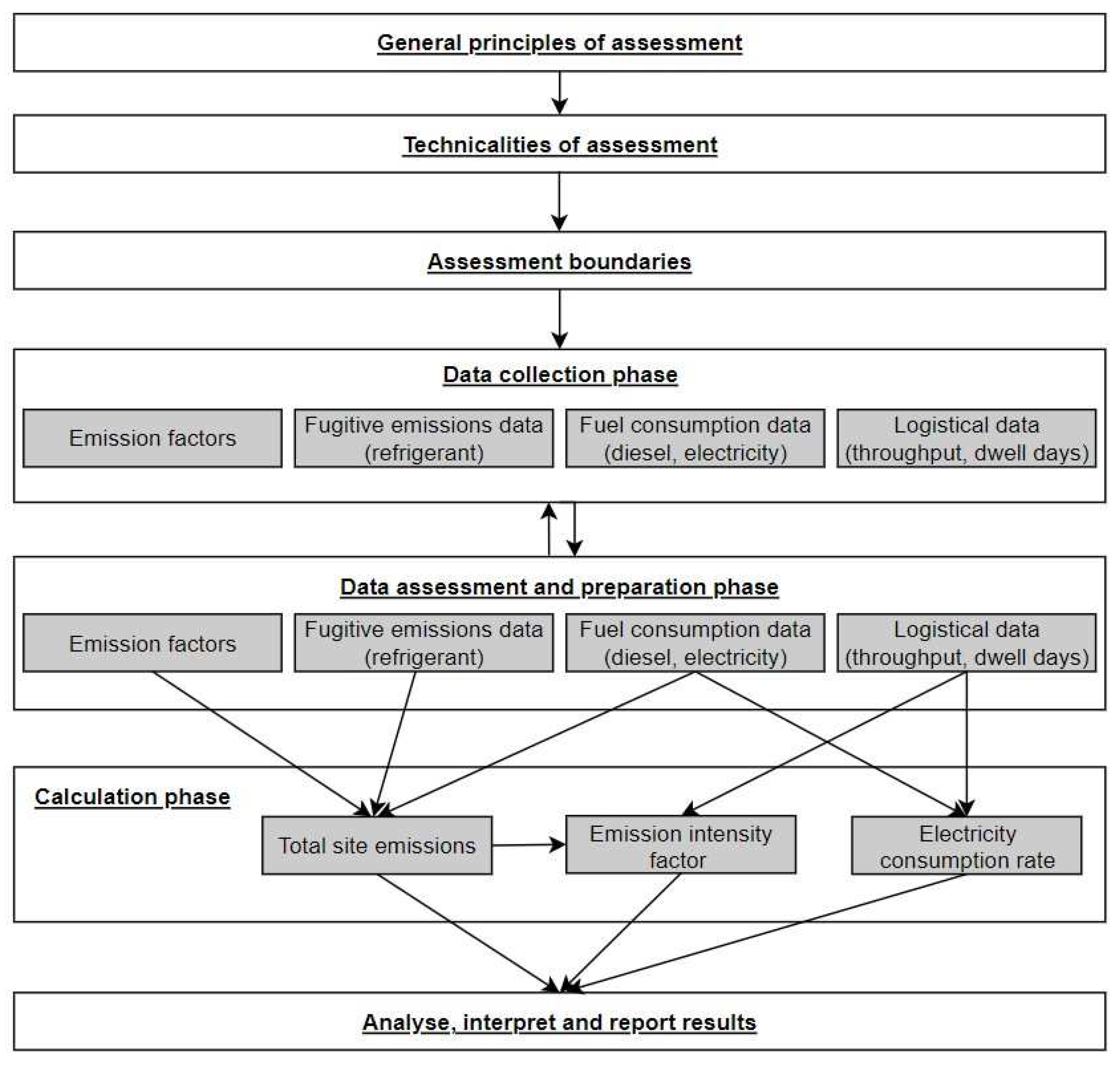
2. Research Methodology
2.1. General Principles of Assessment
- Scope 1 emissions: The emissions due to the burning of fuels, i.e., tank-to-wheel (TTW) in assets owned or controlled by the reporting company. Also included in this scope are the emissions due to refrigerant leakage from equipment at the reporting company’s plant.
- Scope 2 emissions: The indirect emissions due to purchased electricity by the reporting company.
- Scope 3, category 3 emissions: The indirect upstream emissions due to the extraction, production, and transportation of fuel and energy-related products that are not included in Scope 1 or Scope 2 emissions. This includes the upstream emissions of purchased fuels, i.e., well-to-tank (WTT) and the upstream emissions of purchased electricity, taking transmission and distribution losses into account. For a detailed discussion of calculating a reporting company’s category 3 emissions, refer to the WBCSD and WRI’s Technical Guidance for Calculating Scope 3 Emissions [29].
2.2. Technicalities of Assessment
2.2.1. Adjustments to Methodology
- In this assessment, the unit of analysis is pallets instead of the conventional tonne that is generally used in the emissions realm. According to Dobers et al. [20], the use of pallets as units of analysis is acceptable as long as these units are used throughout the assessment and allow for comparison of emissions over years. This means the resultant unit for emission intensity factors is kg CO2e pallet−1 instead of kg CO2e t−1. The reason for this adjustment is justified: all cold stores, fruit exporters, producers and stakeholders refer to pallets as the metric or functional unit after fruit has been packed and palletized and distribution commences. In addition, the pallet weight is often not captured by cold stores since this adds an added level of complexity to business operations and does not contribute any significant value. Using the consignment-based indicator (pallets) instead of the weight-based indicator (tonnes) still provides a consistent metric that is already in use. If the conversion between pallets and weight is required, the conversion factor of 1 030 kg pallet−1 can be used.
- The time duration of storage or dwell days directly affects the utilization percentage of the facility (i.e., how well the available capacity of the cold store is used). This, in turn, affects the emissions allocated to each pallet that moves through the facility. It is deemed essential to incorporate the time duration of storage in the assessment to provide an accurate and true representation of both the electricity consumption rate and emission intensity of storing a pallet. The time aspect is incorporated by either collecting the average dwell days of pallets from cold stores or by obtaining the average utilization percentage of the cold store. If neither of the two variables is available, a time-based element cannot be incorporated into the assessment. Refer to Section 3, Equation (2) for the conversion between dwell days and average utilization.
- Dobers et al. [20] suggest that emissions should be accounted for on an annual basis to remove seasonal effects. The authors are, however, of the opinion that the seasonal effect of different harvest seasons for different fruits must be assessed. Different fruit types, each with different refrigeration requirements and throughput volumes, are moved through a cold store during different months of the year. In addition, the effect of ambient temperature during different months of the year is also incorporated by performing the analysis on a monthly basis. However, to comply with Dobers et al. [20], the assessment and results of some facilities are done for both a monthly and an annual period.
2.2.2. Assumptions Required for Assessment
- The weight difference between fruit types and packaging configurations is negligible. This means all pallets of fruit have the same weight.
- All pallets have the same number of dwell days in a facility, independent of the type of fruit and the destination market.
- The energy consumed due to cold sterilization is apportioned to all pallets that move through the facility. The effect of fruit destined for different markets is therefore negligible.
- Pallets in the facility are all handled or processed in a comparable fashion, from offloading to storage to the eventual loading for shipment to the destination market.
- The energy effect of some fruits arriving at optimal storage temperature and others arriving above target temperature is allocated evenly among all pallets that move through the cold store.
- All fruit types and packaging configurations have the same cooling characteristics.
- The type of packaging has little to no effect on the energy efficiency and use of the cold store.
- The effect of fruit loss in any of the analyzed cold stores is ignored.
- Only the operational emissions or use-phase emissions of equipment and infrastructure are assessed.
- Leakage of refrigerants occurs in the same period that refilling with refrigerants occurs. Furthermore, the quantity of refrigerants refilled during a year is apportioned evenly between all months of the year.
2.3. Boundaries of Analysis
2.4. Data Collection
2.4.1. Cold-Store Consumption Data
2.4.2. Emission Factors (EF)
2.5. Data Assessment and Preparation Phase
3. Calculations
3.1. Total Site Emissions
- EmissionTotal = the total GHG emissions of the cold store for a period (kg CO2e)
- n = the total number of fuels (diesel, electricity or refrigerant) consumed
- Quantityi = the amount (ℓ, kWh or kg) of i used
- i = the type of fuel (diesel, electricity) or refrigerant used
- EFi = the emission factor for i (diesel, electricity or refrigerant) in (kg CO2e per unit).
3.2. Dwell Days or Utilisation
- Ddwell = the average number of dwell days a pallet spends in the facility (days)
- CapacityFacility = the total pallet capacity of the facility (pallets)
- DaysPeriod = the number of days in the analyzed period (days)
- UtilizAve = the average utilization of the facility in the time period (%)
- NPallets = the number of pallets moved during the analyzed time period (pallets)
3.3. Electricity Consumption Rate
- ElectricityPallet = the amount of electricity used per pallet-day (kWh pallet-d−1)
- Qelectricity = the total amount of electricity used by the cold store (kWh)
- Ddwell = the average dwell days a pallet spends in the facility (days) (Equation (2))
- NPallets = the number of pallets moved during the time period (pallets)
3.4. Diesel Consumption Rate
- ElectricityPallet = the amount of diesel used per pallet-day (ℓ pallet-d−1)
- Qdiesel = the total amount of diesel used by the cold store (ℓ)
- Ddwell = the average dwell days a pallet spends in the facility (days) (Equation (2))
- NPallets = the number of pallets moved during the time period (pallets)
3.5. Emission Intensity Factor
- EIFPallet = the average emission intensity factor for a pallet-day (kg CO2e pallet-d−1)
- EmissionTotal = the total GHG emissions of the cold store (kg CO2e)
- Ddwell = the average number of dwell days a pallet spends in the facility (days)
- NPallets = the number of pallets moved during the time period (pallets)
3.6. Average Values
- AveragePeriod = the average value for the period assessed
- Xi = the individual data values to be averaged
- n = the number of data values to be summed
- WeightedAve = the weighted average value
- n = the number of terms to be averaged in the calculation
- wi = the weight applied to each Xi value
- Xi = the data value to be averaged
4. Results
4.1. Seasonal Cold Stores
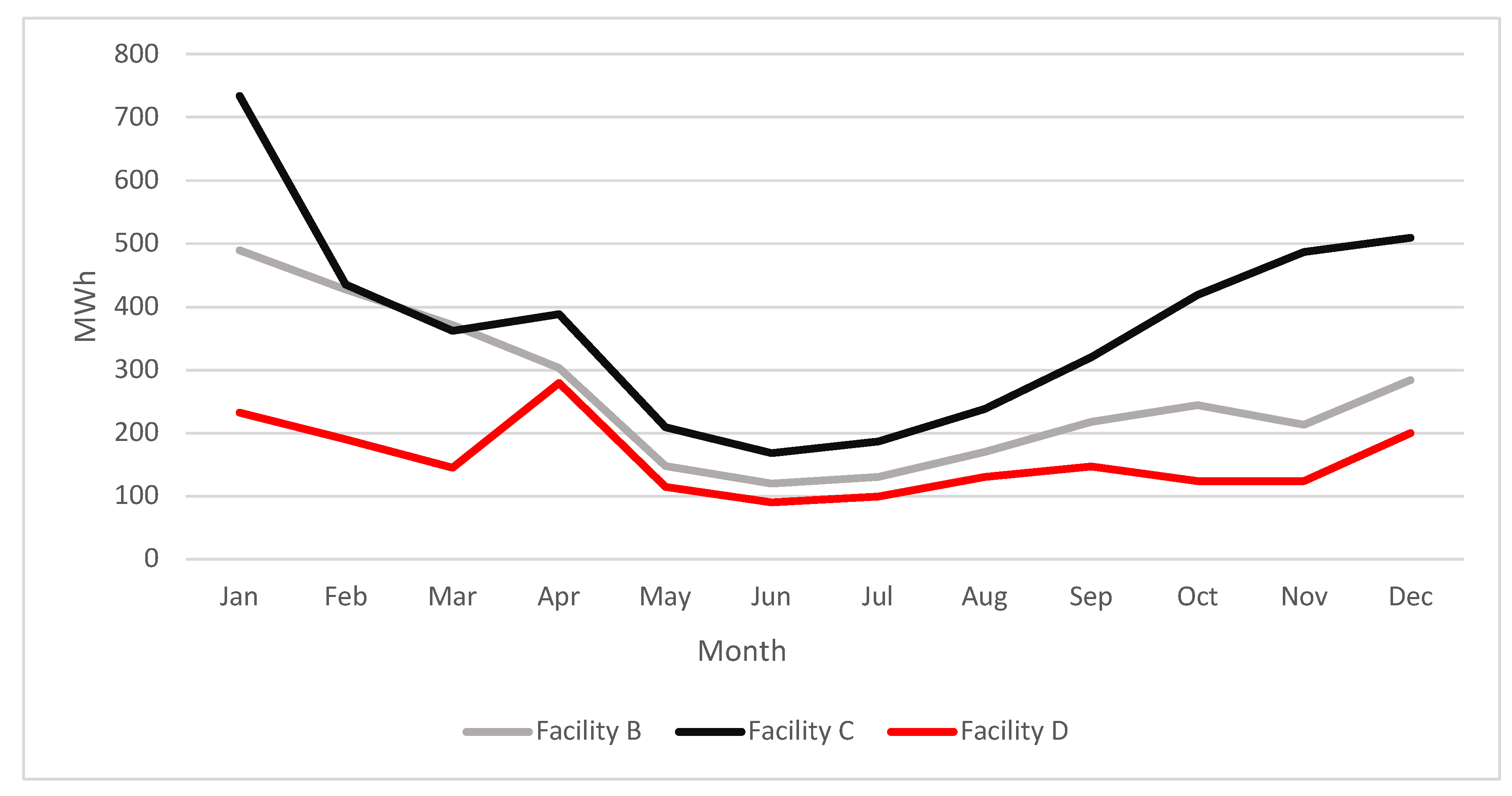
4.2. Large-Scale Commercial Facilities
4.2.1. Monthly Assessment Results
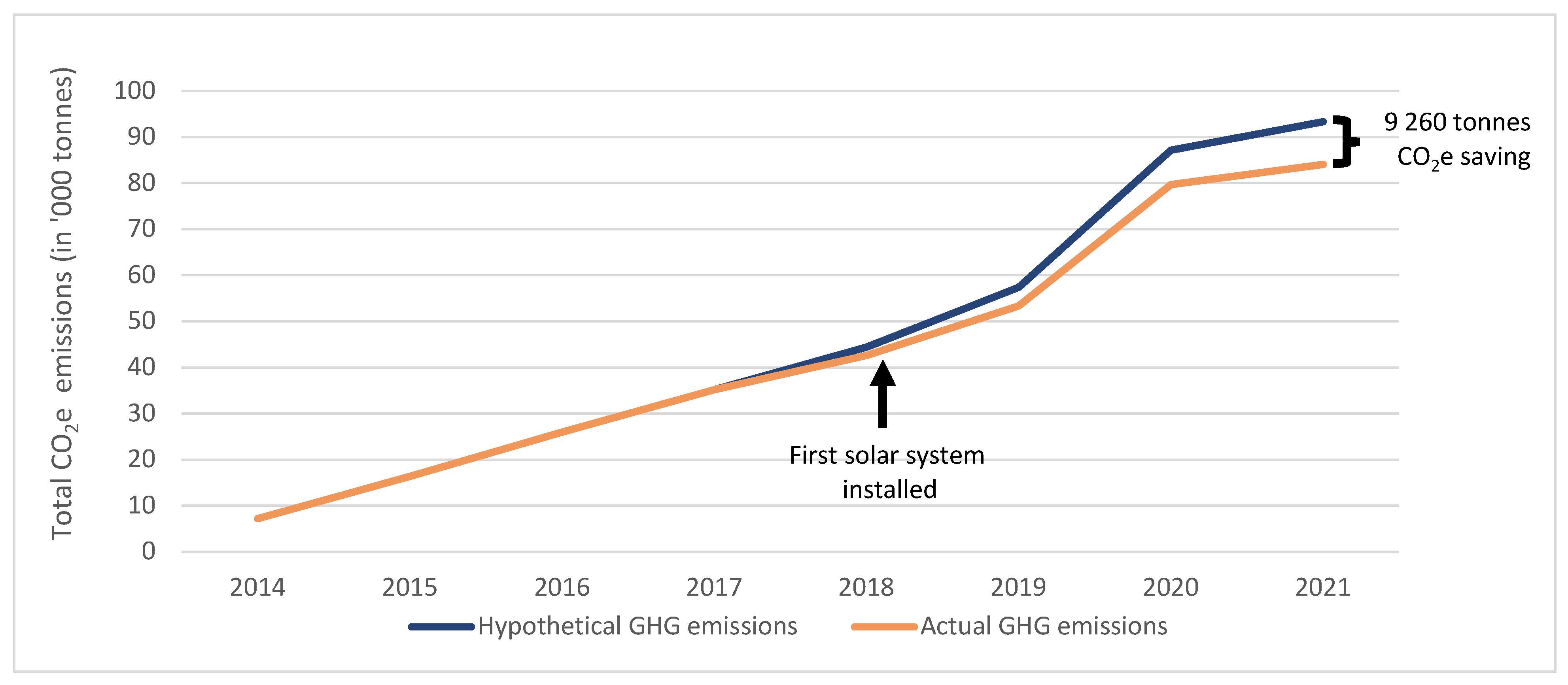
4.2.2. Annual Assessment Results
4.3. Cold Stores Regarded as Exceptions
5. Discussion
5.1. Sources of Emissions
5.2. Results
5.3. Reflection on Assessment
- Sensitive nature of organizational data: Due to the sensitive nature of organizational data, it is often difficult or impossible to obtain high-quality primary data. In the majority of cases, cold-store managers or other members of senior management are the only individuals who have access to the required data. These individuals are reluctant to share data for privacy reasons or due to a lack of understanding of the potential value of an assessment. In terms of the quality of data, some facilities do not record or keep records of all the required data for an emissions assessment. In some instances, as was the case for the diesel consumption at one of the cold stores in this study, the quantity of fuel used per month was not recorded and had to be derived from fuel invoices. This lack of quality data hampers emissions assessments since missing data cannot be substituted from literature, even if such data were available. Better capturing of the appropriate data elements mentioned in Section 2.4 is, therefore, required for more accurate assessments.
- A lack of a standard methodology for cold stores as logistical sites: There are still considerable research challenges with assessing, quantifying and gauging GHG emissions at a facility level, even when using the methodology developed by [20]. This lack of a prescriptive standard leaves room for erroneous assumptions and leads to both inaccurate and incomparable results.
- Allocation of emissions among logistical units: The process of fairly allocating the total emissions among all goods that moved through the cold store is a major problem (the allocation problem). The allocation of refrigeration energy should not only be fair but also practical to apply. Some shipments of fresh fruit are stored for a short duration and others for extended periods. The dwell days will certainly have an impact on the emissions value of a specific shipment. In addition to a time aspect, pallets of fruit have different configurations (prepared for standard or high-cube containers) or sizes, which lead to different weights.
- Dwell days and utilization: The number of dwell days and the utilization percentage of a facility have a major impact on the assessment results. Allocating emissions fairly to pallets that spend a couple of days in the cold store should be different to pallets that do so for weeks. The consumption rate of electricity (kWh pallet-d−1) and the emission intensity factor (kg CO2e pallet-d−1) are inversely related to the number of dwell days. If a time-based element is incorporated in an assessment, the dwell days must be accurate.
- Availability of emission factors: The accurate quantification of emissions is dependent on the availability of applicable emission factors, as stated in Section 2.5. Emission factors for fuels such as diesel are not available for South Africa. Since the feedstock and production process of fossil fuels differ from one geographical location to another, the emission factor could potentially be much higher in South Africa, particularly since South Africa’s fuel is partly derived from coal. If newer emission factors for South African electricity or diesel becomes available, the energy consumption in Table 3 can be multiplied by the new factors to provide a timelier hypothetical emission intensity factor.
6. Conclusions
Author Contributions
Funding
Institutional Review Board Statement
Informed Consent Statement
Data Availability Statement
Acknowledgments
Conflicts of Interest
Appendix A

| Parameters | |||
|---|---|---|---|
| Statistical Distribution | Location (μ) | Scale (σ) | |
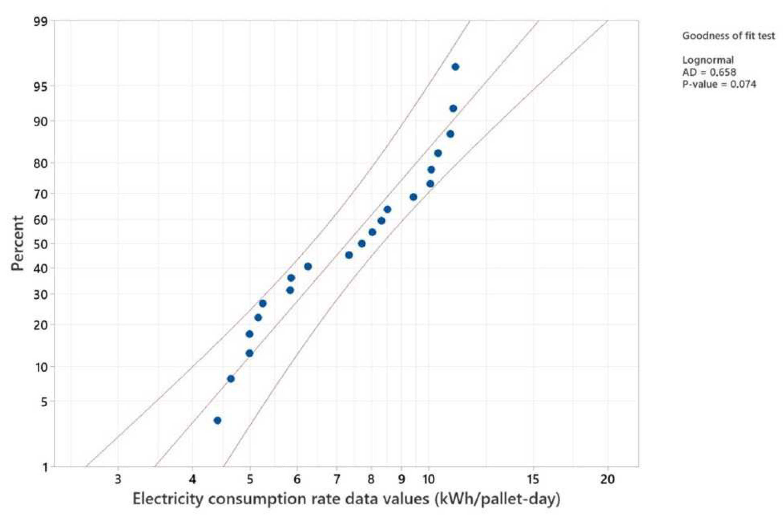
| Electricity consumption rate (kWh pallet-d−1) | Lognormal | 1.98360 | 0.32025 |
| Emission intensity factor (kg CO2e pallet-d−1) | Lognormal | 1.98360 | 0.32025 |


References
- UNCTAD. Global Trade Update—February 2022; Geneva: United Nations Conference on Trade and Development. 2022. Available online: https://unctad.org/system/files/official-document/ditcinf2022d1_en.pdf (accessed on 4 April 2022).
- Smart Freight Centre. Global Logistics Emissions Council Framework for Logistics Emissions Accounting and Reporting; Version 2.0; Smart Freight Centre: Amsterdam, The Netherlands, 2019; ISBN 978-90-82-68790-3. [Google Scholar]
- ITF. ITF Transport Outlook 2021; OECD Publishing: Paris, France, 2021; p. 14. [Google Scholar]
- Greenhouse Gas Emissions from Energy: Overview. Available online: https://www.iea.org/reports/greenhouse-gas-emissions-from-energy-overview/emissions-by-sector#abstract (accessed on 22 February 2022).
- Everything You Need to Know about the Fastest-Growing Source of Global Emissions: Transport. Available online: https://www.wri.org/insights/everything-you-need-know-about-fastest-growing-source-global-emissions-transport (accessed on 21 February 2022).
- WEF. Supply Chain Decarbonization—The Role of Logistics and Transport in Reducing the Supply Chain Carbon Emissions; World Economic Forum: Geneva, Switzerland, 2009. [Google Scholar]
- WEF. Net-Zero Challenge: The Supply Chain Opportunity; World Economic Forum: Geneva, Switzerland, 2021. [Google Scholar]
- Rüdiger, D.; Dobers, K.; Ehrler, V.; Lewis, A. Carbon Footprinting of Warehouses and Distribution Centers as Part of Road Freight Transport Chains. In Proceedings of the 4th International Workshop on Sustainable Road Freight Transport, Cambridge, UK, 30 November–1 December 2017; Fraunhofer IML: Dortmund, Germany, 2017. [Google Scholar]
- Higgins, C.D.; Ferguson, M.; Kanaroglou, P.S. Varieties of Logistics Centers. Transp. Res. Rec. J. Transp. Res. Board 2012, 2288, 9–18. [Google Scholar] [CrossRef]
- Lewis, A. Towards a Harmonized Framework for Calculating Logistics Carbon Footprint. In Sustainable Logistics and Supply Chains, 1st ed.; Lu, M., De Bock, J., Eds.; Springer: Cham, Switzerland, 2015; pp. 163–183. [Google Scholar]
- Supply Chain Resilience: How Are Pandemic-Related Disruptions Reshaping Managerial Thinking? Available online: https://www.weforum.org/agenda/2021/12/supply-chain-resilience-lessons-from-covid-19/ (accessed on 22 February 2022).
- Ries, J.M.; Grosse, E.H.; Fichtinger, J. Environmental Impact of Warehousing: A Scenario Analysis for the United States. Int. J. Prod. Res. 2017, 55, 6485–6499. [Google Scholar] [CrossRef]
- Rüdiger, D.; Schön, A.; Dobers, K. Managing Greenhouse Gas Emissions from Warehousing and Transshipment with Environmental Performance Indicators. Transp. Res. Procedia 2016, 14, 886–895. [Google Scholar] [CrossRef]
- Dobers, K.; Perotti, S.; Fossa, A. Emission Intensity Factors for Logistics Buildings; Fraunhofer IML: Dortmund, Germany, 2022. [Google Scholar]
- Mckinnon, A. Decarbonizing Logistics: Distributing Goods in a Low-Carbon World, 1st ed.; Kogan Page: London, UK, 2018; p. 14. [Google Scholar]
- Dhooma, J.; Baker, P. An Exploratory Framework for Energy Conservation in Existing Warehouses. Int. J. Logist. Res. Appl. 2012, 15, 37–51. [Google Scholar] [CrossRef]
- Dobers, K.; Ehrler, V.C.; Davydenko, I.Y.; Rüdiger, D.; Clausen, U. Challenges to Standardizing Emissions Calculation of Logistics Hubs as Basis for Decarbonizing Transport Chains on a Global Scale. Transp. Res. Rec. 2019, 2673, 502–513. [Google Scholar] [CrossRef]
- du Plessis, M.; van Eeden, J.; Goedhals-Gerber, L. Carbon mapping frameworks for the distribution of fresh fruit: A systematic review. Glob. Food Sec. 2022, 32, 100607. [Google Scholar] [CrossRef]
- Lewczuk, K.; Kłodawski, M.; Gepner, P. Energy consumption in a distributional warehouse: A practical case study for different warehouse technologies. Energies 2021, 14, 2709. [Google Scholar] [CrossRef]
- Dobers, K.; Rüdiger, D.; Jarmer, J.P. Guide for Greenhouse Gas Emissions Accounting for Logistic Sites, 1st ed.; Die Deutsche Nationalbibliothek: Stuttgart, Germany, 2019; pp. 9–63. [Google Scholar]
- Falagán, N.; Terry, L.A. Recent Advances in Controlled and Modified Atmosphere of Fresh Produce. Johns. Matthey Technol. Rev. 2018, 62, 107–117. [Google Scholar] [CrossRef]
- du Plessis, M.J.; van Eeden, J.; Goedhals-Gerber, L.L. Distribution Chain Diagrams for Fresh Fruit Supply Chains: A Baseline for Emission Assessment. J. Transp. Supply Chain Manag. 2022. [Google Scholar] [CrossRef]
- WBCSD; WRI. The Greenhouse Gas Protocol: A Corporate Accounting and Reporting Standard, Revised ed.; World Business Council for Sustainable Development, World Resource Institute: Washington, DC, USA, 2004. [Google Scholar]
- Iriarte, A.; Yáñez, P.; Villalobos, P.; Huenchuleo, C.; Rebolledo-Leiva, R. Carbon Footprint of Southern Hemisphere Fruit Exported to Europe: The Case of Chilean Apple to the UK. J. Clean. Prod. 2021, 293, 126118. [Google Scholar] [CrossRef]
- South Africa Again Exports More Fruit in 2021; Mandarin Exports 30% Higher. Available online: https://www.freshplaza.com/article/9385397/south-africa-again-exports-more-fruit-in-2021-mandarin-exports-30-higher/ (accessed on 5 April 2022).
- Fresh Produce Exporters Forum. Fresh Produce Export Directory 2021; Fresh Produce Exporters Forum: Cape Town, South Africa, 2021. [Google Scholar]
- Eskom. Integrated Report—2021; Eskom Holdings SOC Ltd.: Johannesburg, South Africa, 2021. [Google Scholar]
- Eskom. Eskom Factor 2.0; Eskom Holdings SOC Ltd.: Johannesburg, South Africa, 2018. [Google Scholar]
- WBCSD; WRI. Technical Guidance for Calculating Scope 3 Emissions; Version 1; Greenhouse Gas Protocol: Online, 2013. [Google Scholar]
- BSI BS EN 16258:2012; Methodology for Calculation and Declaration of Energy Consumption and GHG Emissions of Transport Services (Freight and Passengers). 2012th ed. BSI Standards Limited: London, UK, 2012; ISBN 978-0-580-74301-6.
- IPCC. Climate Change 2007: The Physical Science Basis. Contribution of Working Group I to the Fourth Assessment Report of the Intergovernmental Panel on Climate Change; Cambridge University Press: Cambridge, UK; New York, NY, USA, 2007. [Google Scholar]
- DALRRD. Fresh Food Trade SA, 9th ed.; Department of Agriculture, Land Reform and Rural Development: Pretoria, South Africa, 2021.


| Type of Logistical Site | Ambient (kg CO2e t−1) | Mixed (kg CO2e t−1) | Chilled (kg CO2e t−1) |
|---|---|---|---|
| Transshipment | 3.4 | 3.8 | 11.1 |
| Storage and transshipment | 1.7 | 12.3 | 7.3 |
| Warehouse (storage) | 1.9 | 8.9 | 8.2 |
| Electricity | Diesel | Refrigerant Data | Logistical Data |
|---|---|---|---|
| Total amount of grid electricity (kWh) used | Total amount of diesel (ℓ) used at the facility by generators and/or equipment | Types of refrigerants used at the facility | Pallet capacity of facility |
| Total amount of electricity generated (kWh) by solar panels | Refrigerant capacity of all systems (kg) | Total throughput at the facility (number of pallets) | |
| Total refill values of refrigerants (kg) | Average dwell days or utilization percentage of the facility |
| Dwell Days | |||||||
|---|---|---|---|---|---|---|---|
| 1 | 2 | 3 | 4 | 5 | 6 | 7 | |
| Electricity consumption rate (kWh pallet-d−1) 1 | 57.49 | 28.75 | 19.16 | 14.37 | 11.50 | 9.58 | 8.21 |
| Diesel consumption rate (ℓ pallet-d−1) | 0.20 | 0.10 | 0.07 | 0.05 | 0.04 | 0.03 | 0.03 |
| Emission intensity factor (kg CO2e pallet-d−1) | 56.99 | 28.50 | 19.00 | 14.25 | 11.40 | 9.50 | 8.14 |
| Utilization percentage of facility | 8.95% | 17.89% | 26.84% | 35.79% | 44.73% | 53.68% | 62.63% |
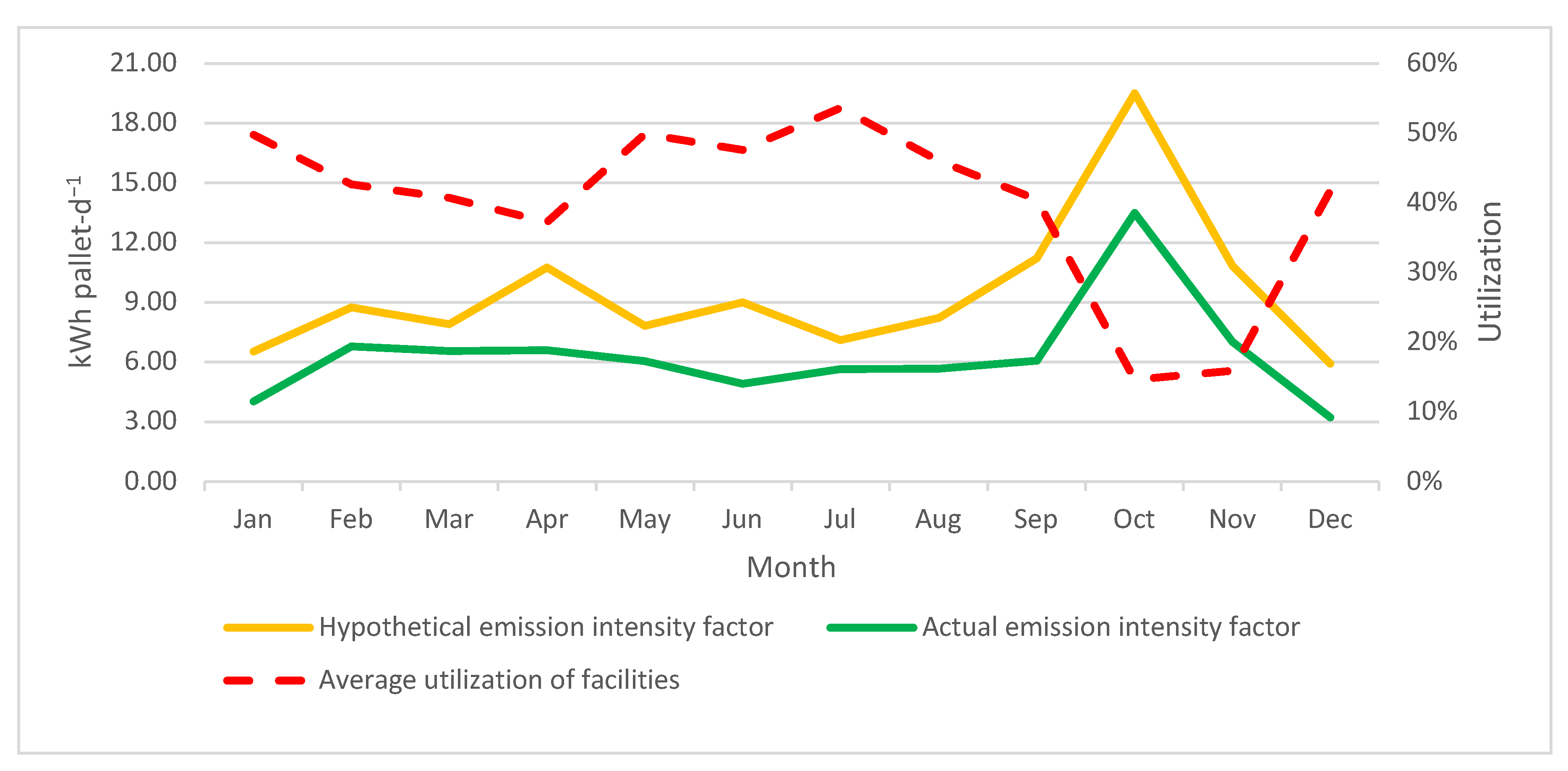
| Jan | Feb | Mar | Apr | May | Jun | Jul | Aug | Sep | Oct | Nov | Dec | |
|---|---|---|---|---|---|---|---|---|---|---|---|---|
| Electricity consumption rate (kWh pallet-d−1) 1 | 6.62 | 8.87 | 8.01 | 10.92 | 7.92 | 9.16 | 7.21 | 8.35 | 11.41 | 19.77 | 10.94 | 5.90 |
| Diesel consumption rate (ℓ pallet-d−1) | 0.02 | 0.02 | 0.02 | 0.02 | 0.02 | 0.01 | 0.01 | 0.01 | 0.02 | 0.05 | 0.05 | 0.05 |
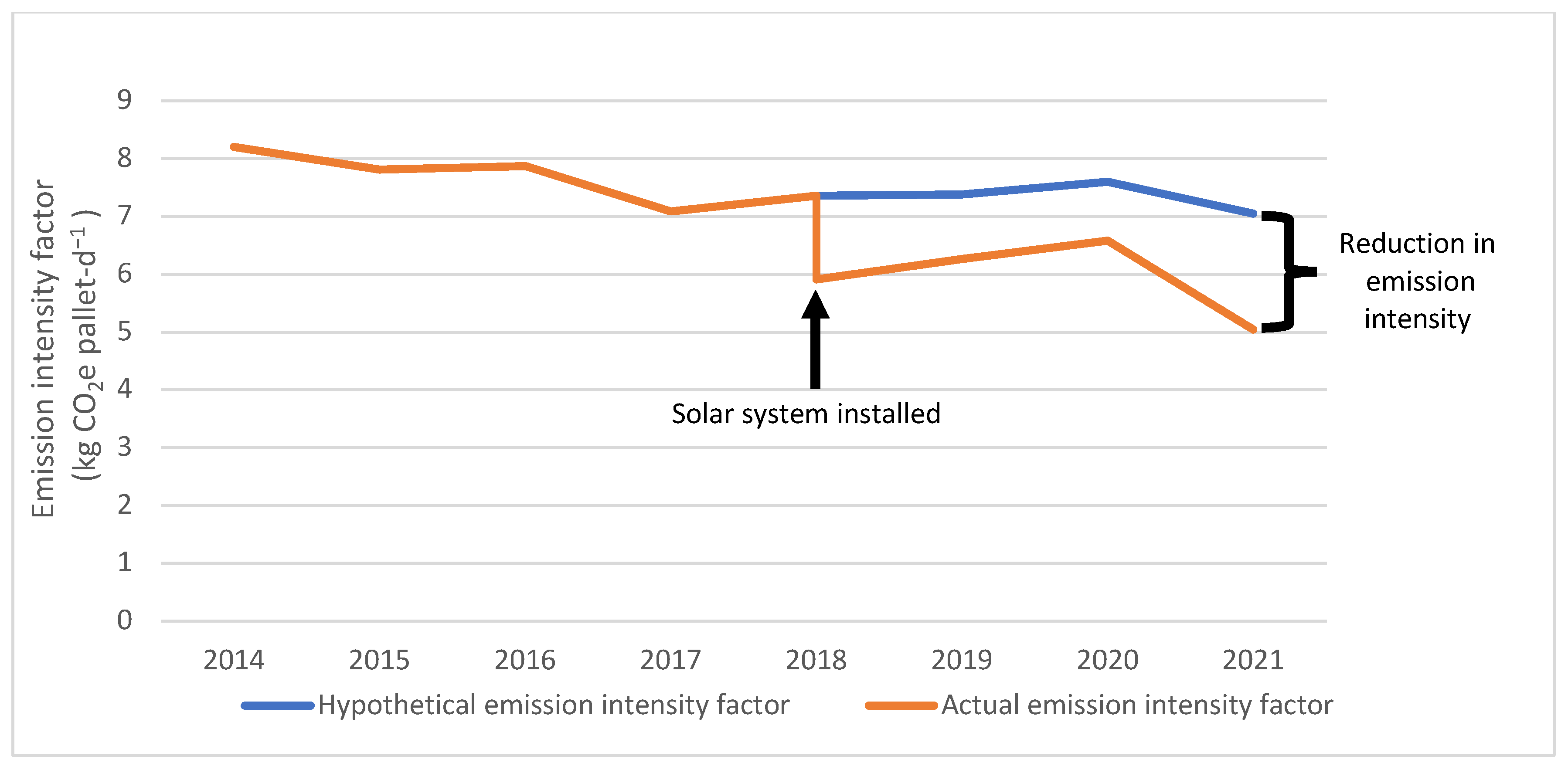
| Hypothetical emission intensity factor— assuming no solar (kg CO2e pallet-d−1) | 6.52 | 8.74 | 7.91 | 10.74 | 7.81 | 9.00 | 7.09 | 8.20 | 11.22 | 19.49 | 10.82 | 5.92 |
| Actual emission intensity factor—with solar (kg CO2e pallet-d−1) | 4.03 | 6.78 | 6.55 | 6.60 | 6.05 | 4.91 | 5.64 | 5.67 | 6.06 | 13.49 | 7.02 | 3.22 |
| Utilization percentage of facility | 49.74% | 42.63% | 40.70% | 37.23% | 49.83% | 47.60% | 53.62% | 46.02% | 40.49% | 14.64% | 15.86% | 41.73% |
| Average Annual Value | |
|---|---|
| Electricity consumption rate (kWh pallet-d−1) 1 | 7.62 |
| Diesel consumption rate (ℓ pallet-d−1) | 0.014 |
| Hypothetical emission intensity factor— assuming no solar (kg CO2e pallet-d−1) | 7.52 |
| Actual emission intensity factor— with solar (kg CO2e pallet-d−1) | 5.72 |
| Utilization percentage of facility | 40.25% |
| Jan | Feb | Mar | Apr | May | Jun | Jul | Aug | Sep | Oct | Nov | Dec | |
|---|---|---|---|---|---|---|---|---|---|---|---|---|
| Electricity consumption rate (kWh pallet-d−1) 1 | 20.51 | 34.27 | 12.92 | 8.74 | 8.10 | 7.74 | 7.75 | 10.56 | 13.83 | 47.12 | 32.12 | 9.63 |
| Emission intensity factor (kg CO2e pallet-d−1) | 20.10 | 33.58 | 12.67 | 8.57 | 7.93 | 7.59 | 7.59 | 10.35 | 13.55 | 46.18 | 31.48 | 9.44 |
| Utilization percentage of facility | 30.22% | 18.16% | 37.98% | 57.83% | 55.13% | 52.24% | 52.12% | 43.07% | 33.79% | 9.41% | 13.77% | 31.07% |
| Jan | Feb | Mar | Apr | May | Jun | Jul | Aug | Sep | Oct | Nov | Dec | |
|---|---|---|---|---|---|---|---|---|---|---|---|---|
| Electricity consumption rate (kWh pallet-d−1) 1 | 24.54 | 25.82 | 17.79 | 12.73 | 5.40 | 4.07 | 3.02 | 2.96 | 4.11 | 23.89 | 24.46 | 33.24 |
| Fugitive emissions (kg CO2e pallet-d−1) | 75.47 | 64.31 | 58.43 | 44.14 | 9.34 | 5.22 | 3.12 | 2.17 | 7.13 | 36.22 | 43.03 | 49.88 |
| Emission intensity factor (kg CO2e pallet-d−1) | 99.52 | 89.61 | 75.87 | 56.62 | 14.64 | 9.21 | 6.08 | 5.07 | 11.16 | 59.63 | 67.01 | 82.46 |
| Utilization percentage of facility | 9.45% | 8.33% | 8.76% | 19.34% | 46.42% | 61.40% | 84.24% | 96.12% | 51.67% | 13.37% | 15.21% | 13.98% |
Publisher’s Note: MDPI stays neutral with regard to jurisdictional claims in published maps and institutional affiliations. |
© 2022 by the authors. Licensee MDPI, Basel, Switzerland. This article is an open access article distributed under the terms and conditions of the Creative Commons Attribution (CC BY) license (https://creativecommons.org/licenses/by/4.0/).
Share and Cite
du Plessis, M.J.; van Eeden, J.; Goedhals-Gerber, L.L. The Carbon Footprint of Fruit Storage: A Case Study of the Energy and Emission Intensity of Cold Stores. Sustainability 2022, 14, 7530. https://0-doi-org.brum.beds.ac.uk/10.3390/su14137530
du Plessis MJ, van Eeden J, Goedhals-Gerber LL. The Carbon Footprint of Fruit Storage: A Case Study of the Energy and Emission Intensity of Cold Stores. Sustainability. 2022; 14(13):7530. https://0-doi-org.brum.beds.ac.uk/10.3390/su14137530
Chicago/Turabian Styledu Plessis, Martin Johannes, Joubert van Eeden, and Leila Louise Goedhals-Gerber. 2022. "The Carbon Footprint of Fruit Storage: A Case Study of the Energy and Emission Intensity of Cold Stores" Sustainability 14, no. 13: 7530. https://0-doi-org.brum.beds.ac.uk/10.3390/su14137530