1. Introduction
Performance of pavement structures, which comprise surface, base and subgrade layers, depends on the behavior of all these layers. Nevertheless, Schwartz et al. [
1] stated that the performance anticipated by the American Association of State Highways and Transportation Officials Ware (AASHTOWare) Pavement Mechanistic-Empirical (ME) Design shows low or no sensitivity to inputs from unbound layers and subgrade. Furthermore, they found that total rutting in flexible pavements had only marginal sensitivity to the resilient modulus of subgrade and non-sensitivity to the thickness of the unbound layer.
Total rutting, which is a major failure mode of flexible pavements, is mainly caused by the permanent deformation of the pavement layers along a wheel path that affects the riding quality and structural health of these pavements. Based on the local calibration of the mechanistic-empirical pavement design guide (MEPDG) rutting models for flexible pavements, Waseem and Yuan [
2] suggested a percentage of contributions of different pavement layers to total rutting. Orobio and Zaniewski [
3] found that the resilient modulus of subgrade notably affects the rutting predicted by MEPDG. Based on the MEPDG prediction model, Baus and Stires [
4] found that the resilient modulus of subgrade significantly influences pavement roughness, total rutting, alligator cracking and longitudinal cracking for a number of pavements in South Carolina. Thus, subgrade soil appears to have remarkable effects on the accumulation of different types of distress in flexible pavements. Nevertheless, the resilient modulus did not fully account for rutting or permanent deformation of subgrade because it reflects elastic behavior that is directly linked to recoverable deformation while rutting is a result of irrecoverable plastic deformation. For example, soils such as silts exhibit moderate to high resilient moduli while generating large permanent deformations under repeated loading, thus illustrating why resilient modulus of subgrade is not always the best measure of rutting. In addition, direct subgrade strength parameter is not included in the MEPDG rut prediction model [
5]. Puppala et al. [
6] formulated a four-parameter permanent strain model formulation, which is based on multiple nonlinear regression analysis to predict rutting or permanent strains in various soils. They believed this model provided additional information on whether subgrades experience excessive rutting under cyclic loads, and that it should be included in the flexible pavement design along with the characterization of resilient properties of subgrade soils.
Pavement performance models provide prediction of future pavement performance based on the known present or past pavement conditions along with the data containing the variables that control the pavement deterioration. These models provide very valuable tool for rational allocation of resources at the network level [
7], thus resulting in more money savings [
8]. Performance models have been developed by several states in the USA and worldwide. Johnson and Cation [
9] developed a pavement performance model for the North Dakota Department of Transportation (NDDOT) by using a roughness index, distress index and structural index. Chan et al. [
10] developed a pavement performance model for the North Carolina Department of Transportation (NCDOT) based on the pavement condition rating. The model included alligator cracking, edge cracking, block/transverse cracking, reflective cracking, rutting, raveling, bleeding, ride quality and patching. DeLisle et al. [
11] developed a network level performance model by using the 20 years of historical data for pavements in the state of New York. The corresponding data are based entirely on the extent of cracking on the pavement surface. Prozi and Madanat [
12] developed pavement performance models for pavements in Minnesota by using regression techniques and data from AASHTO road test. The riding quality of the different parts was tracked by monitoring the serviceability expressed as the present serviceability index (PSI) that is based on the data containing the road’s longitudinal roughness, patch work, rutting and cracking. Kim and Kim [
13] found linear regression models to be an effective predictor of pavement performance expressed in terms of rutting, cracks, patches, etc. Mills et al. [
14] used simple and multiple regression models to predict pavement performance in Delaware in terms of cracks and patches. Henning et al. [
15] used data from long-term pavement performance (LTPP) sites to calibrate pavement performance models in New Zealand based on distresses such as rutting, cracks and roughness. Isa et al. [
16] used regression techniques to develop pavement performance models for federal roads in Malaysia based on rutting and roughness.
Rahman et al. [
17] performed a statistical analysis through multiple linear regression techniques to develop estimation models for resilient modulus (
MR) of undisturbed soils using soils index properties. Rahman et al. [
18] developed performance evaluation models for asphalt concrete (AC) pavements and jointed-plain concrete pavements (JPCP) using multiple regression techniques for different distress indicators including PSI, pavement distress index (PDI), pavement quality index (PQI), and international roughness index (IRI). Osorio-Lird et al. [
19] proposed a methodology for the development of urban pavement performance models based on probabilistic trends observed from field evaluations applying Markov chains and Monte Carlo simulation.
In addition, statistical analyses were recently used to assess the effects of various improvement techniques on rutting. Qadir et al. [
20] investigated the effects of flexible and rigid geogrid materials in asphalt pavement on the resistance to rutting through analysis of variance (ANOVA) and multivariate linear regression (MLR) that were used for comparison and modeling, respectively. Ismael et al. [
21] studied effects of carbon nanotube (CNT) additives on the resistance of asphalt pavement to rutting. They conducted statistical analysis based on all obtained data to establish the model that involved the main mixtures variables. The stepwise technique produced a regression model that correlated the vital role of CNT presence to the rutting resistance. Zachariah et al. [
22] studied the moisture damage and rutting resistance of polypropylene modified bituminous mixes with crushed brick aggregate wastes. ANOVA with a 95% confidence level was also performed on the results to study the effect of variables on the rutting resistance and moisture susceptibility.
In addition to statistical approach, finite element (FE) modeling has also been used for prediction and analysis of pavement distresses. For example, Shanbara et al. [
23] performed 3D finite element simulations of small-scale laboratory wheel tracking tests that were conducted on cold-mix asphalt (CMA) pavements. The main goal was to capture the rutting response of both, unreinforced pavements and pavements reinforced with coir and jute fibers. CMA was modeled as a viscoelastic material while no subgrade was included either in the experiment or in the computational model. While the agreement between the predictions of computational model and experimental data was very good at 45 °C it deteriorated with increase in the pavement temperature. Alimohammadi et al. [
24] performed 2D FE simulations of a Hamburg wheel tracking test that is another small-scale laboratory test. They modeled hot-mix asphalt (HMA) and warm-mix asphalt (WMA) as viscoelastic materials and no subgrade was included either in the experiment or in FE model. The agreement between predictions of evolution of permanent deformation with number of passes varied with type of HMA/WMA used whereby some predictions were very good. Al-Rub et al. [
25] conducted 2D and 3D finite element simulations of a small-scale laboratory wheel-tracking test. They compared effects of different loading modes on evolution of rutting while no experimental data were included. They also investigated the effects of different material types on evolution of rutting including: (1) viscoelastic-viscoplastic, (2) elastic-viscoplastic and (3) coupled viscoelastic, viscoplastic and viscodamage models. No subgrade was included in the models. Lu and Hajj [
26] employed 3D finite element simulations to investigate the response of asphalt pavement sections with and without patches to load. Performances of different sizes and shapes of patches were compared. Asphalt was modeled as viscoelastic material and no experimental data were included.
Objectives and Scope
The main objective of this study was to evaluate the effects of subgrade and unbound layer on the performance of flexible pavements in Kansas, USA. To accomplish this objective the relevant data, which were collected over several years from 21 pavement segments located throughout state of Kansas, were used. The data contain information about major types of pavement distress along with the information about subgrade, unbound layer and traffic. Based on the amount of data available and objectives of this study the statistical approach was deemed the most appropriate.
The additional objective included providing recommendation for the selection of an acceptable California bearing ratio (
CBR) value, based on the results obtained from the statistical analyses.
CBR values were obtained by converting the results of in situ dynamic cone penetrometer (DCP) tests, which were conducted on subgrade soils, to corresponding
CBR values according to the statistical correlation [
27].
According to Siekmeier et al. [
28], the stated DCP test is a performance-related construction quality assurance test that is expected to increase uniformity of compaction and lower the life cycle maintenance costs. Thus, besides providing the relevant information about subgrade soils, using DCP test results as input into pavement performance prediction models most probably leads to improved resilience and increased sustainability of pavements that is achieved through decreased maintenance costs and decreased carbon footprint.
2. Development of Pavement Performance Prediction Models
Effects of subgrade and unbound layer on performance of flexible pavements in Kansas were evaluated by developing pavement performance prediction models based on the data that contain key indicators of the past performance. This approach was selected because it was deemed capable of providing statistical interdependencies between the causes of pavement distress and typical measures of the pavement distress whereby the selected causes primarily convey the information about subgrade and unbound layer. Furthermore, it was thought that the discovered interdependencies would provide the basis for determining the acceptable value of CBR for flexible pavements in Kansas.
Luo et al. [
29] conducted a study addressing mechanistic-empirical models for better consideration of the influence of subgrade and unbound layers on pavement performance. They pointed out that important factors affecting pavement performance include material properties, material behaviors, structural conditions, traffic and environment. Furthermore, Luo et al. [
29] selected rutting, fatigue cracking, transverse cracking and pavement roughness to characterize the distresses of flexible pavements. Consequently, the output variables or indicators of flexible pavement performance selected herein are: (1) total rutting, (2) fatigue cracking, (3) transverse cracking, (4) pavement roughness and (5) quality of pavement cores. The selected input variables are: (1) DCP tests conducted on subgrade soils in depths ranging from 0 to 0.32 m, (2) traffic volume data in the form of average annual daily truck traffic (AADTT) and (3) the thickness of unbound layer (
Th).
2.1. Input Data
Pavement conditions in Kansas were evaluated based on pavement roughness and surface distress data that were collected by DPI (KDOT). According to the recommendation of Baus and Stires [
4], who suggested using at least 20 pavement segments for calibrating and validating pavement distress conditions, 21 pavement segments were selected in the present study.
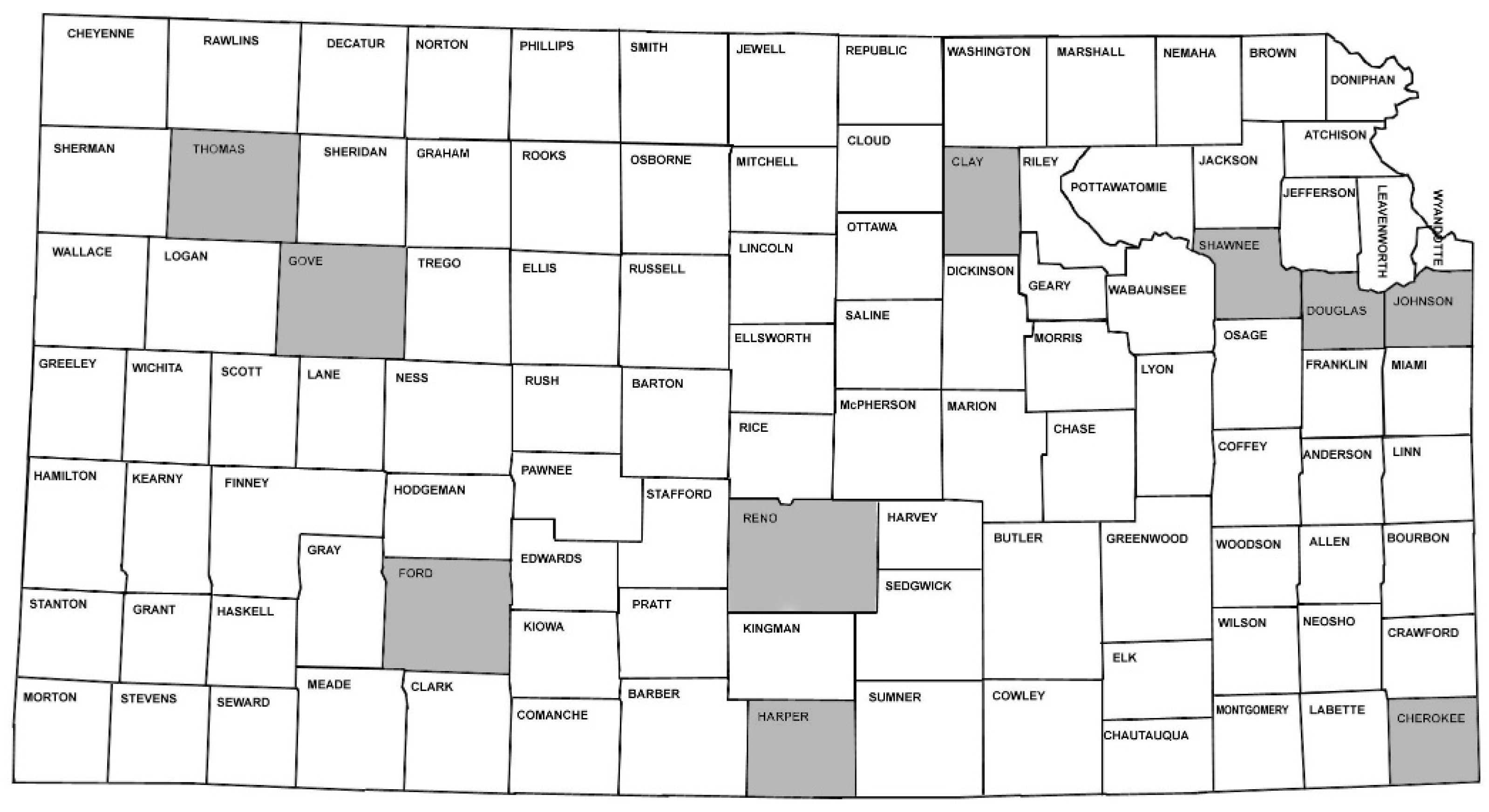
Table 1 provides locations of the selected flexible pavement segments whereby EB and WB denote eastbound and westbound lanes, respectively, while NB and SB denote northbound and southbound lanes, respectively. In addition,
Table 1 contains thicknesses of unbound layers, year in which DCP tests were performed and the year of the last pavement treatment. Geographic location of the counties, within which the selected pavement segments are located, is depicted in
Figure 1. Thus, diverse locations across the state of Kansas were included including east, west, north and south. The data reflecting pavements performance since the last pavement treatment were used herein.
DCP test assesses the structural capacity of a subgrade [
30]. It is because it can assess the amount and uniformity of subgrade compaction that it is an excellent quality control tool [
31,
32]. DCP test results have been correlated with engineering properties, such as elastic modulus, shear strength and
CBR test [
33,
34]. The advantages of DCP include low investment costs, portability and capability for rapid testing of subgrades and pavement layers. The test can be conducted within 15 min, thus providing reliable estimates of the corresponding
CBR values [
35].
The DCP tests for the selected pavement sections were conducted in three-year period from 2014 to 2017. The average time difference between the last treatment and the year in which DCP tests were conducted is 4.36 years. DCP tests were conducted on subgrade soils after extracting pavement cores. DCP test measures the resistance of in-situ soil against dynamic penetration. The test is performed by driving metal cone into the soil by striking it with 78.28 N weight dropped from a distance of 0.688 m. The penetration of the cone after each blow is checked and recorded in order to provide continuous measurements versus depth. DCP results herein are reported in terms of DCP penetration index (DPI), which is expressed in mm/below versus depth. The KDOT geotechnical manual states that DCP results from two top 0.152 m interval should be converted to CBR. In this study, DCP results from top 0.32 m of subgrade were used.
KDOT provided the Equation (1) based on which the current AADTT can be estimated. It is given by:
where
TTVGR is truck traffic volume growth rate,
AADTTcurrent is AADTT in the current year and
AADTTinitial is AADTT in the initial map year. Additional data were provided for all selected pavement sections including the initial map year and corresponding AADTT, as well as AADTT in the year when DCP tests were conducted. Based on this information
TTVGR can be computed and thus AADTT in any year of interest can be calculated. The average AADTT since the last pavement treatment was used as an input into statistical analyses for Clay County. The average value was computed based on AADTT values for years 2012, 2013 and 2014.
The data for pavement layers that are present in all pavement segments selected for the statistical analyses were provided by KDOT, including the thickness of unbound layer (
Table 1).
2.2. Output Data
Beginning in 2013, all flexible pavement condition data were collected through an automated system that collects pavement intensity and range images. South Dakota Profilometer with laser sensors was used to collect data for this study. The pavement distress indicators used in this study include: (1) total rutting, (2) fatigue cracking, (3) transverse cracking, (4) roughness and (5) core analysis. Most of data reflecting pavement distress in this study were available only in the form of distress indicator codes. Nevertheless, it is noted that although use of distress indicator codes is simple and good for pavement management system it may not be the most appropriate for performance prediction models as it does not provide very detailed information.
2.2.1. Total Rutting
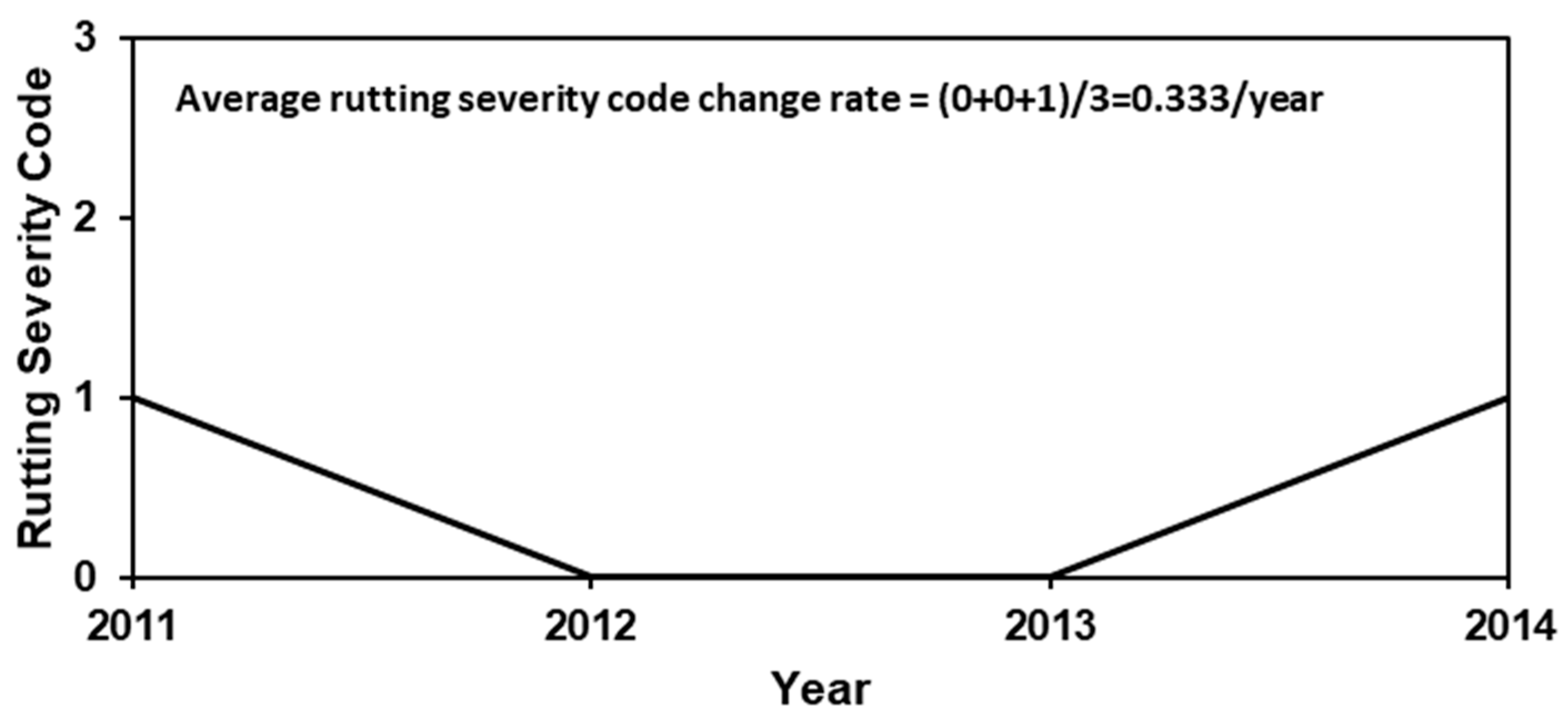
Rutting is a longitudinal surface depression along the wheel path. Total rutting (Rt) is a result of permanent deformation in each pavement layer. KDOT reports it in terms of rutting severity codes zero (0), one (1), two (2) and three (3) that correspond to rut depths of 0 to 6.3 mm, 6.3 to 12.7 mm, 12.7 to 25.4 mm and larger than 25.4 mm, respectively. Rutting codes of two and three are flagged as “Rutting” and “RUTTING”, respectively, while the rut depth of less than 12.7 mm is considered as less severe [
36].
Figure 2 depicts the evolution of the rutting severity code since the last pavement treatment for Clay County. Thus, the average rate of the change of rutting severity code since the last treatment is 0.333/year.
2.2.2. Fatigue Cracking
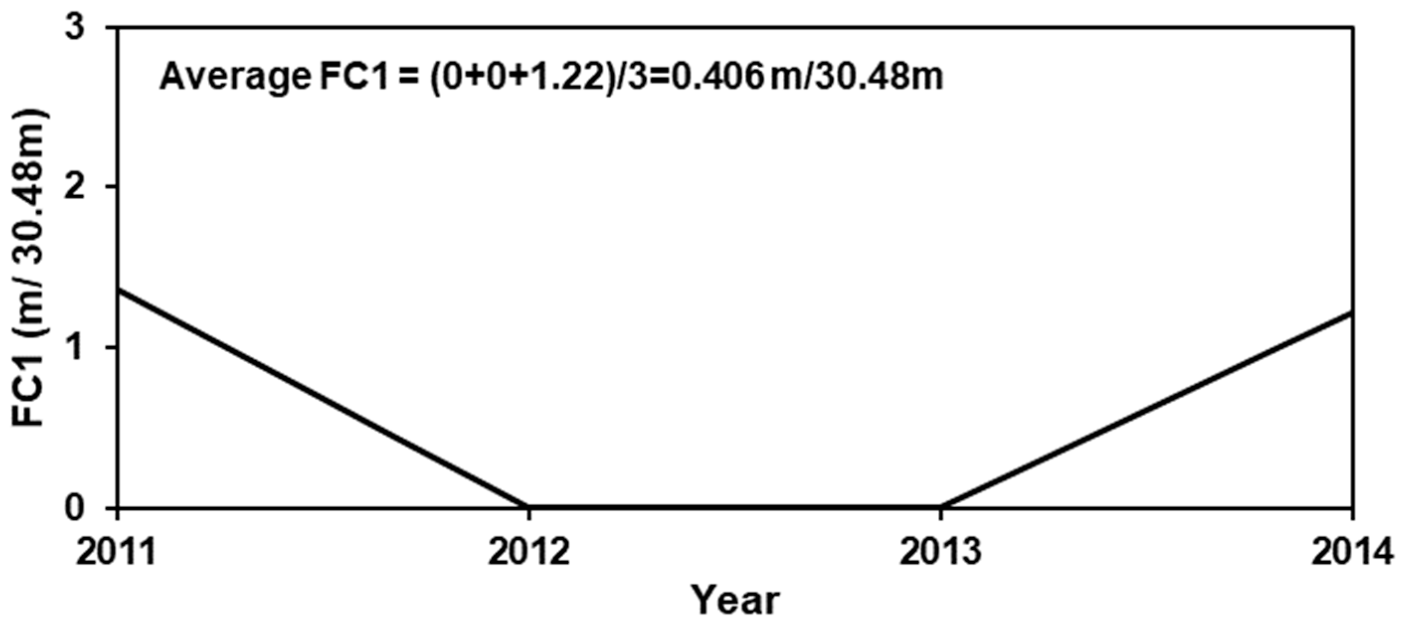
Fatigue cracking is expressed in lineal meter of fatigue cracking per 30.48 m sample. It is categorized as codes one (FC1), two (FC2), three (FC3) and four (FC4). Code one describes hairline alligator cracking with non-removable pieces. Code two corresponds to alligator cracking with spalled cracks and non-removable pieces. Code three describes alligator cracking with loose and removable pieces while pavement might pump. Code four describes the pavement that has shoved, thus forming a ridge of material adjacent to the wheel path. KDOT pavement management information systems (PMIS) provided the definitions of different fatigue cracking codes. The evolution of FC1 since the last pavement treatment for Clay County is depicted in
Figure 3. The corresponding average rate of change of FC1 since the last treatment is 0.406 m/30.48 m/year.
2.2.3. Transverse Cracking
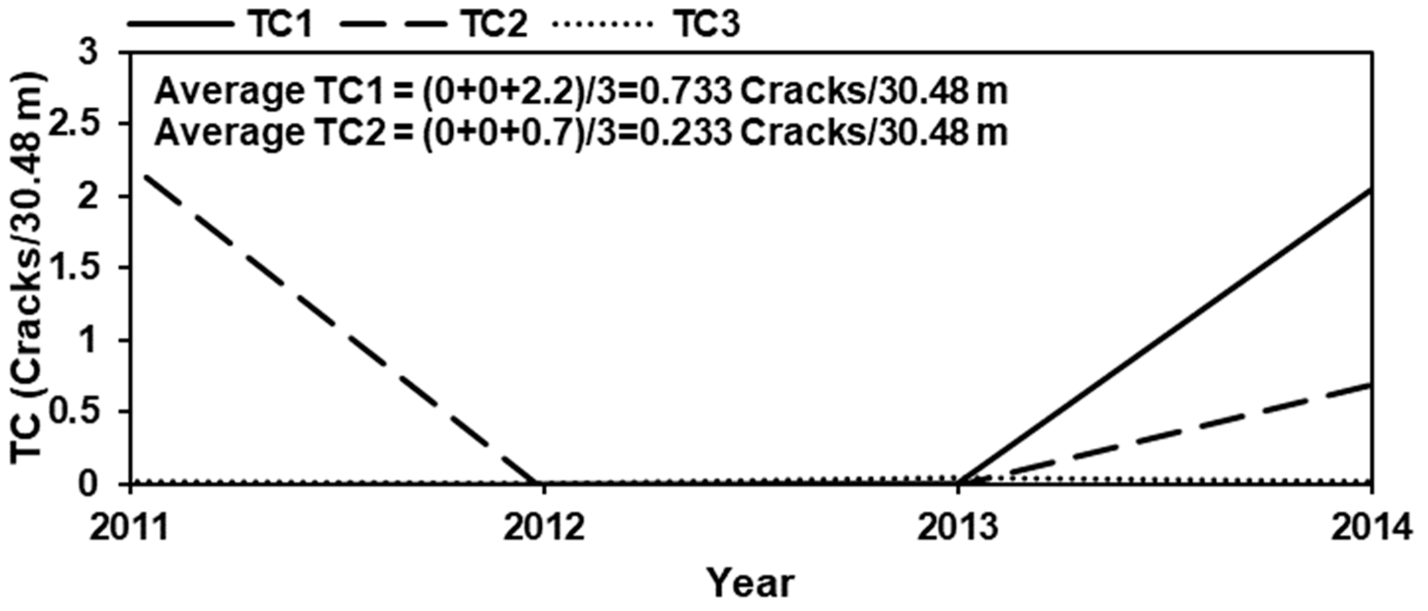
Transverse cracking is expressed as a number of transverse cracks per 30.48 m long pavement segment. It is categorized by codes zero (TC0), one (TC1), two (TC2) and three (TC3). Code zero describes sealed transverse cracks with no roughness. Code one corresponds to the crack width of 6.3 mm or larger with no roughness, and secondary cracking of less than 1.2 m per lane or any width with failed seal (30 cm or more per lane). Code two describes cracks of any width with noticeable roughness that is due to a depression or bump. This includes cracks with more than 1.2 m of secondary cracking without roughness. Code three describes cracks of any width with significant roughness that is due to a depression or bump and with secondary cracking that is more severe than in the case of code two.
Figure 4 shows the evolution of TC1, TC2 and TC3 versus time. The corresponding average rate of change of TC1 since the year of last pavement treatment is 0.733 cracks/30.48 m/year while for TC2 it is 0.233 cracks/30.48 m/year. TC3 remains at zero since the last pavement treatment.
2.2.4. Pavement Roughness
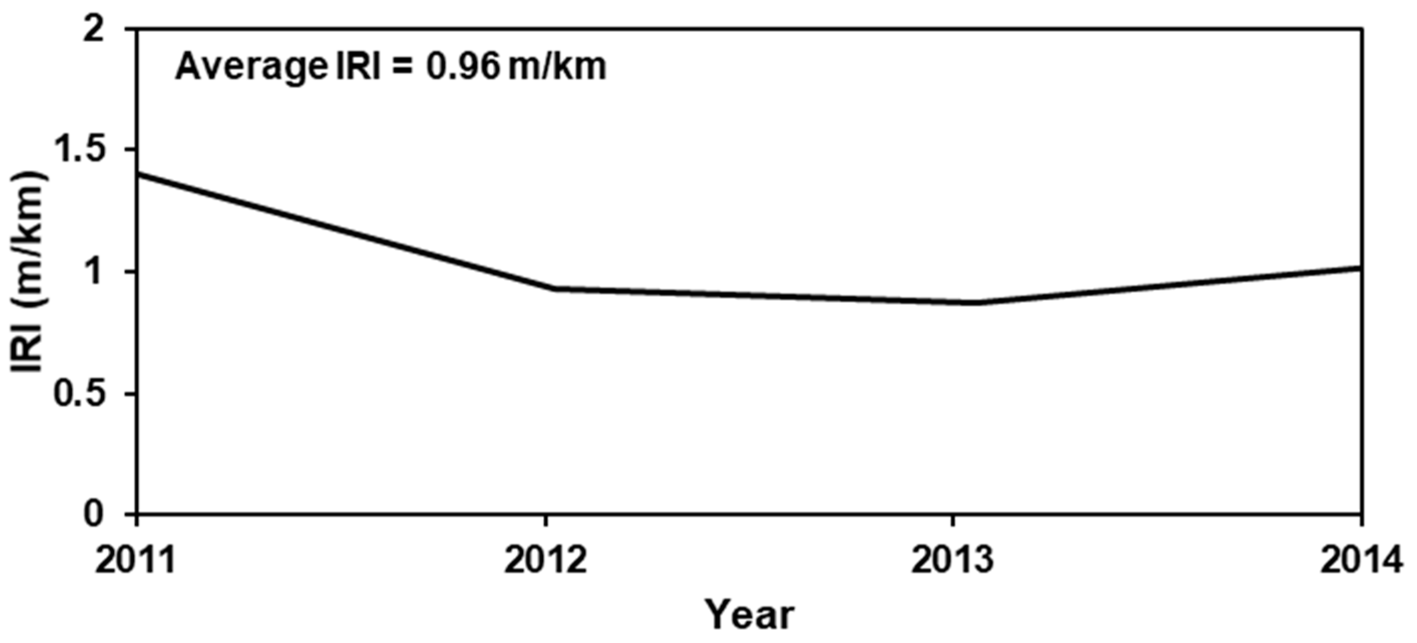
Pavement roughness is expressed in terms of the international roughness index (IRI) whereby the unit used herein is m/km. Code one (1) indicates IRI of less than 1.65 m/km, code two (2) describes IRI that ranges between 1.65 and 2.58 m/km and for IRI larger than 2.58 m/km code three (3) is assigned. The IRI value of less than 1.5 m/km indicates good roughness condition of pavement [
36,
37]. The evolution of IRI for Clay County is depicted in
Figure 5, thus resulting in its average change rate since the last pavement treatment being equal to 0.96 m/km/year.
Cores were extracted from pavement at the time of DCP testing to characterize the pavement condition throughout its depth. The amount of damage was evaluated visually, thus resulting in a percentage of good, fair and poor core that represent the length of core in good, fair and poor condition divided by the total length of the asphalt core. The condition was assessed based on the amounts of cracks and missing material, whether crumbled or not, etc.
2.3. Type of Analyses
Four different statistical analyses were employed in this study including: (1) principal component regression analysis (PCRA), (2) regression analysis (RA), (3) multivariate principal component regression analysis (MPCRA) and (4) multivariate regression analysis (MRA). PCRA is an alternative to regression analysis in the presence of multi-collinearity whereby input variables are highly correlated [
38]. In this study, the strong correlation between
DPI values over depths poses the problem of multi-collinearity. To address this issue, PCRA was employed to investigate the relationship between the changes in rutting code and
DPI values obtained from five depth ranges. RA is a statistical modeling approach for estimating the relationship between an outcome variable and input variables [
39]. RA was used to model the relationship between the average rate of change of rutting severity code and the
DPI value in depth ranging from 0 to 6.35 cm. MPCRA is a multivariate extension of PCRA in case more than one outcome variable is considered in the analysis [
40]. Using MPCRA enabled the estimate of the relationship between the multiple pavement distress indicators (FC1, TC1, TC2, IRI) and the
DPI values for five depth ranges within a single multivariate model rather than fitting separate models for each pavement distress indicator. Similarly, MRA is a multivariate extension of RA [
41]. In this study, MRA was used to incorporate two core variables (good and poor) into a single regression analysis framework.
The statistical analyses identified a number of different significant statistical correlations at a level of 0.05 or smaller. In linear regression analyses, including RA, MRA, PCRA and MPCRA, hypothesis testing can be performed to test statistical significance of the fitted regression model. If the obtained p-value is lower than the α-level (e.g., α = 0.01 or α = 0.05), then the relationship between the outcome and the predictor is statistically significant.
3. Results
Table 2 represents the results, according to which: (1) the
DPI is correlated with the average rate of total rutting, fatigue cracking code one (FC1), and percent of good and poor cores (2) AADTT is correlated with transverse cracking (TC1 and TC2) and (3) the thickness of unbound layer (
Th) is correlated with IRI, and percent of good and poor core.
Significance levels (α),
p-values and adjusted R-squared values for each correlation and the relevant type of statistical analysis are shown in
Table 2. Arrows in
Table 2 indicate the nature of the correlations by showing the trends of dependent variables (increasing ↑, or decreasing ↓) as independent variables in the top row increase (↑).
It is noted that different representations of
DPI values are involved in different
DPI correlations as indicated in the seventh column of
Table 2. The
DPI values obtained at depths of 0 to 6.35 cm, 6.35 to 12.7 cm, 12.7 to 19.05 cm, 19.05 to 25.4 cm and 25.4 to 31.75 cm are denoted by DPI1, DPI2, DPI3, DPI4 and
DPI5, respectively.
Table 3 provides further clarification of
DPI correlations. Two correlations between the total rutting rate and
DPI, which were obtained by PCRA and RA, are shown in
Table 2. The PCRA relates total rutting to the mean values of DPI1, DPI2, DPI3, DPI4 and
DPI5 for each pavement segment. The RA analysis relates the total rutting rate to mean value of DPI1 only for each pavement segment. In addition, MPCRA resulted in fatigue cracking code one (FC1) being correlated with the minimum values of DPI1 through
DPI5 for each pavement segment. Finally, MRA correlates percent of good and poor cores percent with each individual value of
DPI5.
3.1. PCRA Analysis
The correlation between DCP and rutting code change rate from PCRA is given by Equation (2):
where
is average rate of change of rutting severity code (/year) for a given segment since the last treatment,
is mean
DPI value (mm/blow) in depth 0 to 6.3 cm for a given segment,
is mean
DPI value (mm/blow) in depth 6.3 to 12.7 cm for a given segment,
is mean
DPI value (mm/blow) in depth 12.7 to 19.05 cm for a given segment,
is mean
DPI test (mm/blow) in depth 19.05 to 25.4 cm for a given segment and
is mean
DPI value (mm/blow) in depth 25.4 to 31.75 cm for a given segment.
Equation (2) can be interpreted as that rutting rate is positively correlated with mean
DPI values from depths ranging from 0 to 31.75 cm. That is, as mean
DPIs increase the rutting code tends to be higher. As shown in
Table 2, the adjusted R-squared value corresponding to Equation (2) is 0.5473, thus implying that a 54.73% change rate in rutting severity code can be explained by
DPI test results.
The correlation between
DPI and
CBR used by KDOT [
42] is given by Equation (3):
where
CBR is in percent, and
DPI is in mm/blow. Based on Equation (3) the regression model described by Equation (2) can be rewritten as:
where
is mean
CBR value (%) in depth 0 to 6.3 cm for a given segment,
is mean
CBR value (%) in depth 6.3 to 12.7 cm,
is mean
CBR value (%) in depth 12.7 to 19.05 cm,
is mean
CBR value (%) in depth 19.05 to 25.4 cm and
is mean
CBR value (%) in depth 25.4 to 31.75 cm.
Equation (4) can be explained as that rutting average rate is negatively correlated with mean CBR values from depths ranging from 0 to 31.75 cm.
3.2. RA Analysis
Alternatively, based on RA, the change of rate of rutting code can be expressed in terms of average DPI1 value. The corresponding model is given by:
Equation (5) can be described as determining that rutting is positively correlated with
That is to say, rutting code tends to be higher as
increases. Furthermore, the adjusted R-squared value corresponding to Equation (5) is 0.6504, thus implying that 65.04% of rutting can be explained by
. Equation (5) can be modified by using Equation (3), thus obtaining:
Equation (6) indicates that smaller average CBR value from depth of 0 to 6.3 cm results in the larger average change rate of rutting severity code.
3.3. MPCRA Analysis
Four different statistical models resulted from the MPCRA analysis. The first model correlates
DPI values to fatigue cracking code one (FC1) according to:
where
is an average value of fatigue cracking code one (m/30.48 m/year) for a given segment since the last treatment,
DPI1
min is minimum
DPI value (mm/blow) in depth 0 to 6.3 cm for a given segment,
DPI2
min is minimum
DPI value (mm/blow) in depth 6.3 to 12.7 cm,
DPI3
min is minimum
DPI value (mm/blow) in depth 12.7 to 19.05 cm,
DPI4
min is minimum
DPI value (mm/blow) in depth 19.05 to 25.4 cm and
DPI5
min is minimum
DPI value (mm/blow) in depth 25.4 to 31.75 cm.
Equation (7) shows that as the minimum DPI in depths ranging from 0 to 31.75 cm reduces, the fatigue cracking code one tends to increase. The corresponding adjusted R-squared value is 0.2984, thus implying that 29.84% of fatigue cracking code one can be explained by DCP test results. Although this finding seems initially contradictable, it is noted that it was found that DCP test results have a relation only with fatigue cracking code one. Hence, no statistically notable relations were obtained between DPI values and fatigue cracking codes two, three or four. As a result, this finding can be explained as that the initiation of fatigue cracking was found to be negatively correlated to minimum DPI values for a given pavement segment.
Based on Equation (3) the regression model described by Equation (7) can be rewritten as:
where
CBR1
min is minimum
CBR value (%) in depth 0 to 6.3 cm for a given segment,
CBR2
min is minimum
CBR value (%) in depth 6.3 to 12.7 cm,
CBR3
min is minimum
CBR value (%) in depth 12.7 to 19.05 cm,
CBR4
min is minimum
CBR value (%) in depth 19.05 to 25.4 cm and
CBR5
min is minimum
CBR value (%) in depth 25.4 to 31.75 cm.
The second model correlates the truck traffic volume (AADTT) with transverse cracking code one (TC1). The corresponding equation is given by:
where
is the average transverse cracking code one (no. of cracks/30.48 m) for a given segment since the last treatment and
is an average annual daily truck traffic (no. of trucks/day) since the last treatment. Equation (9) shows that as average AADTT increases average transverse cracking code one (TC1) tends to be higher. Furthermore, the adjusted R-squared value for this correlation is 0.1698. Thus, the truck traffic volume can explain the 16.98% of transverse cracking code one.
The third model correlates transverse cracking code two (TC2) with the truck traffic volume. The corresponding equation is given by:
where
is an average transverse cracking code two (no. of cracks/30.48 m) for a given segment since the last treatment. Equation (10) indicates that as the average AADTT increases average transverse cracking code two (TC2) tends to be higher. Moreover, the adjusted R squared value for this correlation is 0.3732. Hence, the 37.32% of transverse cracking code two can be described by truck traffic volume.
Equations (9) and (10) may at first appear counterintuitive. Specifically, transverse cracking is thought to be primarily thermally induced. Nevertheless, no correlation was found between the AADTT and transverse cracking code zero (TC0), and thus no correlation between traffic volume and initiation of transverse cracking. It seems to be reasonable that daily truck traffic may have an influence on the evolution of transverse cracking after it has been thermally initiated. Specifically, the adjusted R-squared for TC2 is almost more than twofold that of TC1.
The fourth model provides the relation between pavement roughness and thickness of unbound layer. The corresponding equation is given by:
where
is an average value of international roughness index (m/km) since the last pavement treatment and
Th is the thickness of unbound layer (mm). The adjusted R-squared value that corresponds to Equation (10) is 0.6279, so the 62.79% of average IRI can be explained by the thickness of unbound layer. Furthermore, as expected average IRI is negatively correlated with the thickness of unbound layer.
3.4. MRA Analysis
A total of 146 DCP tests were carried out for all selected segments.
Table 4 lists the number of DCP tests for each pavement segment used in this analysis.
The first MRA model that resulted from this analysis is described by:
where
GC is an amount of good core (%/100),
DPI5 is an individual
DPI value (mm/blow) in depth 25.4 to 31.75 cm and
Th is the thickness of unbound layer (mm). The corresponding adjusted R-squared value is 0.159, thus showing that the 15.919% of good core can be interpreted by the value of
DPI5 and the thickness of unbound layer.
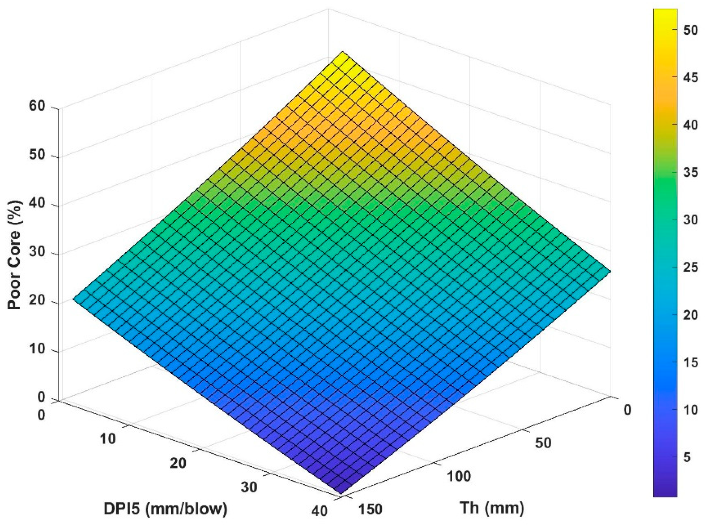
The second MRA model is described by:
where
PC is an amount of poor core (%/100) and
Th is the thickness of unbound layer (mm). The corresponding adjusted R-squared value is 0.1772, so the value of
DPI5 and the thickness of unbound layer can explain the 17.72% of poor core. Equations (12) and (13) imply that as
DPI5 increases or
CBR5 decreases the percentage of good quality core tends to be higher, whereas the percentage of the bad quality core reduces. In addition, as the thickness of unbound layer increases, the percentage of good quality core in the analysis increases, in contrast to the percentage of bad quality core. The effect of the thickness of unbound layer is as expected.
The effect of
DPI5 value on the percent of good and poor core may appear contradictory at first. Nevertheless, it is in accordance with the correlation between the mean values of DPI1 through
DPI5 with fatigue cracking code one (FC1) that was deduced from MPCRA analysis. An increase in a minimum
DPI value within a given pavement segment essentially appears to shift the type of distress from initiation of fatigue cracking to increase in total rutting. Specifically, an increase in minimum
DPI indicates a more uniform subgrade. Consequently, less fatigue cracking likely decreases the amount of poor core, thus increasing the amount of good core. Four additional statistical models were considered in this group for assessing the importance of each predictor in the regression models. The additional models consider only
DPI5 or only the thickness of unbound layer as predictors for the percent of good and poor core. The corresponding values of adjusted R-squared are shown in
Table 5. It is noted that the exclusion of thickness from the models listed in
Table 5 results in a larger decrease in adjusted R-squared than the exclusion of
DPI5. This implies that DPI has a weaker influence on core analysis than the thickness of unbound layer.
3.5. Applications and Implementations
3.5.1. Rutting
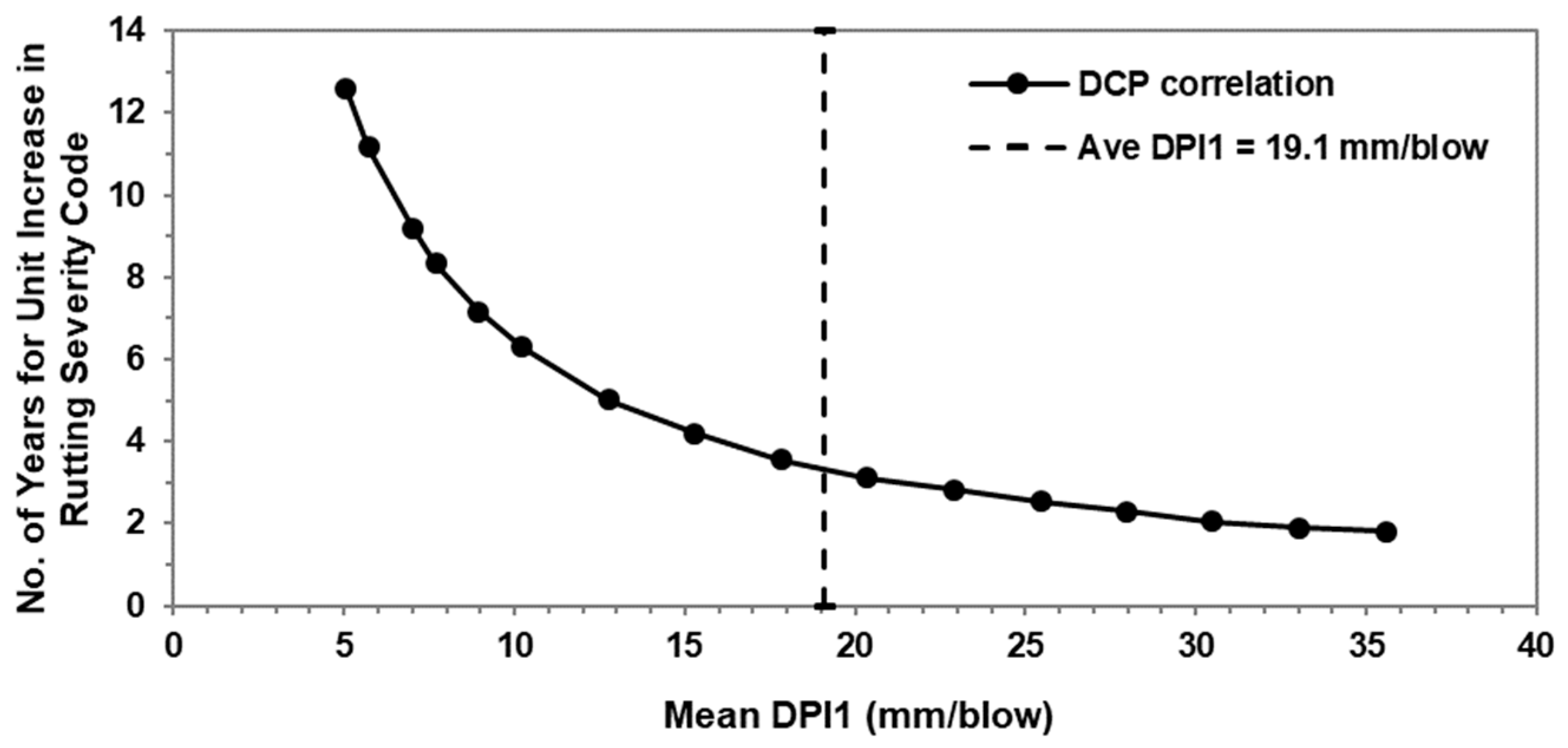
The regression model given by Equation (5) provides mean rate of change of the rutting severity code in terms of the mean DPI1 value, from which the time interval for unit increment in rutting severity code can be expressed as:
where
is a time interval (yr) that corresponds to the unit increase in rutting code since the last treatment. A graphical representation of Equation (12) is shown in
Figure 6. To determine an acceptable
value within the top 6.35 cm of a subgrade soil both Equation (14) and
Figure 6 can be utilized.
It is noted that the average DPI1 value for all pavement segments considered in this study is 19.1 mm/blow. Furthermore, it is predicted by the RA model that it takes 3.34 years for the unit increase in the rutting severity code at mean DPI1 value of 19.1 mm/blow.
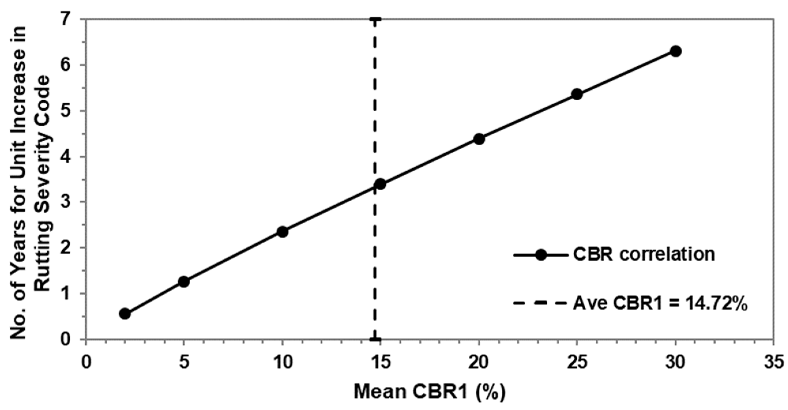
Equation (14) can be further modified by combining it with Equations (3) and (14), thus resulting in:
Equation (15) is depicted in
Figure 7. The average
CBR value of 14.72% within the top 6.35 cm m was obtained for the pavement sections considered in this study. In summary, Equations (14) and (15) along with
Figure 6 and
Figure 7 are useful for selecting the acceptable average value of CBR1. Thus, the acceptable value depends on the acceptable rate of rut deterioration and reasonable amount of subgrade compactness.
3.5.2. Core Quality
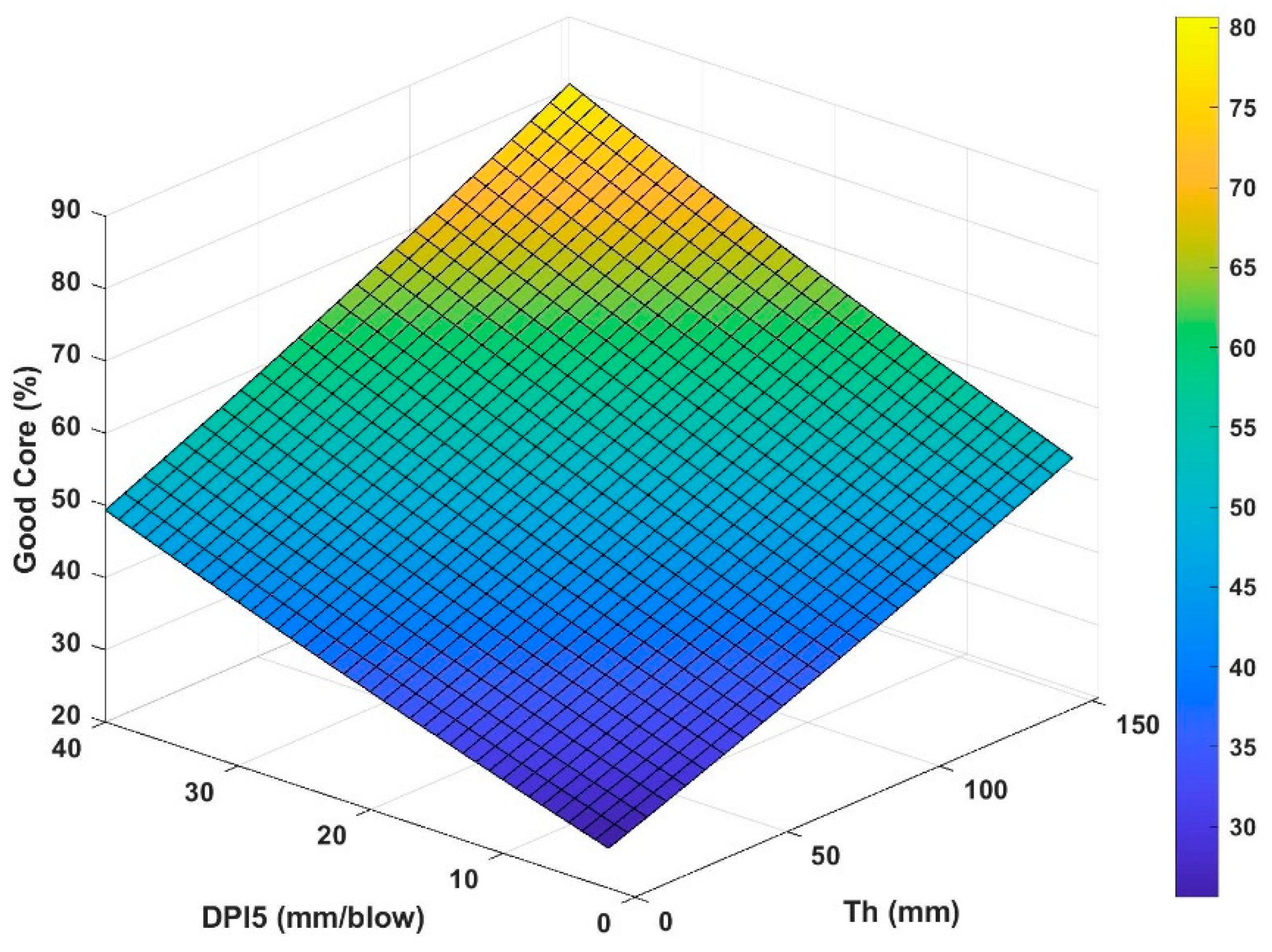
In this section, the percent of good, poor, and fair cores is expressed in terms of the thickness of unbound layer and
DPI5 according to the results of MRA analysis.
Figure 8 is the graphical form of Equation (12) and it can be helpful for deciding about acceptable values of
DPI5.
Percent of poor core for different thicknesses of unbound layer can be obtained from Equation (13), which is depicted graphically in
Figure 9.
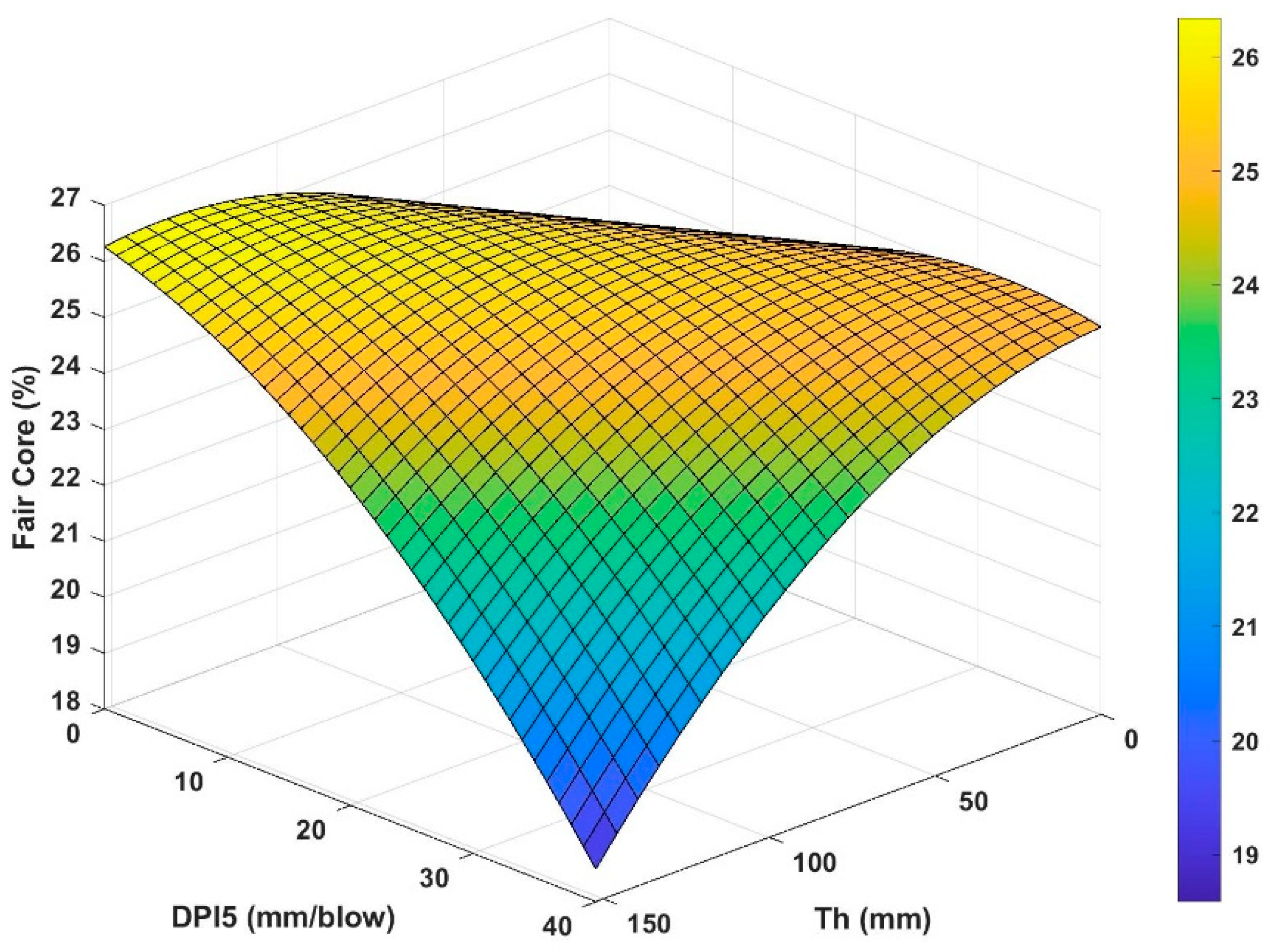
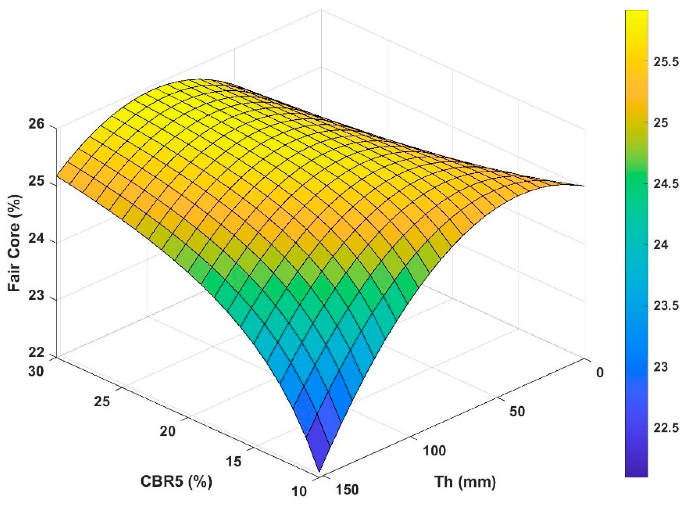
The percent of core in fair condition can simply be calculated by subtracting the sum of the percentages of good and poor cores from 100%. The corresponding graph is depicted in
Figure 10.
Figure 8,
Figure 9 and
Figure 10 show increase in percent of good core and decrease of poor core with increased thickness of unbound layer, as expected. Nevertheless, an increase in DPI causes increased amount of good core and decreased amount of poor core. This may be surprising. Nevertheless, this particular DPI was measured at depths ranging from 25 cm to 31.75 cm below the bottom of the asphalt core while those DPIs measured at shallower depths did not exhibit statistically significant correlation with the quality of core. The trend of fair core is simply the outcome of the trends of good and poor cores.
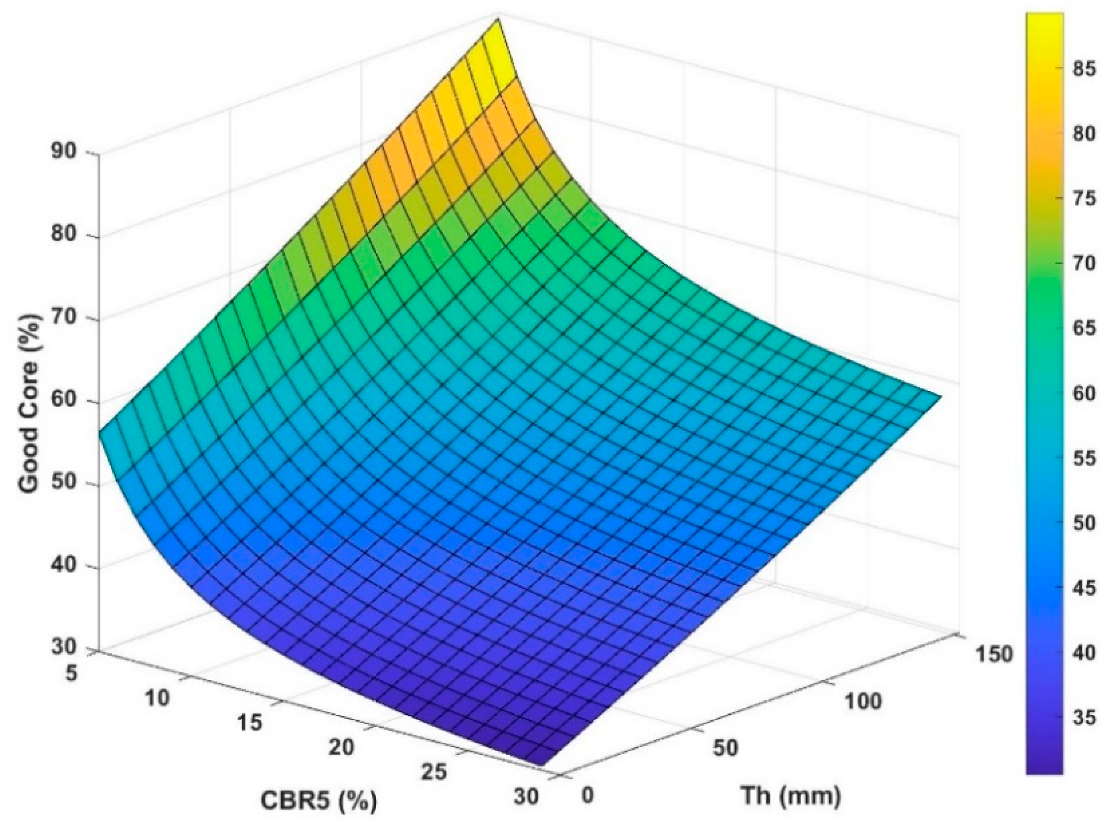
Combining Equation (3) with Equation (12) results in:
where
GC (%) is the percent of good core.
Figure 11 presents Equation (16) in a graphical form that can be useful when determining the acceptable
CBR5 value.
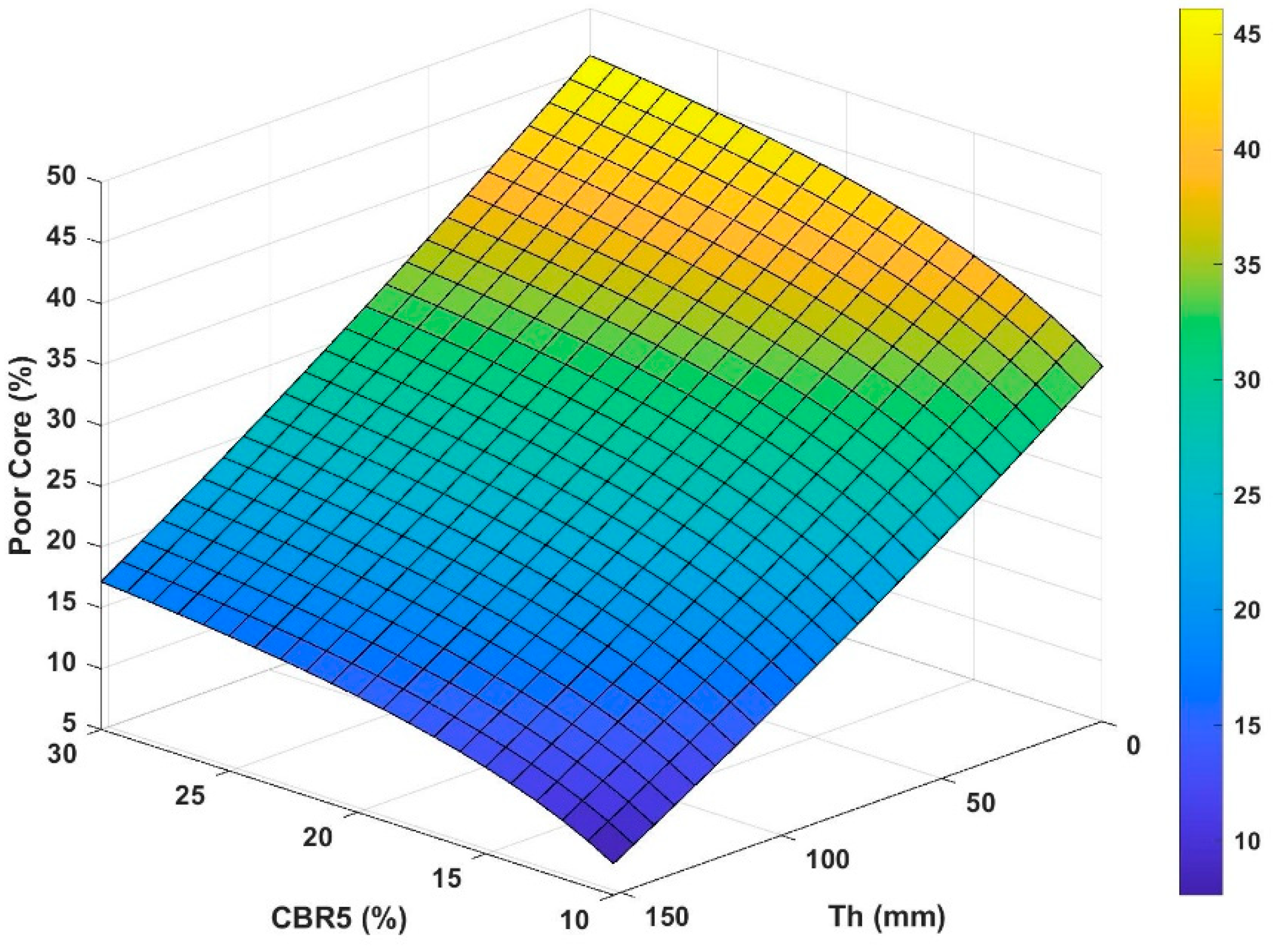
Similarly, Equation (13) can be modified by using Equation (3). The resulting equation is given by:
where
PC is percent of poor core. Equation (17) is depicted in
Figure 12.
Finally, as explained previously the percent of core in fair condition can be determined by subtracting the sum of the percentages of good and poor cores from 100%. The corresponding graph is shown in
Figure 13.
Figure 11,
Figure 12 and
Figure 13 can be useful for determining the acceptable
CBR value. According to these figures the largest magnitude of change in the percent of good, poor and fair cores occurs for
CBR5 smaller than 10%. The changes in the percent of good and poor cores for
CBR5 values between 10% and 15% are about the same as are the changes between
CBR5 values between 15% and 30%. Thus, the rate of change of the percent of good and poor cores reduces slowly as
CBR5 increases.
5. Conclusions
Multiple statistical analyses were conducted to develop pavement performance prediction models for flexible pavements in the state of Kansas, with emphasis on the effects of subgrade and unbound layers. To this end, the input variables included results of DCP tests within the top 0.32 m of subgrade, thickness of unbound layer and traffic volume (AADTT). The output variables were pavement distresses including: (1) rutting, (2) fatigue cracking, (3) thermal cracking, (4) pavement roughness and (5) asphalt core condition.
It was found that the statistically significant correlations that reflect the effects of subgrade are: (1) correlations between DCP or CBR tests and the rate of change of the of total rutting code, fatigue cracking code one and percent of good and poor cores. These correlations indicate that increase in mean DPI values for a given pavement segment; thus, a decrease in the corresponding mean CBR values accelerates total rutting. Furthermore, an increase in minimum DPI values for a given pavement segment results in a decrease in fatigue cracking code one. Finally, an increase in individual DPI values at depths ranging from 25.4 cm to 31.75 cm increases the corresponding amount of good core while decreasing the amount of poor core. In summary, improved compactness and strength of subgrade that is reflected in decreasing DPI values decreases the rate of rutting, while more uniform compactness of subgrade decreases the amount of fatigue cracking. Furthermore, the correlation between CBR within the top 6.35 cm of subgrade with the rate of change of rutting code enabled development of a recommendation for the selection of a minimum acceptable value of CBR depending on the acceptable time required for unit increase in the rutting code.
Another statistically significant correlation reflecting the effect of unbound layer on the accumulation of pavement distress indicates that the increased thickness of unbound layer decreases the average pavement roughness (IRI). Finally, statistically significant positive correlation was found between the average value of AADTT and amount of transverse cracking codes one and two. Consequently, the increased amount of traffic increases propagation of transverse cracks but not their initiation.
In summary, the pavement performance prediction models developed in this study achieved the goals of characterizing and quantification the effects of subgrade and unbound layers on accumulation of pavement distresses, and development of scientifically based recommendation for selection of the minimum acceptable CBR value.
Finally, the statistical approach used in this study may contribute toward analysis of pavement historical distress data. Nevertheless, as mentioned previously, use of distress indicator codes is not the most appropriate in conjunction with pavement performance prediction research. Thus, the important recommendation for the related future research is to use more detailed measurements of pavement distress such as the actual amount of rutting, area of cracked pavement, etc.


 ,
, 


