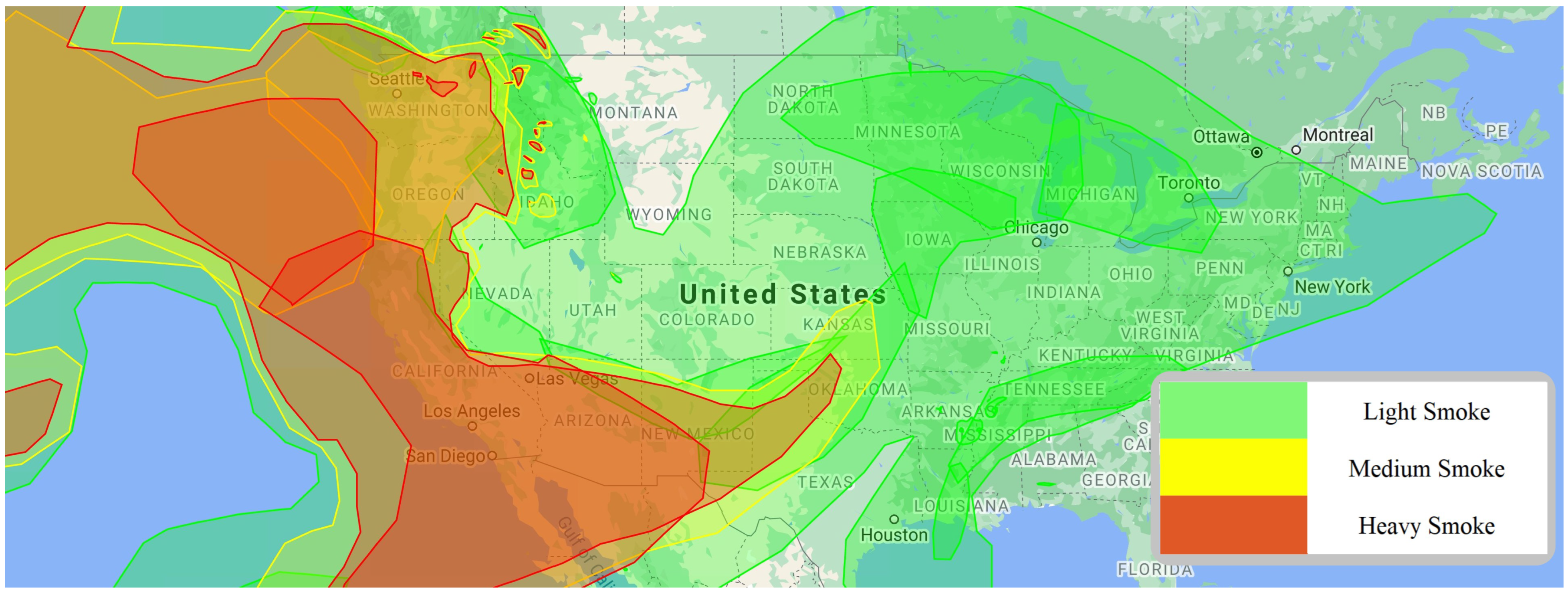
Figure 1.
The span of smoke from wildfires on 9 September 2020. Smoke layers are from the NOAA HMS [
17]. Map data from Google [
18].
Figure 1.
The span of smoke from wildfires on 9 September 2020. Smoke layers are from the NOAA HMS [
17]. Map data from Google [
18].
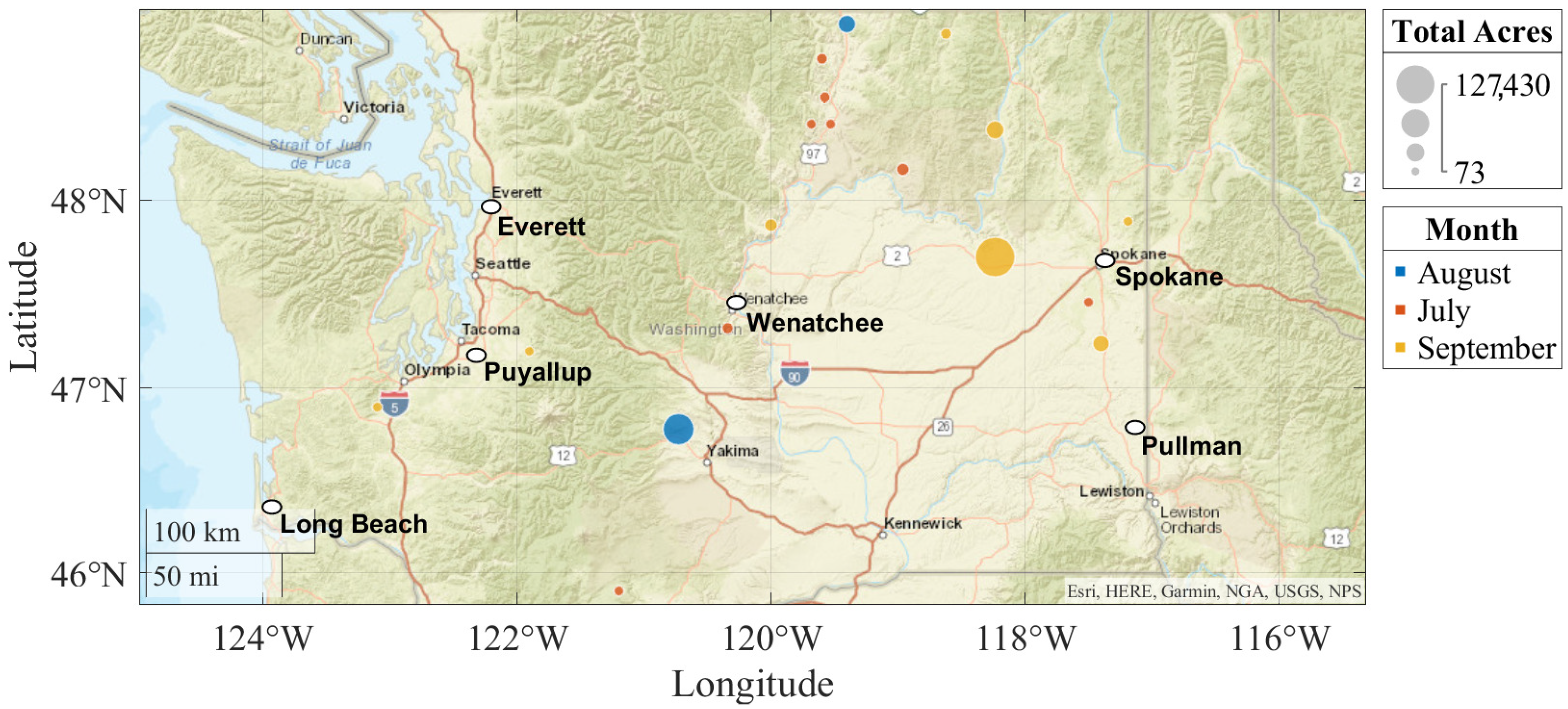
Figure 2.
Geographical localization of all the analyzed cities in this work, and total acres burned due to large fires in the state of Washington, during the months of July, August, and September.
Figure 2.
Geographical localization of all the analyzed cities in this work, and total acres burned due to large fires in the state of Washington, during the months of July, August, and September.
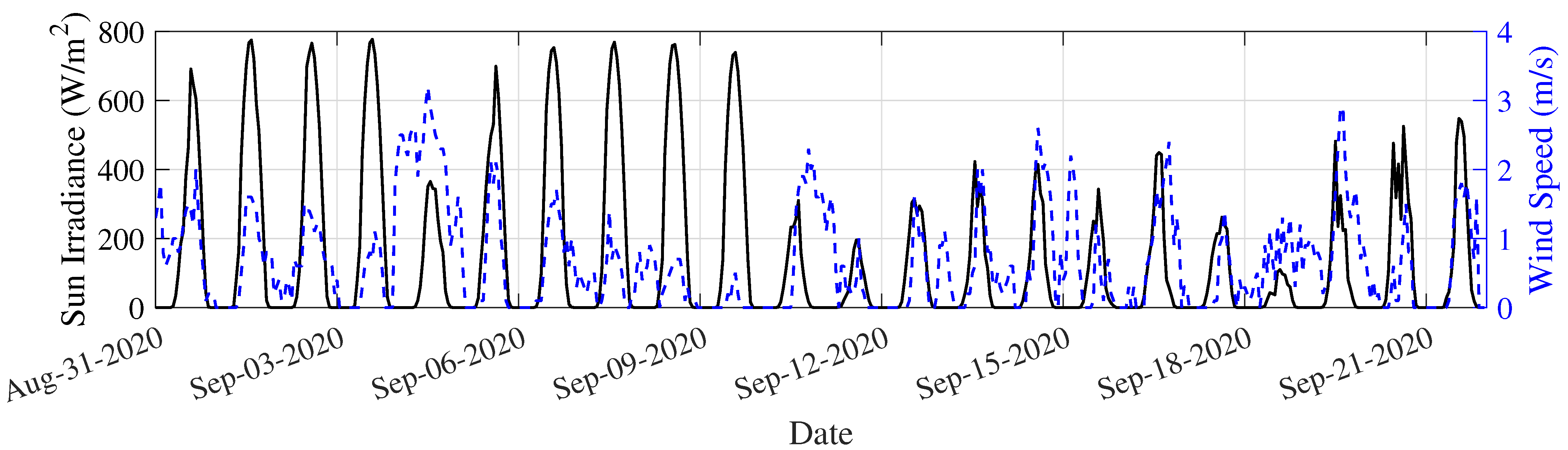
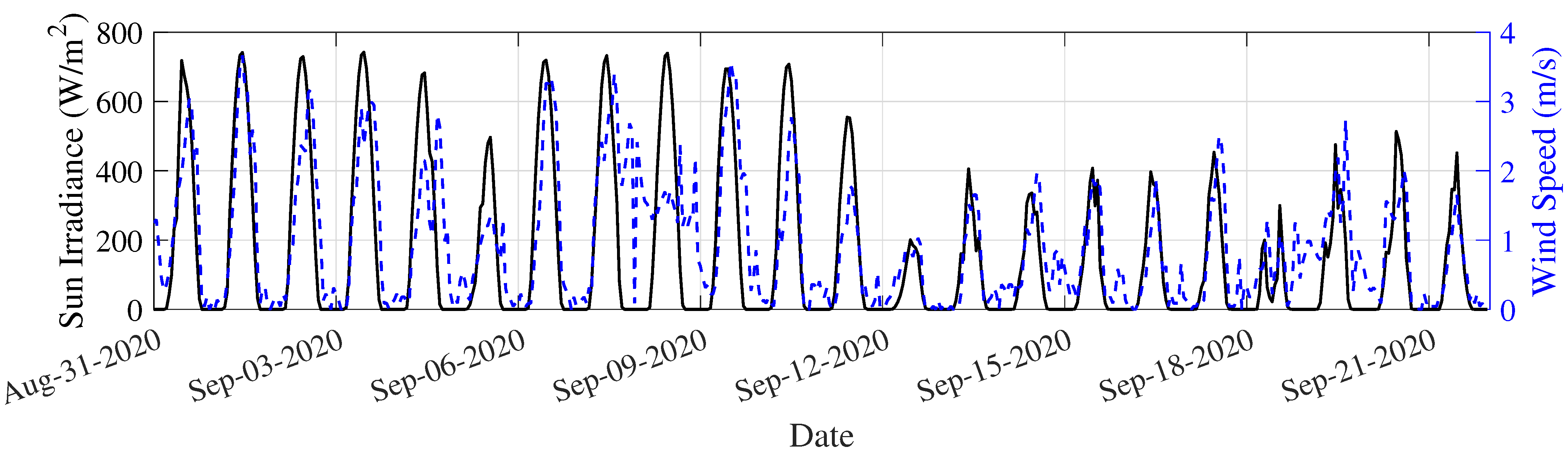
Figure 3.
Solar irradiance (W/m2) and wind speed (m/s) during the first three weeks of September of 2020, in Everett, WA.
Figure 3.
Solar irradiance (W/m2) and wind speed (m/s) during the first three weeks of September of 2020, in Everett, WA.
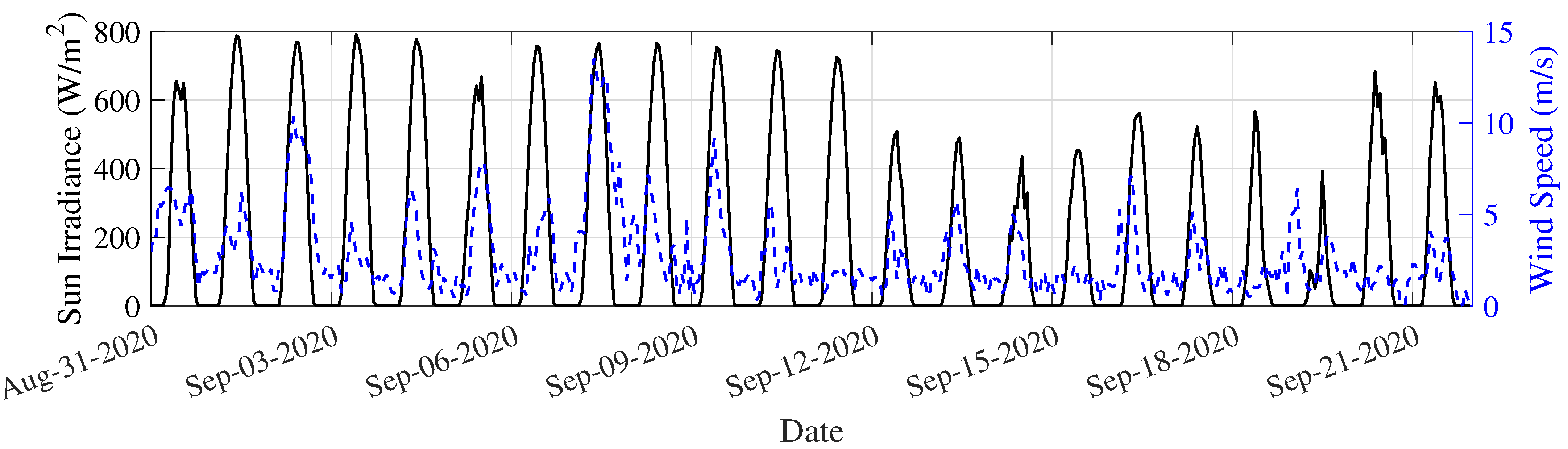
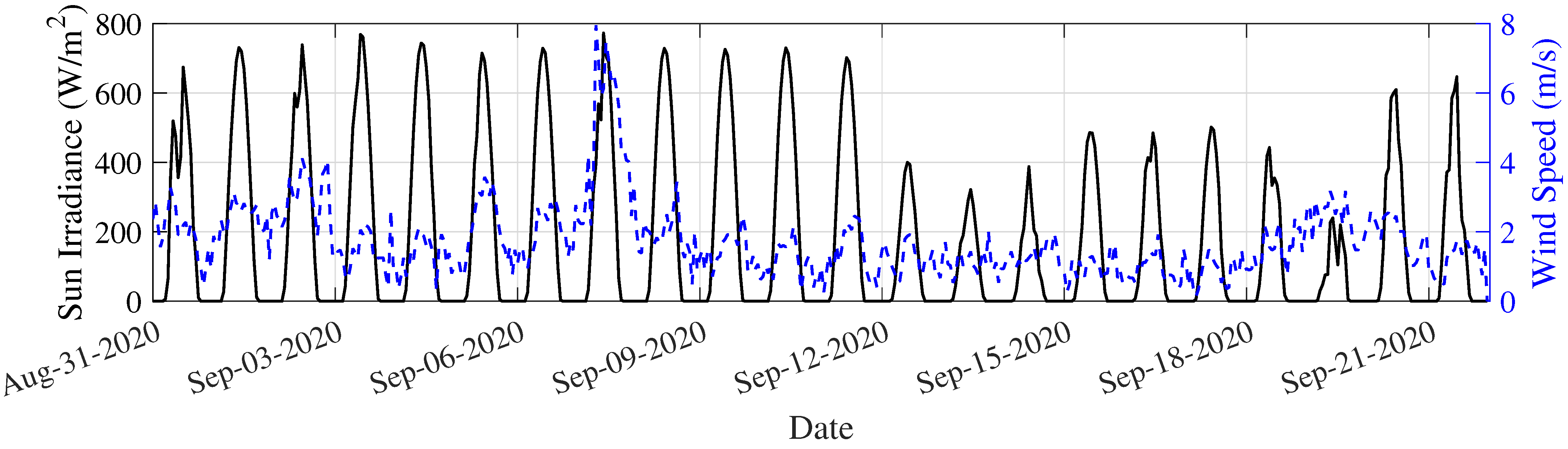
Figure 4.
Solar irradiance (W/m2) and wind speed (m/s) during the first three weeks of September of 2020, in Long Beach, WA.
Figure 4.
Solar irradiance (W/m2) and wind speed (m/s) during the first three weeks of September of 2020, in Long Beach, WA.
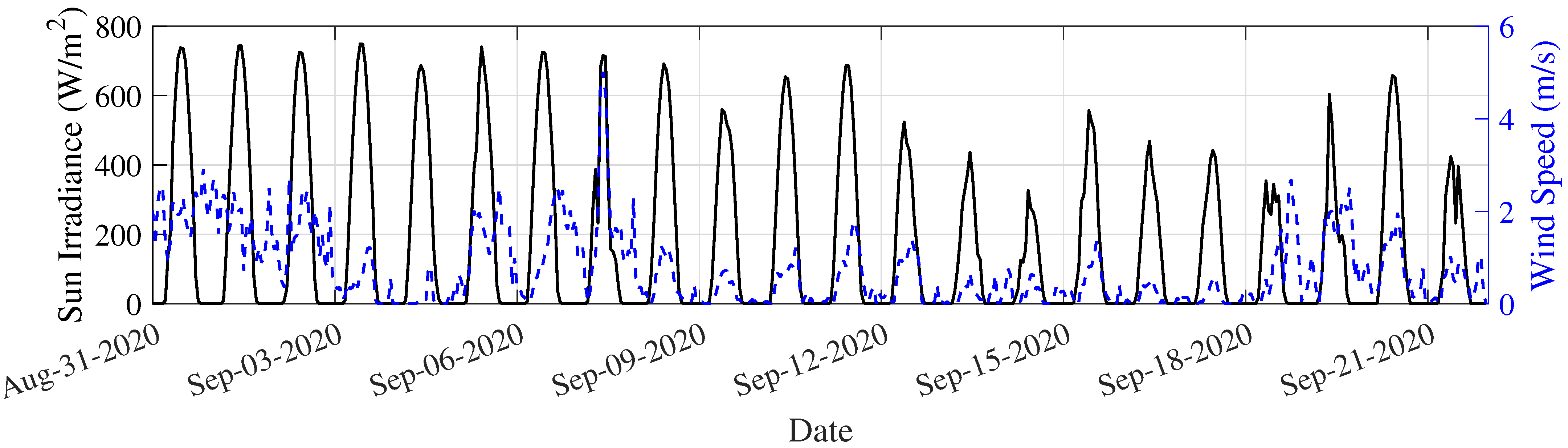
Figure 5.
Solar irradiance (W/m2) and wind speed (m/s) during the first three weeks of September of 2020, in Pullman, WA.
Figure 5.
Solar irradiance (W/m2) and wind speed (m/s) during the first three weeks of September of 2020, in Pullman, WA.
Figure 6.
Solar irradiance (W/m2) and wind speed (m/s) during the first three weeks of September of 2020, in Puyallup, WA.
Figure 6.
Solar irradiance (W/m2) and wind speed (m/s) during the first three weeks of September of 2020, in Puyallup, WA.
Figure 7.
Solar irradiance (W/m2) and wind speed (m/s) during the first three weeks of September of 2020, in Spokane, WA.
Figure 7.
Solar irradiance (W/m2) and wind speed (m/s) during the first three weeks of September of 2020, in Spokane, WA.
Figure 8.
Solar irradiance (W/m2) and wind speed (m/s) during the first three weeks of September of 2020, in Wenatchee, WA.
Figure 8.
Solar irradiance (W/m2) and wind speed (m/s) during the first three weeks of September of 2020, in Wenatchee, WA.
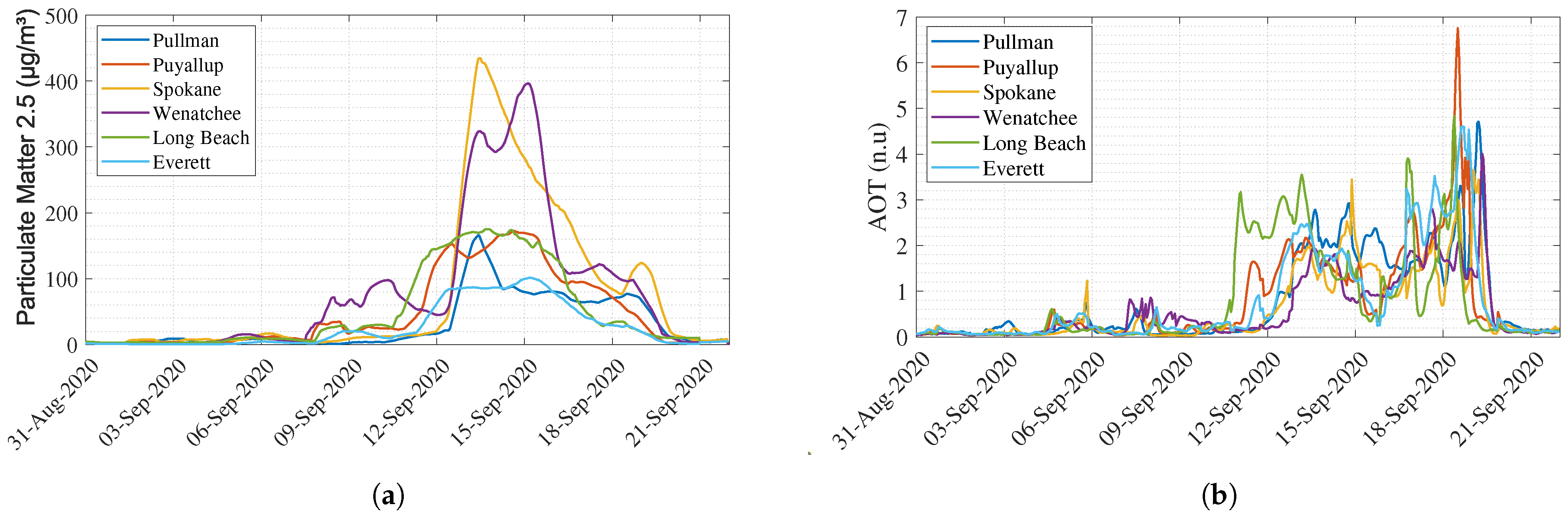
Figure 9.
(a) PM 2.5 and (b) AOT values for the locations analyzed, during the first three weeks of September 2020.
Figure 9.
(a) PM 2.5 and (b) AOT values for the locations analyzed, during the first three weeks of September 2020.
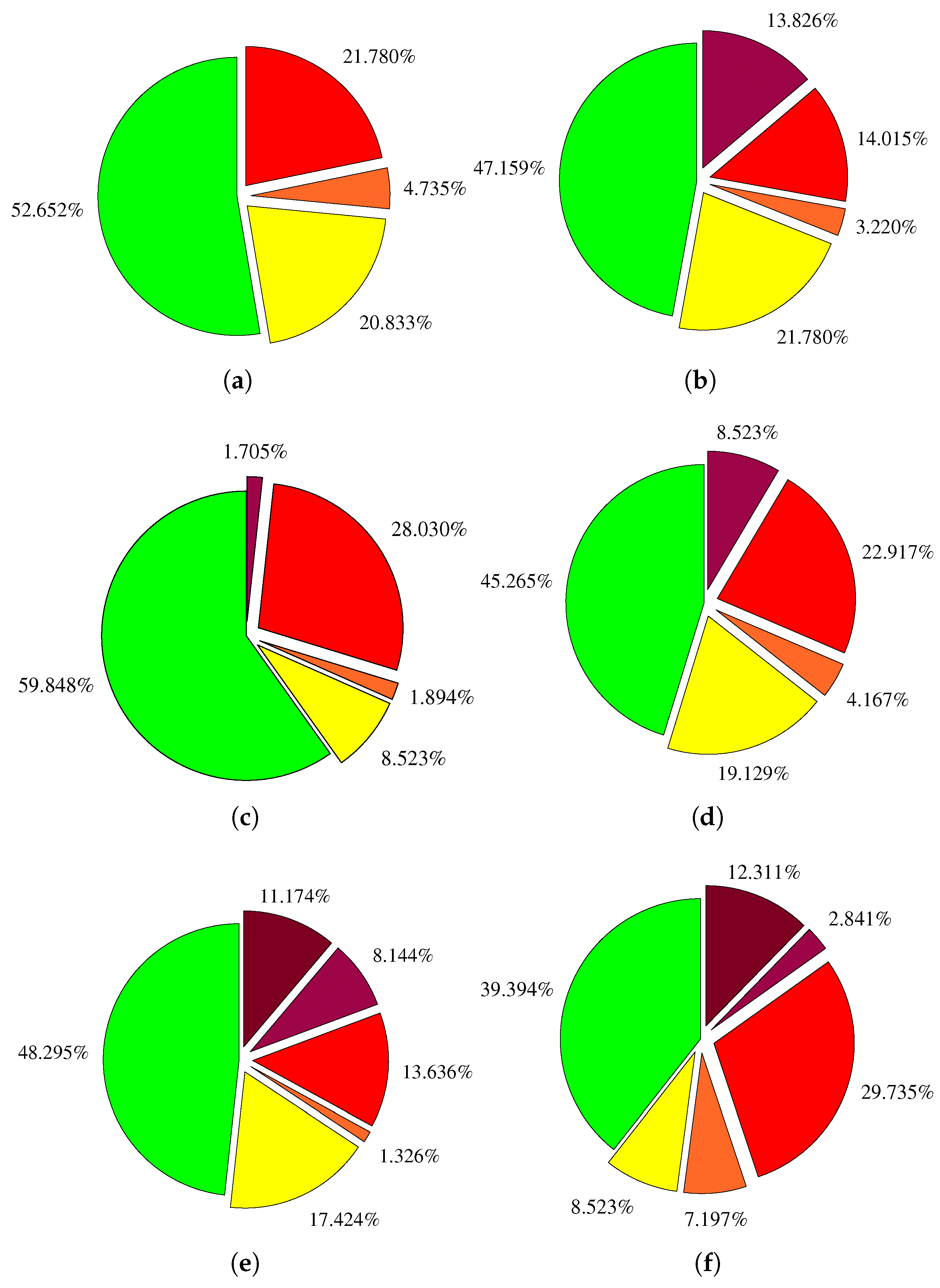
Figure 10.
PM 2.5 level distribution during the first three weeks of September 2020 for the cities of (a) Everett, (b) Long Beach, (c) Pullman, (d) Puyallup, (e) Spokane, and (f) Wenatchee.
Figure 10.
PM 2.5 level distribution during the first three weeks of September 2020 for the cities of (a) Everett, (b) Long Beach, (c) Pullman, (d) Puyallup, (e) Spokane, and (f) Wenatchee.
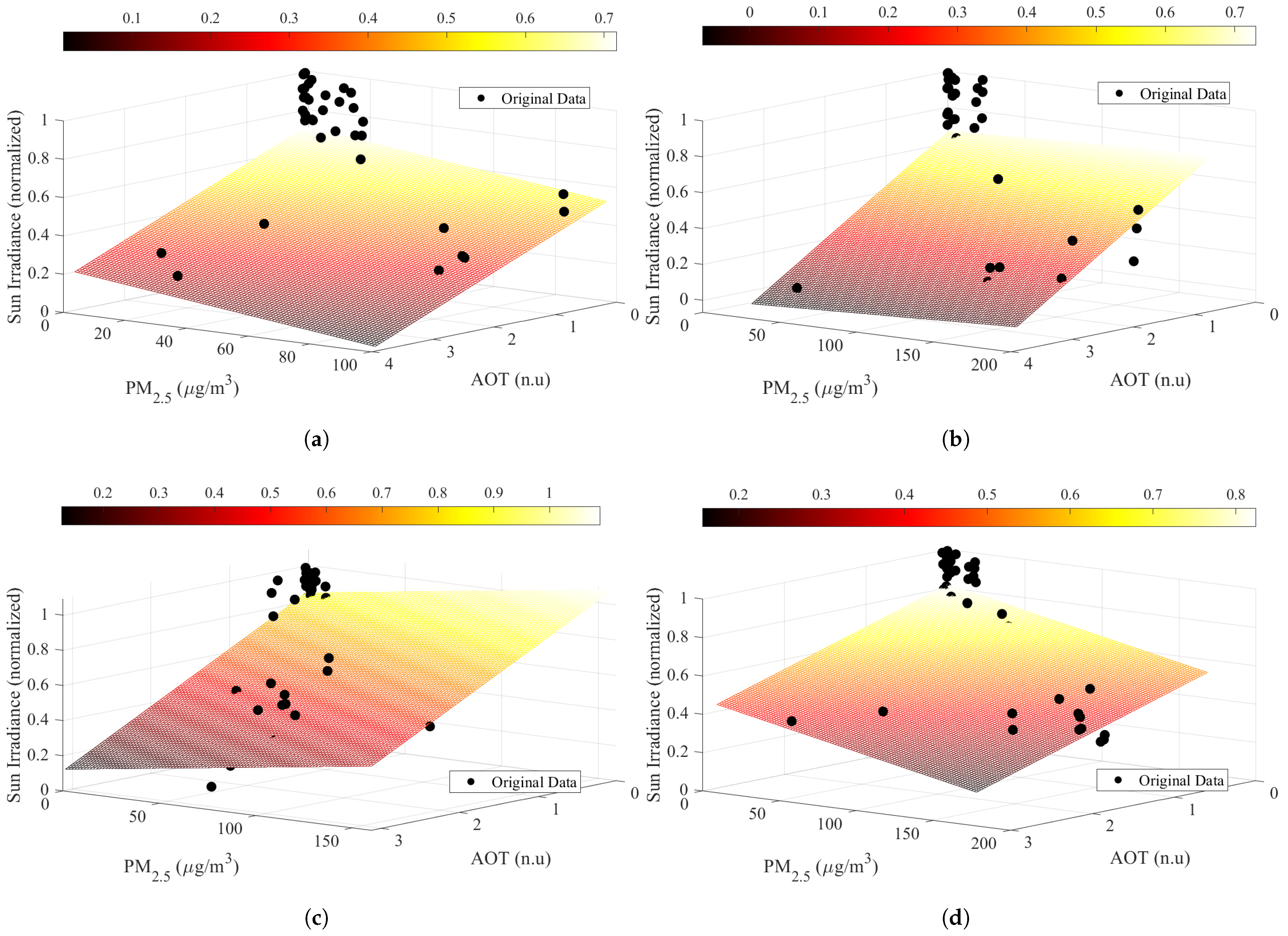
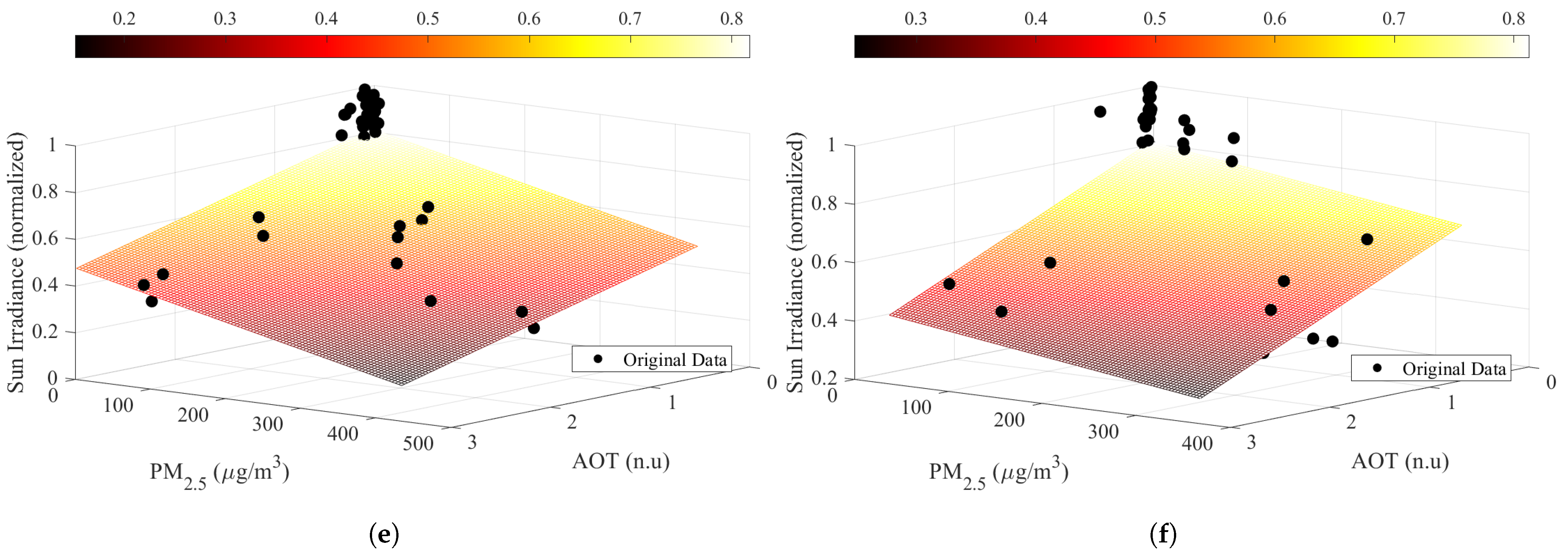
Figure 11.
Multiple linear regression analysis between the solar irradiance, the AOT, and the PM 2.5 data during the 2020 wildfire season for the cities of (a) Everett, (b) Long Beach, (c) Pullman, (d) Puyallup, (e) Spokane, and (f) Wenatchee.
Figure 11.
Multiple linear regression analysis between the solar irradiance, the AOT, and the PM 2.5 data during the 2020 wildfire season for the cities of (a) Everett, (b) Long Beach, (c) Pullman, (d) Puyallup, (e) Spokane, and (f) Wenatchee.
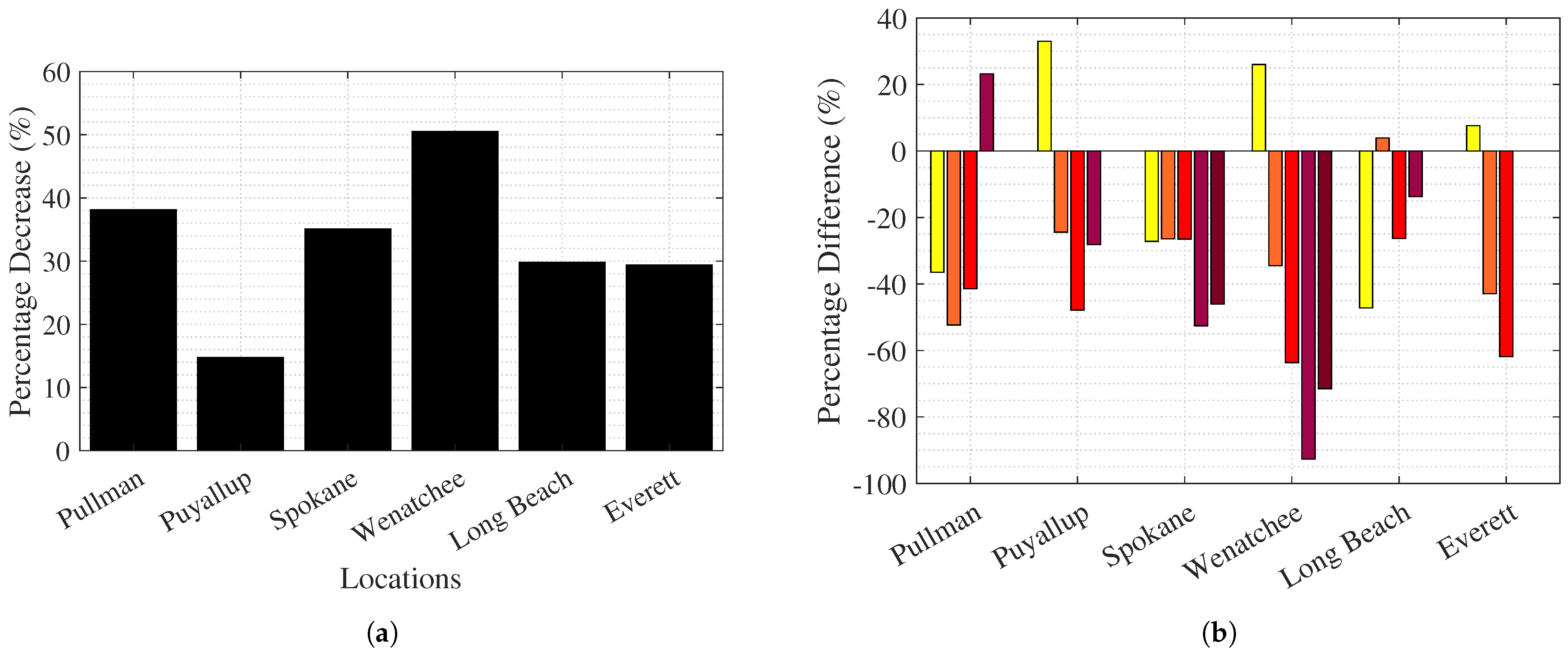
Figure 12.
(a) Wind speed average percentage decrease for the analyzed locations, comparing periods below and above the good PM 2.5 AQI breakpoint, and the (b) wind speed average percentage difference for the analyzed locations, comparing all PM 2.5 AQI breakpoints with normal condition.
Figure 12.
(a) Wind speed average percentage decrease for the analyzed locations, comparing periods below and above the good PM 2.5 AQI breakpoint, and the (b) wind speed average percentage difference for the analyzed locations, comparing all PM 2.5 AQI breakpoints with normal condition.
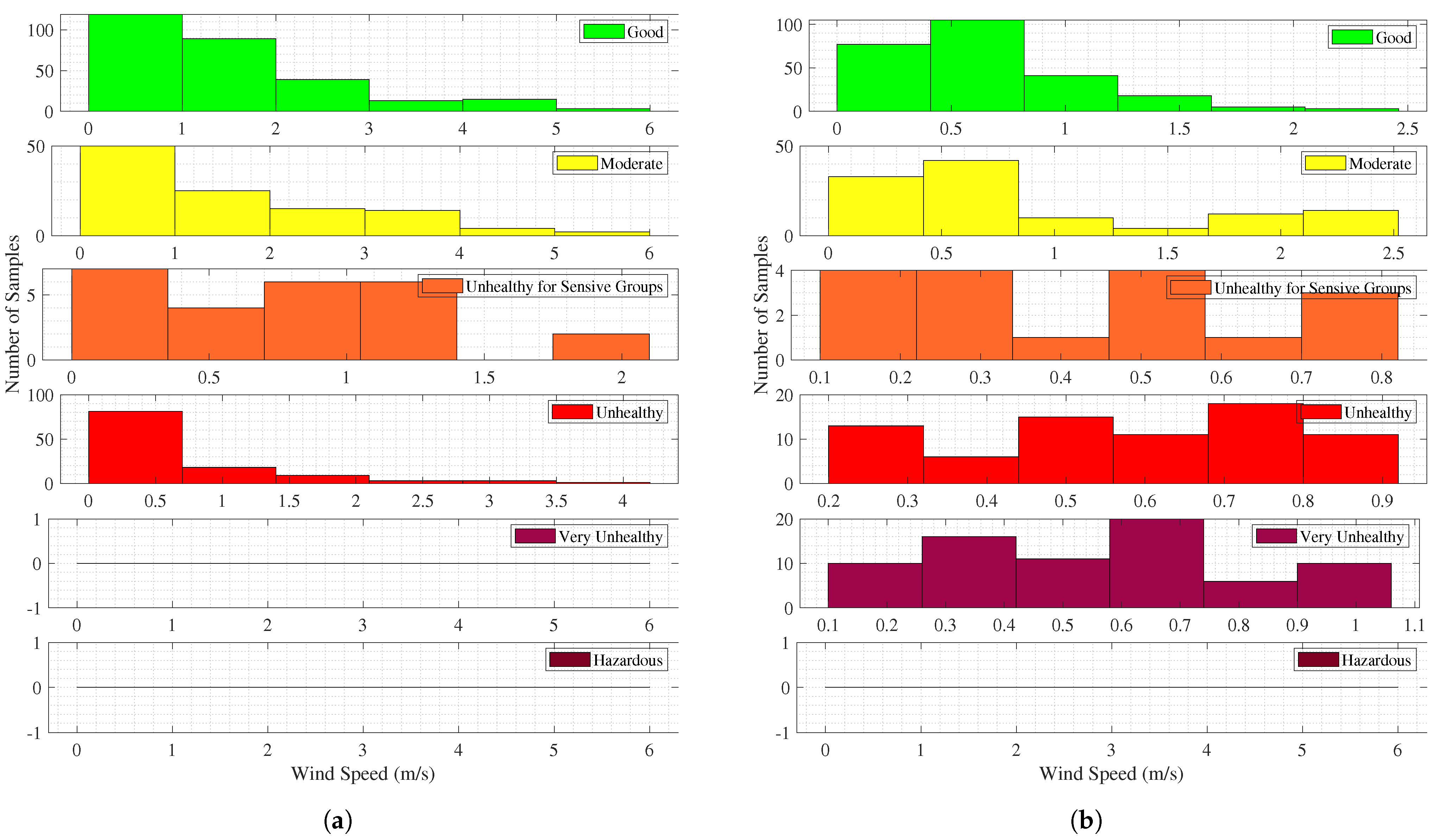
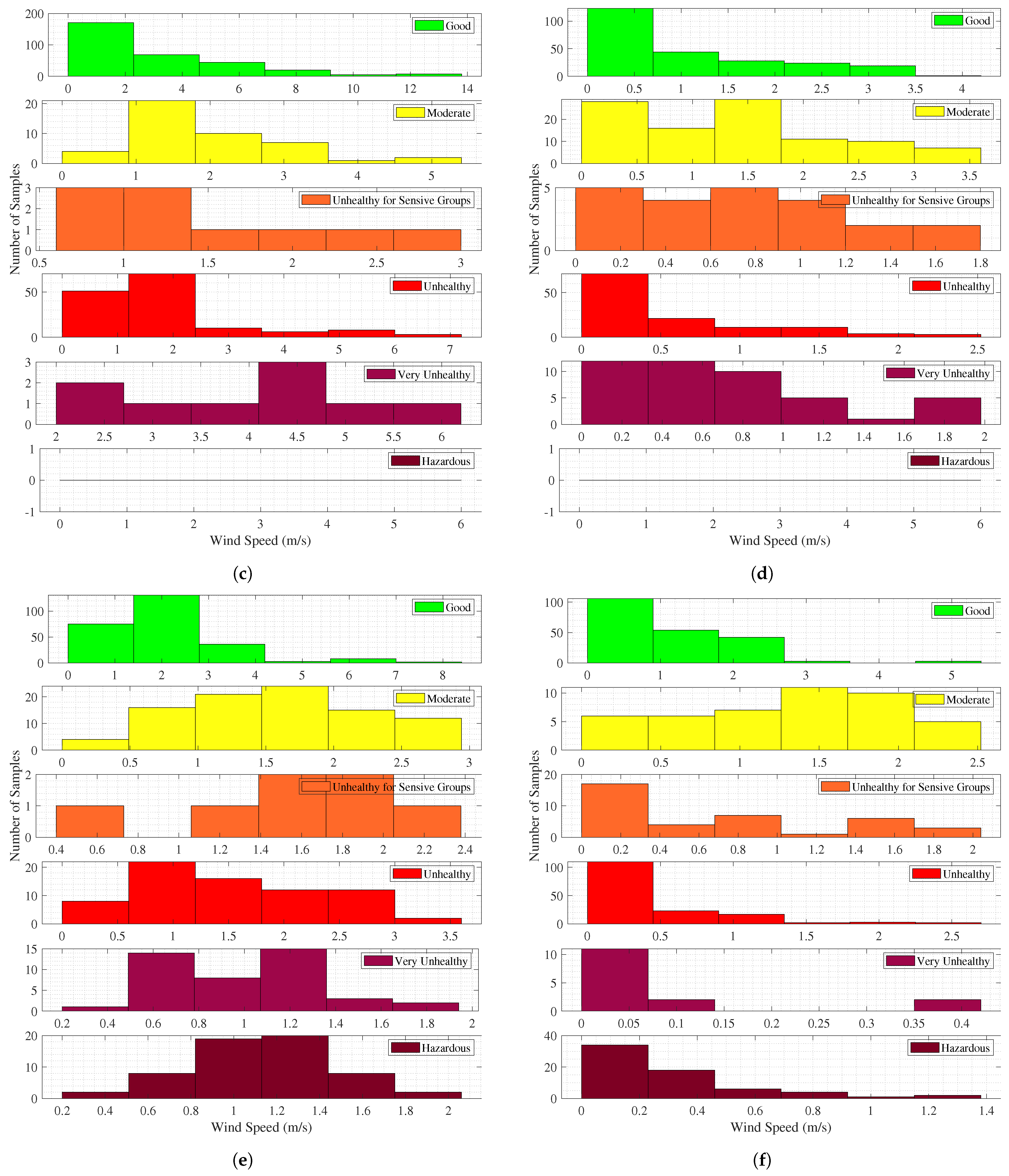
Figure 13.
Wind speed histograms for the cities of (a) Everett, (b) Long Beach, (c) Pullman, (d) Puyallup, (e) Spokane, and (f) Wenatchee, divided by the PM 2.5 AQI categories.
Figure 13.
Wind speed histograms for the cities of (a) Everett, (b) Long Beach, (c) Pullman, (d) Puyallup, (e) Spokane, and (f) Wenatchee, divided by the PM 2.5 AQI categories.
Table 1.
AQI breakpoints, revised in 2012 by the EPA. Table adapted from [
30].
Table 1.
AQI breakpoints, revised in 2012 by the EPA. Table adapted from [
30].
| PM 2.5 AQI Category | PM 2.5 Levels (μg/m3) | Color |
|---|
| Good | 0.0–12.0 | |
| Moderate | 12.1–35.4 | |
| Unhealthy for Sensitive Groups | 35.5–55.4 | |
| Unhealthy | 55.5–150.4 | |
| Very Unhealthy | 150.5–250.4 | |
| Hazardous | ≥250.5 | |
Table 3.
ANOVA analysis for regression for the city of Everett, WA.
Table 3.
ANOVA analysis for regression for the city of Everett, WA.
| | df | SS | MS | F | Fcrit |
|---|
| Regression | 2 | 1.7886 | 0.8943 | 18.5516 | 0.9513 |
| Residual | 60 | 2.8924 | 0.0482 | | |
| Total | 62 | 4.6810 | | | |
Table 4.
ANOVA analysis for regression for the city of Long Beach, WA.
Table 4.
ANOVA analysis for regression for the city of Long Beach, WA.
| | df | SS | MS | F | Fcrit |
|---|
| Regression | 2 | 2.0623 | 1.0311 | 21.3452 | 0.9513 |
| Residual | 56 | 2.7052 | 0.0483 | | |
| Total | 58 | 4.7675 | | | |
Table 5.
ANOVA analysis for regression for the city of Pullman, WA.
Table 5.
ANOVA analysis for regression for the city of Pullman, WA.
| | df | SS | MS | F | Fcrit |
|---|
| Regression | 2 | 1.8183 | 0.9092 | 75.9726 | 0.9513 |
| Residual | 56 | 0.6701 | 0.0120 | | |
| Total | 58 | 2.4885 | | | |
Table 6.
ANOVA analysis for regression for the city of Puyallup, WA.
Table 6.
ANOVA analysis for regression for the city of Puyallup, WA.
| | df | SS | MS | F | Fcrit |
|---|
| Regression | 2 | 1.9639 | 0.9820 | 43.1779 | 0.9513 |
| Residual | 58 | 1.3190 | 0.0227 | | |
| Total | 60 | 3.2829 | | | |
Table 7.
ANOVA analysis for regression for the city of Spokane, WA.
Table 7.
ANOVA analysis for regression for the city of Spokane, WA.
| | df | SS | MS | F | Fcrit |
|---|
| Regression | 2 | 1.6905 | 0.8453 | 50.6302 | 0.9513 |
| Residual | 58 | 0.9683 | 0.0167 | | |
| Total | 60 | 2.6588 | | | |
Table 8.
ANOVA analysis for regression for the city of Wenatchee, WA.
Table 8.
ANOVA analysis for regression for the city of Wenatchee, WA.
| | df | SS | MS | F | Fcrit |
|---|
| Regression | 2 | 1.3400 | 0.6700 | 29.7382 | 0.9513 |
| Residual | 57 | 1.2842 | 0.0225 | | |
| Total | 59 | 2.6241 | | | |
Table 9.
MAE and MSE values for the sun irradiance multiple regression linear model for the analyzed cities.
Table 9.
MAE and MSE values for the sun irradiance multiple regression linear model for the analyzed cities.
| City | Everett | Long Beach | Pullman | Puyallup | Spokane | Wenatchee |
|---|
| MAE (%) | 18.24 | 18.19 | 8.91 | 12.13 | 10.25 | 12.05 |
| r2 | 0.38 | 0.43 | 0.73 | 0.59 | 0.63 | 0.51 |
Table 10.
Wind speeds (m/s) for all the analyzed locations, during different air quality conditions.
Table 10.
Wind speeds (m/s) for all the analyzed locations, during different air quality conditions.
| City | Everett | Long Beach | Pullman | Puyallup | Spokane | Wenatchee |
|---|
| | 1.465 | 0.792 | 3.189 | 1.003 | 2.100 | 1.056 |
| | 1.577 | 0.418 | 2.027 | 1.334 | 1.529 | 1.331 |
| | 0.836 | 0.823 | 1.520 | 0.758 | 1.545 | 0.692 |
| | 0.559 | 0.584 | 1.868 | 0.523 | 1.544 | 0.384 |
| | - | 0.684 | 3.929 | 0.720 | 0.996 | 0.077 |
| | - | - | - | - | 1.133 | 0.301 |


