Satisfaction with the Pedestrian Environment and Its Relationship to Neighborhood Satisfaction in Seoul, South Korea

Abstract

This study investigated the relationship between the degree of satisfaction with the pedestrian environments in their neighborhoods and the degree of neighborhood satisfaction in Seoul, South Korea. This study employed proportional odds logistic regression and gradient boosting decision tree models, using the 2021 Seoul Urban Policy Indicator Survey. The key findings are as follows. First, there was a significant and positive relationship between the two factors. Second, respondents’ satisfaction levels with pedestrian environments showed higher feature importance than other factors. Third, the partial dependence plots show non-linear relationships; specifically, when respondents reported being satisfied or very satisfied with pedestrian environments, the partial dependence on the dependent variable increased significantly. This study contributes to (1) finding the association between the two factors, (2) offering insights into how to improve residents’ satisfaction with their neighborhood through pedestrian environment satisfaction, and (3) unfolding what active mobility means to people.

1. Introduction

Subjective well-being, defined as an individuals’ cognitive and affective evaluation of their life, appears to take for granted the fundamental requirements of quality of life because it influences many aspects of our lives, including happiness, health, and longevity [1,2,3]. Then, the question of operationalizing subjective well-being arises, and Campbell et al. [1] recommended satisfaction as an indicator for measuring well-being. A substantial number of academic studies have chosen the concept of satisfaction and offered ample evidence on its correlates, such as social capital, socio-demographic features, and locational determinants [4]. More importantly, there is a body of literature that narrows down and concentrates on residential neighborhood satisfaction, which offers substantial implications for both policy and practice to improve neighborhoods and, ultimately, the well-being of residents and sustainable urban environments [5]. However, empirical knowledge on the important relationship between the degree to which individuals are satisfied with the neighborhood in which they live and the level of satisfaction with pedestrian environments in their neighborhood is limited.

Thus, considering research motivation and gap, this research attempted to answer three research questions for further investigation. First, how closely was the overall satisfaction with neighborhoods related to the satisfaction with the pedestrian environments in Seoul, South Korea? Second, how significant was the variable of interests’ role in determining the overall level of satisfaction with the residential location? Third, did the relationship between the two variables exhibit non-linear relationships at any point? This study used proportional odds logistic regression and gradient boosting decision tree regressor models with the 2021 Seoul Urban Policy Indicator Survey to answer the questions. This study contributes to (1) finding the association between the two factors, (2) offering insights into how to improve residents’ satisfaction with their neighborhood through pedestrian environment satisfaction, and (3) unfolding what active mobility means to people. Additionally, the author believes that the findings and discussions of this study help aid in developing effective, sustainable transportation and urban planning frameworks.

This paper is organized as follows: The Section 2 reviews the previous literature. The Section 3 presents an in-depth discussion of the methodological approaches used in this study. The findings are presented in the Section 4. The last section discusses the key findings and concludes this paper.

2. Literature Review

Numerous studies have investigated the determinants of residents’ levels of satisfaction with their neighborhoods and have defined a variety of factors influencing neighborhood satisfaction [4]. For instance, Yin et al. [6] discussed several significant features, such as housing conditions. In addition, socio-demographic characteristics are other vital factors which influence neighborhood satisfaction, such as income, education attainment, gender, home ownership, place of residence, and length of stay [7]. Moreover, Putnam [8] recognized a positive and strong tie between social capital and neighborhood satisfaction. Furthermore, an analysis of Yang [9] indicated that higher neighborhood satisfaction was correlated with built environments, such as higher density and mixed land uses. Additionally, Lee et al. [10] confirmed a significant association between neighborhood satisfaction and landscape structures, such as distance to tree patch, patch permeability, and patch size.

Intriguingly, previous research has also demonstrated that subjective characteristics are statistically significant in models of neighborhood satisfaction [11]. For instance, Lee and Guest [12] pointed out individual perceptions on their neighborhoods; specifically, neighborhood satisfaction is lower whenever there are a greater number of residents who lack either incentives or resources, as well as residents who view the conditions of their immediate environment as problematic. Mouratidis [13] also suggested that a higher perceived noise level is associated with deprived neighborhoods, along with a lower perceived level of safety, cleanliness, aesthetic quality, reputation, and place attachment. It was found that residents of deprived neighborhoods had lower levels of both satisfaction with their neighborhoods and emotional responses to their neighborhoods.

Despite the large body of literature, there is a lack of empirical evidence concerning the relationship between the level of satisfaction individuals have with their neighborhood and the level of satisfaction they have with the pedestrian environments in their neighborhood. Thus, this study attempts to connect two factors using proportional odds logistic regression and gradient boosting decision tree models with a case study of Seoul, South Korea.

3. Materials and Methods

This study used the 2021 Seoul Urban Policy Indicator Survey, and two analytical methods were used, including proportional odds logistic regression and gradient boosting decision tree models. The following subsections illustrate details on the methodological approaches used in this study, such as data, variables, and methods.

3.1. Data

This research used open-source data, the 2021 Seoul Urban Policy Indicator Survey (SUPIS), obtained from the Seoul Metropolitan Government, South Korea. SUPIS used in-person interviews for the data collection between September and November 2021 in Seoul, the largest urban area and capital of South Korea. SUPIS contained data from 20,000 households selected using the stratified cluster sampling approach. SUPIS collected the socio-demographic characteristics and perceptions of various features of their residential location and Seoul.

The dataset has several advantages pertaining to this study [14]. First, it investigated evaluative measures of a variety of subjective factors that contribute to satisfaction with their neighborhood. Second, as the respondents themselves decided to what extent they considered certain locations to be their neighborhoods, the survey was able to avoid the issue of operationalizing and determining the spatial dimension size of their neighborhood. Third, the survey data were double-checked by phone to ensure their accuracy and validity; any inaccurate information was removed from the results of the survey [15]. Fourth, since the dataset allows a disaggregate analysis by using individuals as the unit of analysis, the final models of this study can avoid the ecological fallacy (i.e., transferring relationships between variables at aggregate scales to individuals) [16].

Table 1. Selected socio-demographic characteristics of the survey samples (households).

Features	Study Sample				Population in Seoul
	Unweighted		Weighted
	Count	%	Count	%	Count	%
Gender
Male	14,380	71.90%	13,294	66.47%	2,132,468	57.45%
Female	5620	28.10%	6706	33.53%	1,579,268	42.55%
Age
Under 29	1089	5.45%	1372	6.86%	210,249	5.66%
30~39	4316	21.58%	4230	21.15%	417,970	11.26%
40~49	5089	25.45%	4453	22.27%	428,783	11.55%
50~59	4288	21.44%	3858	19.29%	618,204	16.66%
Over 60	5218	26.09%	6087	30.44%	2,036,530	54.87%
Homeownership
Own	10,695	53.48%	8418	42.09%	1,730,671	43.46%
Rent	9305	46.53%	11,582	57.91%	2,251,619	56.54%
Education Attainment
Under middle school	1194	5.97%	2641	13.21%	Unknown
High school	4846	24.23%	5602	28.01%	Unknown
College or Bachelor’s	12,561	62.81%	9627	48.14%	Unknown
Graduate School	1399	7.00%	2130	10.65%	Unknown
Household Income
Less than KRW 2,000,000	2228	11.14%	3550	17.75%	Unknown
KRW 2,000,000~KRW 4,000,000	6243	31.22%	6701	33.51%	Unknown
KRW 4,000,000~KRW 6,000,000	5945	29.73%	5014	25.07%	Unknown
KRW 6,000,000~KRW 8,000,000	3178	15.89%	2555	12.78%	Unknown
Over KRW 8,000,000	2406	12.03%	2180	10.90%	Unknown

Data source for total households in Seoul: https://data.seoul.go.kr/ (accessed on 30 June 2022).

presents the socio-demographic characteristics of the sampled households. The survey sample revealed several demographic characteristics in which it differed from the population in some significant ways. To account for this disparity, the sample was given a weighting that was determined using the random iterative method (RIM) approach. The weights readjusted the demographic profiles of the respondents and brought the demographics of the sample back into alignment with those of the population. However, this change was not nearly as significant as what the sample and the population suggested it should be. This research acknowledges the limitation.

3.2. Variables

The descriptions of the variables used in this study can be found in

Table 2. Variables used in this study (N = 20,000 households).

Name	Description	Mean	S.D.
Dependent variable
st_neigh	The degree to which study participants were satisfied with the neighborhood in which they lived (10-point satisfaction Likert scale: 0. Very dissatisfied; 10. Very satisfied)	6.55	1.75
Independent variables
Satisfaction-related Factors
st_ped	Satisfaction with the pedestrian environment in the neighborhood in which they lived (5-point satisfaction Likert scale: 1. Very dissatisfied; 5. Very satisfied)	3.59	0.80
st_ped_n	Satisfaction with the pedestrian environment during the night in the neighborhood in which they lived (5-point satisfaction Likert scale: 1. Very dissatisfied; 5. Very satisfied)	3.27	0.87
st_econ	Satisfaction with the economic environment in the neighborhood in which they lived (5-point satisfaction Likert scale: 1. Very dissatisfied; 5. Very satisfied)	3.28	0.90
st_soci	Satisfaction with the social environment in the neighborhood in which they lived (5-point satisfaction Likert scale: 1. Very dissatisfied; 5. Very satisfied))	3.44	0.82
st_educ	Satisfaction with the educational environment in the neighborhood in which they lived (5-point satisfaction Likert scale: 1. Very dissatisfied; 5. Very satisfied)	3.31	0.81
st_home	Satisfaction with a home where the respondent lives (5-point satisfaction Likert scale: 1. Very dissatisfied; 5. Very satisfied)	3.46	0.92
st_infra	Satisfaction with infrastructures in the neighborhood in which they lived (5-point satisfaction Likert scale: 1. Very dissatisfied; 5. Very satisfied)	3.63	0.82
Socio-demographic characteristics
male	1 if the respondent is male, 0 otherwise	0.47	0.49
married	1 if the respondent is married, 0 otherwise	0.61	0.48
job_pro	1 if the respondent has a professional job, 0 otherwise	0.13	0.34
job_white	1 if the respondent has a white-color job, 0 otherwise	0.36	0.48
job_blue	1 if the respondent has a blue-color job, 0 otherwise	0.17	0.38
disab	1 if the respondent has a disability, 0 otherwise	0.02	0.13
age	The age of the respondent (1. 10~19; 2. 20~29; 3. 30~39; 4. 40~49; 5. 50~59; 6. more than 60)	4.10	1.44
edu	The education attainment of the respondent (1. less than high school; 2. High school; 3. College or bachelors’ degree; 4. Graduate school)	2.66	0.68
hh_inc	The household income of the respondent (1. less than KRW 1,000,000; 2. KRW 1,000,000~KRW 2,000,000; 3. KRW 2,000,000~KRW 3,000,000; 4. KRW 3,000,000~KRW 4,000,000; 5. KRW 4,000,000~KRW 5,000,000; 6. KRW 5,000,000~KRW 6,000,000; 7. KRW 6,000,000~KRW 7,000,000; 8. KRW 7,000,000~KRW 8,000,000; 9. KRW 8,000,000~KRW 9,000,000; 10. more than KRW 9,000,000)	6.61	2.22
own	1 if the respondent owns a home, 0 otherwise	0.60	0.49
apt	1 if the respondent lives in an apartment, 0 otherwise	0.46	0.49
sfr	1 if the respondent lives in a single-family home, 0 otherwise	0.23	0.42
resi_dt	1 if the respondent lives in a downtown area, 0 otherwise	0.08	0.27
resi_en	1 if the respondent lives in the east-northern area of Seoul, 0 otherwise	0.32	0.46
resi_wn	1 if the respondent lives in the west-northern area of Seoul, 0 otherwise	0.12	0.32
resi_ws	1 if the respondent lives in the west-southern area of Seoul, 0 otherwise	0.29	0.45
hl_seoul	The number of years for residing in Seoul	31.1	15.8
hl_gu	The number of years for residing in a Gu (an administrative level in South Korea) inside Seoul	14.9	12.0

Data source: 2021 Seoul Urban Policy Indicator Survey (https://data.seoul.go.kr/dataList/OA-15564/F/1/datasetView.do) (accessed on 30 June 2022).

, along with the sample distributions of those variables.

3.2.1. Dependent Variable

The degree to which study participants were satisfied with the neighborhood in which they lived served as the dependent variable in this investigation. Respondents were asked to rate their level of satisfaction using an ordinal Likert scale that ranged from zero (very dissatisfied) to ten (very satisfied). Subjective measurements have the potential to be beneficial indicators that show how respondents perceive things. The value of the variable, taken as a whole, averaged 6.55, and its standard deviation was 1.75.

3.2.2. Independent Variables of Interest

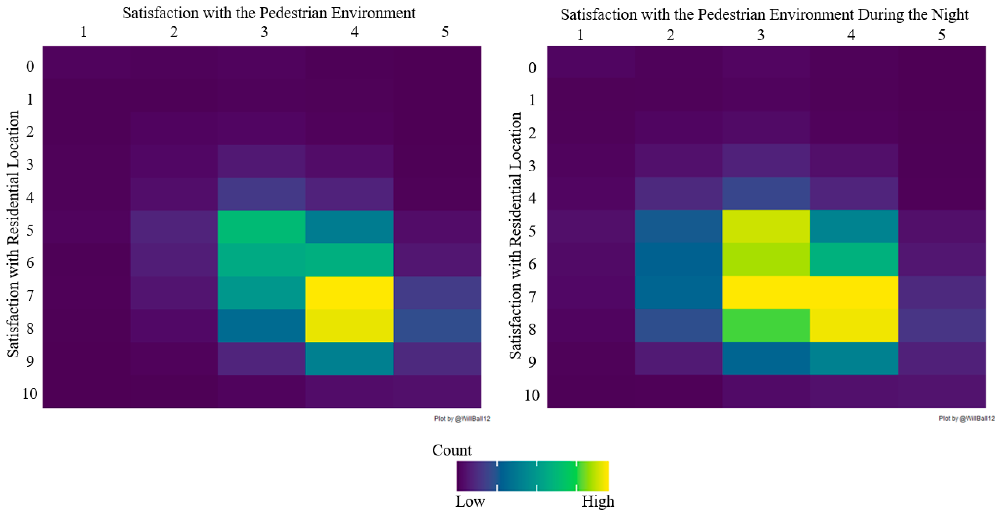
The satisfaction with the pedestrian environment in the neighborhood and the satisfaction with the pedestrian environment during the night in the neighborhood were the independent variables of interest in this study. We used both variables because pedestrian environments can differ between day and night depending on a variety of factors, such as perceived safety and street furniture. The two variables were operationalized using a Likert scale ranging from 1 (very dissatisfied) to 5 (very satisfied). Figure 1 visualizes a bivariate analysis between the dependent variable and two independent variables of interest. The plots suggest a strong correlation between the factors.

3.2.3. Control Variables

This study used several factors as control variables. For instance, this study controlled for several cognitive measures of neighborhood characteristics, such as respondents’ levels of satisfaction with the economic, social, and educational environments surrounding their residential location on a Likert scale. The final models also included an individuals’ level of satisfaction with their home and the surrounding infrastructure. In addition, the socio-demographic factors obtained from the survey were factored into the modeling as part of the process. The respondents’ gender, employment status, educational level, age, household income, and other relevant information were included in the analysis. There were nine features of housing or residence that needed to be controlled, such as the length of stay in Seoul, location of their neighborhood, and home ownership.

3.3. Analysis Methods

This study developed two models: (1) the proportional odds logistic regression and (2) gradient boosting decision tree models to answer the three research questions adequately. The two models used the same set of variables described in Table 2. Since this study employed a cross-sectional research design, it cannot establish causal inference. The following subsections offer details of the two models.

3.3.1. Proportional Odds Logistic Regression

This study utilized proportional odds logistic regression (POLR) (also called constrained cumulative logistic model) developed by McCullagh [17] and implemented through the R programming package. Since the dependent variable was an ordinal variable, POLR was appropriate since it is the generalized model of regression for ordinal data [18,19]. In detail, POLR analyzed the dependent variable as if it were a continuous variable and provided it with ten different cutoff points of increasing severity. Additionally, POLR allows the understanding of factors, such as satisfaction with the pedestrian environment, associated with a higher rating in satisfaction with residential location on a Likert scale. Moreover, POLR significantly improves the models’ interpretability by reducing the number of different coefficients for each ordinal category to a single coefficient for each independent variable. This reduces the number of coefficients significantly. To determine whether the final model adhered to the proportional odds assumption, this research used the Brant–Wald test [20]. The hypothesis of parallel regression was not validated by the results of the test at the p-value of 0.05.

3.3.2. Gradient Boosting Decision Tree Regressor

This study then used gradient boosting decision tree regressor (GBDT) using Python programming language to explore feature importance and non-linear relationship between factors and dependent variable. This study selected GBDT from among nine machine learning algorithms mainly due to its model performance. Regarding algorithm selection, the candidate models included linear regression (LR), support vector machine (SVM), decision tree (DT), random forest (RF), ada boosting decision tree (ADA), gradient boosting decision tree (GBDT), cat gradient boosting decision tree (CGBDT), stochastic gradient boosting decision tree (SGBDT), and extreme gradient boosting decision tree (XGBDT) models. A brief discussion of each algorithm can be found in

Table 3. Description of candidate machine learning algorithms [22] (pp. 154–155).

Algorithms	Brief Description
LR	LR deals with linear functions of the input features on the outcome target. LR usually serves as a baseline regressor in machine learning.
SVM	SVM finds a separating linear decision boundary called hyperplane (optimal decision surface) that maximizes the distance between data points [23].
DT	DT is used to predict a classification outcome by splitting training data based on the splitter for input features [24]. DT runs a sequential and hierarchical decision based on features.
RF	RF fits the same underlying algorithm to each bootstrapped copy of the original training data and then creates a final prediction by averaging the predictions from the different copies [25].
ADA	Boosting trains multiple models with subsets of data in a sequential fashion. ADA begins by assigning equal initial weights to all training data for weak learning training and then adjusts the weight distribution based on the results of the prediction [26].
GBDT	GBDT is a decision tree approach that is iterative. Its weak learners have strong dependencies between one another and are trained through progressive iterations based on the residuals. The ultimate result is calculated by adding up the results of all weak learners [27].
SGBDT	SGBDT is a hybrid algorithm that takes advantage of bagging and boosting techniques to improve prediction accuracy [28]. Using the term "stochastic" means that a random percentage of training data points will be used for each iteration rather than using all of the data for training [29].
CGBDT	CGBDT introduces modified target-based statistics that allow for the utilization of the entire dataset for training while avoiding the possibility of overfitting by performing random permutations [30].
XGBDT	XGBDT is an upgraded version of the GBDT. It obtains the residual by using second-order Taylor expansion on the cost function and incorporates a regularization term to regulate the complexity of the model simultaneously [30].

Abbreviation: linear regression (LR), support vector machine (SVM), decision tree (DT), random forest (RF), ada boosting decision tree (ADA), gradient boosting decision tree (GBDT), cat gradient boosting decision tree (CGBDT), stochastic gradient boosting decision tree (SGBDT), extreme gradient boosting decision tree (XGBDT) models.

. For hyper-parameter tuning, such as the maximum depth of the tree in DT, this study used the grid-search approach [21]. With the selected hyper-parameter tuning, this research trained the nine algorithms. Additionally, this study used the ordinal encoding using the sklearn package in Python to handle ordinal variables. Then, this study utilized negative mean absolute error, R-squared, and explained variance with the 10-fold cross-validation for model validation.

As shown in

Table 4. Model performance in the 10-fold cross-validation.

Model	Negative Mean Absolute Error		R Squared		Explained Variance
	Mean	Std	Mean	Std	Mean	Std
LR	−0.919	0.026	0.247	0.012	0.248	0.012
SVM	−0.898	0.028	0.104	0.047	0.111	0.048
DT	−0.909	0.031	0.246	0.019	0.247	0.020
RF	−0.857	0.026	0.319	0.013	0.321	0.013
ADA	−0.902	0.030	0.266	0.016	0.268	0.017
GBDT	−0.847	0.022	0.342	0.009	0.343	0.009
SGBDT	−0.868	0.023	0.309	0.011	0.310	0.011
CGBDT	−0.853	0.017	0.325	0.016	0.326	0.016
XGBDT	−0.853	0.022	0.327	0.017	0.328	0.017

Abbreviation: linear regression (LR), support vector machine (SVM), decision tree (DT), random forest (RF), ada boosting decision tree (ADA), gradient boosting decision tree (GBDT), cat gradient boosting decision tree (CGBDT), stochastic gradient boosting decision tree (SGBDT), extreme gradient boosting decision tree (XGBDT) models.

, GBDT showed the lowest negative mean absolute error and the highest R-squared and explained variance. Additionally, the results indicate that ensemble models, such as SGBR and XGB, significantly improved the prediction accuracy compared to the white machine learning algorithms, such as LR, SVM, and DT. Therefore, this study chose GBDT as the optimal algorithm and used it for further investigation.

Using GBDT, this study utilized two global model-agnostic ways of Explainable AI [31,32]: (1) feature importance [33] and (2) partial dependence plot [34] to answer the second and third research questions. First, this study used feature importance, which demonstrates variable importance by calculating the relative magnitude of the influence of the independent variables on prediction [35,36,37]. Specifically, it compares and ranks all input features that contribute to the reduction in the overall performance matrix [38]. This study computed both impurity-based and permutation-based feature importance. Second, this study employed a partial dependence plot (PDP) that estimates the expected effects of a particular variable on the dependent variable after controlling the influences of other factors [39,40,41].

4. Results

This section was divided into three subsections corresponding to each of the three research questions: (1) results of proportional odds logistic regression (POLR), (2) feature importance of gradient boosting decision tree regressor (GBDT), and (3) partial dependence plot of GBDT.

4.1. Proportional Odds Logistic Regression

Building on the bivariate analysis in Figure 1, this study developed additional insights through the estimation of the proportional odds logistic regression (POLR) model using the Likert-scale response of satisfaction with their neighborhoods as the dependent variable. The final model showed the McFadden R-squared of 0.079, CoxSnell score of 0.235, and Nagelkerke score of 0.243 (see

Table 5. Results of the final proportional odds logistic regression model.

Variables	Value	Std. Err	T-Value	p-Value	Odds Ratio
st_ped (reference: 1. very dissatisfied)
2. dissatisfied	0.068	0.312	0.219	0.827	1.071
3. neutral	0.068	0.307	0.222	0.825	1.070
4. satisfied	0.565	0.307	1.839	0.066	1.759
5. very satisfied	0.614	0.309	1.984	0.047	1.847
st_ped_n (reference: 1. very dissatisfied)
2. dissatisfied	0.516	0.097	5.304	0.000	1.675
3. neutral	0.594	0.095	6.250	0.000	1.812
4. satisfied	0.685	0.096	7.123	0.000	1.983
5. very satisfied	0.693	0.113	6.126	0.000	1.999
st_econ (reference: 1. very dissatisfied)
2. dissatisfied	0.020	0.081	0.251	0.802	1.021
3. neutral	0.086	0.079	1.084	0.278	1.089
4. satisfied	0.006	0.081	0.075	0.940	1.006
5. very satisfied	−0.040	0.094	−0.427	0.669	0.960
st_soci (reference: 1. very dissatisfied)
2. dissatisfied	0.016	0.124	0.132	0.895	1.016
3. neutral	0.044	0.123	0.360	0.719	1.045
4. satisfied	0.059	0.124	0.475	0.635	1.061
5. very satisfied	−0.014	0.133	−0.108	0.914	0.986
st_educ (reference: 1. very dissatisfied)
2. dissatisfied	0.085	0.110	0.770	0.441	1.089
3. neutral	0.106	0.108	0.978	0.328	1.112
4. satisfied	0.065	0.111	0.587	0.557	1.067
5. very satisfied	0.024	0.123	0.193	0.847	1.024
st_home (reference: 1. very dissatisfied)
2. dissatisfied	0.668	0.389	1.717	0.086	1.951
3. neutral	1.423	0.384	3.703	0.000	4.150
4. satisfied	2.078	0.385	5.403	0.000	7.991
5. very satisfied	2.958	0.387	7.642	0.000	19.265
st_infra (reference: 1. very dissatisfied)
2. dissatisfied	2.709	0.765	3.541	0.000	15.016
3. neutral	2.126	0.762	2.790	0.005	8.383
4. satisfied	2.848	0.762	3.736	0.000	17.260
5. very satisfied	3.206	0.763	4.200	0.000	24.692
male (ref: 0. no)	−0.077	0.028	−2.798	0.005	0.926
married (ref: 0. no)	0.137	0.035	3.956	0.000	1.147
age (reference: 1. 10~19)
2. 20~29	−0.050	0.085	−0.593	0.553	0.951
3. 30~39	−0.182	0.088	−2.069	0.039	0.834
4. 40~49	−0.262	0.090	−2.921	0.003	0.770
5. 50~59	−0.417	0.088	−4.726	0.000	0.659
6. over 60	−0.390	0.088	−4.417	0.000	0.677
edu (reference: 1. less than high school)
2. high school	0.356	0.055	6.488	0.000	1.428
3. college or bachelor	0.376	0.061	6.121	0.000	1.456
4. graduate school	0.591	0.156	3.789	0.000	1.806
hh_inc (reference: 1. less than KRW 1,000,000)
2. KRW 1,000,000~KRW 2,000,000	0.600	0.359	1.670	0.095	1.823
3. KRW 2,000,000~KRW 3,000,000	0.711	0.350	2.029	0.043	2.036
4. KRW 3,000,000~KRW 4,000,000	1.077	0.349	3.083	0.002	2.936
5. KRW 4,000,000~KRW 5,000,000	1.106	0.349	3.165	0.002	3.022
6. KRW 5,000,000~KRW 6,000,000	0.903	0.350	2.580	0.010	2.467
7. KRW 6,000,000~KRW 7,000,000	1.015	0.350	2.901	0.004	2.760
8. KRW 7,000,000~KRW 8,000,000	1.289	0.351	3.677	0.000	3.629
9. KRW 8,000,000~KRW 9,000,000	1.304	0.352	3.703	0.000	3.685
10. over KRW 9,000,000	1.436	0.352	4.080	0.000	4.203
OWN_HOME (ref: 0. no)	0.144	0.029	4.928	0.000	1.155
APT (ref: 0. no)	−0.076	0.030	−2.529	0.011	0.926
SFR (ref: 0. no)	0.067	0.035	1.898	0.058	1.069
resi_dt (ref: 0. no)	−0.345	0.054	−6.396	0.000	0.709
resi_en (ref: 0. no)	−0.118	0.039	−2.988	0.003	0.889
resi_wn (ref: 0. no)	−0.035	0.048	−0.741	0.459	0.965
resi_ws (ref: 0. no)	−0.453	0.040	−11.437	0.000	0.636
job_pro (ref: 0. no)	0.016	0.058	0.284	0.777	1.016
job_white (ref: 0. no)	0.077	0.038	2.046	0.041	1.080
job_blue (ref: 0. no)	−0.049	0.039	−1.253	0.210	0.952
disab (ref: 0. no)	−0.432	0.118	−3.651	0.000	0.649
hl_seoul	0.006	0.001	5.351	0.000	1.006
hl_gu	−0.003	0.001	−1.885	0.059	0.997
Intercept
0|1	−1.908	0.927	−2.057	0.040
1|2	−0.982	0.876	−1.121	0.262
2|3	0.241	0.864	0.279	0.781
3|4	1.830	0.863	2.119	0.034
4|5	3.405	0.865	3.937	0.000
5|6	4.826	0.865	5.576	0.000
6|7	6.091	0.866	7.035	0.000
7|8	7.448	0.866	8.600	0.000
8|9	9.219	0.866	10.642	0.000
9|10	12.353	0.870	14.196	0.000
Model Statistics
Observations	20,000
McFadden	0.079
CoxSnell Score	0.235
Nagelkerke Score	0.243
AIC	62,889.630

). Table 5 presents the estimates, standard error, T-value, p-value, and odds ratio of the final POLR model.

There are several notable findings. First, a higher score on satisfaction with the pedestrian environments in their neighborhoods (‘very satisfied’) significantly increased the odds of higher satisfaction levels with their neighborhood (estimate of 0.614 and odds ratio of 1.847). Additionally, satisfaction with the pedestrian environments during the night was also found to have significant effects on the dependent variable. Second, there was no significant correlation between the respondents’ levels of satisfaction with the economic, social, and educational environments in their neighborhoods and the dependent variable, although previous research has suggested that residents’ levels of satisfaction with their neighborhoods would increase over time because of their increased social capital, participation in economic activities, and utilization of education facilities. Third, the magnitudes of two variables, including satisfaction with their home and infrastructures in their neighborhoods, were the biggest among others. As expected, the associations were positive. Fourth, socio-demographic characteristics, such as gender, marital status, age, education attainment, household income, and home ownership, were also significant correlates of the dependent variable. For instance, being married increased the odds of the dependent variable with an odds ratio of 0.147. Additionally, the coefficient of the length of stay in Gu (administrative boundary in Seoul) was negative (estimate of −0.003) and marginally significant (p-value of 0.059), indicating that their life-cycle changes may render the community functions inadequate as their length of stay increases, which may lead to a drop in the level of satisfaction they have with the area.

4.2. Gradient Boosting Decision Tree Regressor

4.2.1. Feature Importance

This study developed a gradient boosting decision tree regressor model (GBDT) with the degree to which study participants were satisfied with the neighborhood in which they lived as the output target to identify which factors were most influential in predicting the level of satisfaction while controlling for other variables. The results of the impurity-based feature importance (IBFI) and the permutation-based feature importance (PBFI) are presented in

Table 6. Feature importance.

Variables	Impurity-Based Feature Importance		Permutation-Based Feature Importance
	Magnitude	Rank	Magnitude	Rank
st_ped	0.068	5	0.103	3
st_ped_n	0.048	7	0.057	6
st_econ	0.035	9	0.003	20
st_soci	0.033	10	0.002	22
st_educ	0.032	11	0.000	26
st_home	0.156	1	0.299	1
st_infra	0.110	2	0.178	2
male	0.016	17	0.001	24
married	0.015	18	0.007	17
job_pro	0.010	24	0.001	24
job_white	0.013	21	0.008	15
job_blue	0.013	21	0.006	18
disab	0.004	26	0.002	22
age	0.044	8	0.029	10
edu	0.023	12	0.009	14
hh_inc	0.064	6	0.064	4
OWN_HOME	0.018	14	0.012	13
APT	0.018	14	0.005	19
SFR	0.015	18	0.008	15
resi_dt	0.007	25	0.003	20
resi_en	0.017	16	0.030	9
resi_wn	0.012	23	0.024	11
resi_ws	0.020	13	0.044	7
resi_es	0.014	20	0.016	12
hl_seoul	0.103	3	0.031	8
hl_gu	0.093	4	0.061	5

, respectively.

It is interesting to note that respondents’ levels of satisfaction with pedestrian environments (st_ped) showed higher feature importance in the PBFI (10.3%) and IBFI (6.8%). With 5.7 percent in PBFI and 4.8 percent in IBFI, satisfaction with pedestrian environments during the night (st_ped_n) had lower feature importance than st_ped, but it still had higher feature importance than other variables. Additionally, a person’s level of satisfaction with their home (st_home), as well as their level of satisfaction with nearby infrastructure (st_infra), were the input features that had an exceptionally high level of importance for the prediction of a persons’ level of satisfaction with their residential location in both IBFI and PBFI. In addition, a persons’ level of satisfaction with their economic, social, and educational environments was found to have lower feature importance in comparison to other aspects. In addition, socio-demographic factors, which included household income, home ownership, age, and educational attainment, were found to be the influential factors associated with the satisfaction of residential location.

4.2.2. Partial Dependence

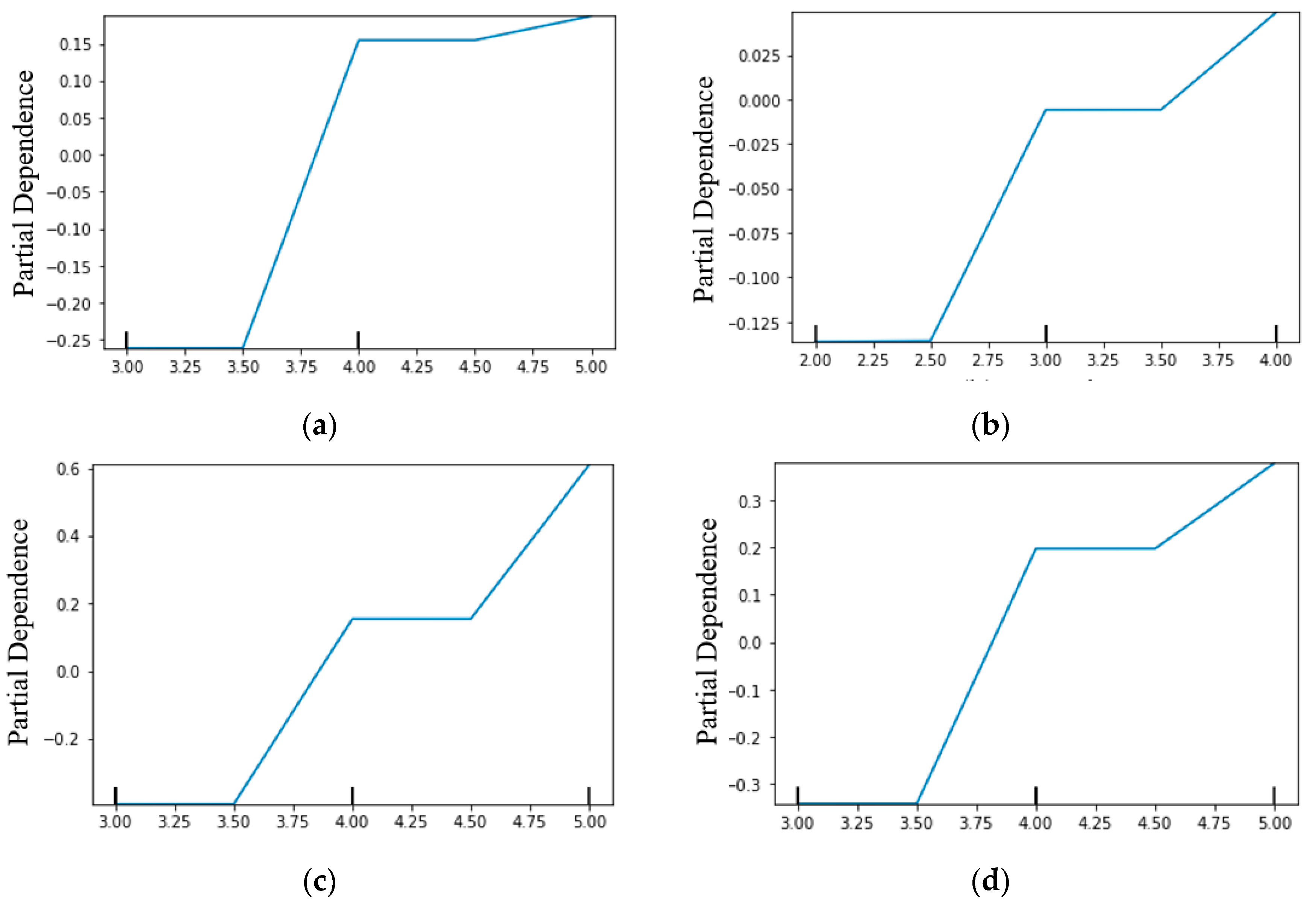
Figure 2 presents partial dependence plots (PDP), which compute the average prediction of an input feature on the output target using GBDT. PDP visualizes partial dependence [42] with a line graph. The curve in the PDP shows the average predicted effect of the input feature on the output target. In the line graph, the x-axis shows the values of the input features and the y-axis shows the corresponding PD. This subsection presents the PDP of two independent variables of interest and two influential factors found in the previous subsection.

Figure 2a shows that there was a consistent and negative relationship between a low level of satisfaction with the pedestrian environment in their neighborhoods and the dependent variable. However, the partial dependence on the dependent variable was significantly increased when respondents reported being satisfied or very satisfied with pedestrian environments. This can be seen in the fact that the partial dependence on the dependent variable increased when respondents reported being satisfied or very satisfied with pedestrian environments. Figure 2b shows similar patterns to Figure 2a; when respondents were satisfied or very satisfied with the pedestrian environment during the night, the degree to which study participants were satisfied with the neighborhood in which they lived significantly and rapidly increased. Figure 2c presents the PDP of the most influential factors found in the previous subsection. The plot suggests that the average degree of overall satisfaction with their neighborhood considerably increased as respondents were satisfied with their homes, while it remained stable and negative until the range. More interestingly, the magnitude of partial dependence was between –0.4 and 0.6, indicating the highest fluctuation among others. In Figure 2d, satisfaction with nearby infrastructures was significantly and non-linearly associated with the dependent variable.

5. Discussion

The key findings draw further discussions. First, consistent with the core hypotheses, the results of the two models together suggest that policymakers should recognize the importance and influence of satisfaction with the pedestrian environment in the neighborhoods on the degree to which individuals are satisfied with their neighborhood. That is, satisfaction with the pedestrian environment may be more than just users’ perceptions of the pedestrian level of services but also a critical factor influencing human lives. The conclusion may imply that pedestrian-friendly cities are not only essential for sustainable mobility [43] but also have direct implications beyond transportation, such as neighborhood satisfaction.

Another subject of further discussion is the finding that respondents’ degrees of satisfaction with pedestrian settings revealed greater feature importance than other elements. Transportation mode choice behavior in Seoul may explain the result.

Table 7. Transportation mode choice behaviors in Seoul [44].

	1996		2002		2006		2010
Active transportation	4,389,859	13.64%	5,230,690	14.98%	6,110,389	16.38%	6,499,084	17.26%
Vehicle	6,829,224	21.22%	7,982,832	22.87%	8,188,781	21.95%	7,501,988	19.92%
Taxi	2,901,178	9.01%	2,194,799	6.29%	1,959,612	5.25%	2,236,058	5.94%
Bus	8,357,730	25.96%	7,705,001	22.07%	8,616,326	23.10%	8,745,685	23.23%
Transit	8,182,634	25.42%	10,284,673	29.46%	10,839,341	29.05%	11,289,362	29.98%
Others	1,528,794	4.75%	1,512,971	4.33%	1,592,022	4.27%	1,382,479	3.67%
Total	32,189,419	100.00%	34,910,966	100.00%	37,306,471	100.00%	37,654,656	100.00%

Note: active transportation includes walking and bicycling.

indicates that the proportion of active transportation (i.e., walking and bicycling), bus, and transit in 2010 was 17.3%, 23.2%, and 30.0%, respectively [44]. More interestingly, the use of active transportation and transit increased between 1996 and 2010. The users of the transportation modes need better pedestrian environments, meaning they comprise nearly 70% of the total travel. Thus, pedestrian environments may be essential for many residents’ lives in Seoul, which may be reflected in the results of the feature importance.

Furthermore, this research endeavors to broaden its scope by incorporating earlier studies. The following recommendations are discussed to enhance the overall level of satisfaction with the pedestrian environment, which may, in turn, contribute to higher levels of neighborhood satisfaction. For instance, some of these include pedestrian-friendly street configurations related to the sidewalk, crosswalk, green space, street slope, and street furniture [45,46,47]. Another important dimension of the strategies can be related to the built environment, such as higher intersection density, mixed land use, and proximity to public transportation [48]. Additionally, other methods, such as strict regulations on illegal parking on the sidewalks and adequate safety systems for pedestrians, need to be considered. In addition, pedestrian environments are used by users of other modes of transportation, such as bicycles, micro-mobility services, wheelchairs, and baby strollers [49,50]. This means that pedestrian environments may not be exclusively for pedestrians, and policymakers should keep this in mind when formulating plans. The discussion is crucial since planners and policymakers should be aware of how to improve satisfaction with pedestrian environments, as this is tied to satisfaction with neighborhoods and, ultimately, individual well-being and sustainable urban environments.

6. Conclusions

Neighborhood satisfaction is a vital aspect of our lives. It has substantial implications for both policy and practice because it offers directions and recommendations for improving neighborhoods and, ultimately, the well-being of residents [5]. Although a body of literature has investigated the determinants of residents’ levels of satisfaction with their neighborhoods, empirical knowledge about the relationship between the degree to which individuals are satisfied with the neighborhood in which they live, and the level of satisfaction with pedestrian environments in their neighborhood is limited. Thus, this study employed proportional odds logistic regression and gradient boosting decision tree regressor models using the 2021 Seoul Urban Policy Indicator Survey. The key findings are as follows. First, there was a significant and positive relationship between the degree of satisfaction with the pedestrian environments in their neighborhoods and the degree of neighborhood satisfaction. Second, respondents’ satisfaction levels with pedestrian environments showed higher feature importance than other factors. Third, partial dependence plots demonstrate non-linear relationships; specifically, the partial dependence on the dependent variable was significantly increased when respondents reported being satisfied or very satisfied with pedestrian environments. The findings and discussions of this study can have important implications for framing policies to enhance neighborhood satisfaction through pedestrian environments. Additionally, this study was crucial since it may unfold what active mobility means to people and aid in developing effective, sustainable transportation planning frameworks. Ultimately, the author believes that the findings and discussions described here may be utilized to provide a means for improving the quality of life and creating sustainable urban environments.

The author acknowledges several limitations of this study. First, this study did not use essential factors regarding the built environment in the neighborhoods, such as mixed land use, urban form, and distance to the public transit station, during the modeling approach since the dataset did not offer the address of the respondents. Second, this study did not successfully reveal any causal mechanisms since this study employed cross-sectional analysis. Third, there is a limitation to this study since different population groups were not identified, and separate analyses were not conducted for each of these segments. Doing so would have helped better understand the various demands that different groups place on their neighborhoods. Fourth, this study did not examine the effect of COVID-19 on the results, although the survey was conducted in 2021. Fifth, the findings of this study may not be applicable to other study areas, such as regions with high single-occupant vehicle use. As such, the author highly recommends that future research handle the data limitations and explore the unanswered questions, such as whether COVID-19 has influenced the satisfaction of pedestrian environments and their neighborhoods.

References

- Campbell, A.; Converse, P.E.; Rodgers, W.L. The Quality of American Life: Perceptions, Evaluations, and Satisfactions; Russell Sage Foundation: New York, NY, USA, 1976; ISBN 978-1-61044-103-2. [Google Scholar]
- Diener, E.; Chan, M.Y. Happy People Live Longer: Subjective Well-Being Contributes to Health and Longevity. Appl. Psychol. Health Well Being 2011, 3, 1–43. [Google Scholar] [CrossRef]
- Kushlev, K.; Drummond, D.M.; Diener, E. Subjective Well-Being and Health Behaviors in 2.5 Million Americans. Appl. Psychol. Health Well Being 2020, 12, 166–187. [Google Scholar] [CrossRef] [PubMed]
- Cao, X.; Wu, X.; Yuan, Y. Examining Built Environmental Correlates of Neighborhood Satisfaction: A Focus on Analysis Approaches. J. Plan. Lit. 2018, 33, 419–432. [Google Scholar] [CrossRef]
- Marans, R.W.; Stimson, R.J. Investigating Quality of Urban Life: Theory, Methods, and Empirical Research; Springer Science & Business Media: New York, NY, USA, 2011; ISBN 978-94-007-1742-8. [Google Scholar]
- Yin, R.; Miao, X.; Geng, Z.; Sun, Y. Assessment of Residential Satisfaction and Influence Mechanism—A Case Study of Jinan City. J. Bus. Adm. Res. 2018, 7, 9. [Google Scholar] [CrossRef] [Green Version]
- Anton, C.E.; Lawrence, C. Home Is Where the Heart Is: The Effect of Place of Residence on Place Attachment and Community Participation. J. Environ. Psychol. 2014, 40, 451–461. [Google Scholar] [CrossRef] [Green Version]
- Putnam, R.D. Bowling Alone: America’s Declining Social Capital. In Culture and Politics: A Reader; Crothers, L., Lockhart, C., Eds.; Palgrave Macmillan US: New York, NY, USA, 2000; pp. 223–234. ISBN 978-1-349-62965-7. [Google Scholar]
- Yang, Y. A Tale of Two Cities: Physical Form and Neighborhood Satisfaction in Metropolitan Portland and Charlotte. J. Am. Plan. Assoc. 2008, 74, 307–323. [Google Scholar] [CrossRef]
- Lee, S.-W.; Ellis, C.D.; Kweon, B.-S.; Hong, S.-K. Relationship between Landscape Structure and Neighborhood Satisfaction in Urbanized Areas. Landsc. Urban Plan. 2008, 85, 60–70. [Google Scholar] [CrossRef]
- Hamersma, M.; Tillema, T.; Sussman, J.; Arts, J. Residential Satisfaction Close to Highways: The Impact of Accessibility, Nuisances and Highway Adjustment Projects. Transp. Res. Part A Policy Pract. 2014, 59, 106–121. [Google Scholar] [CrossRef] [Green Version]
- Lee, B.A.; Guest, A.M. Determinants of Neighborhood Satisfaction: A Metropolitan-Level Analysis. Sociol. Q. 1983, 24, 287–303. [Google Scholar] [CrossRef]
- Mouratidis, K. Neighborhood Characteristics, Neighborhood Satisfaction, and Well-Being: The Links with Neighborhood Deprivation. Land Use Policy 2020, 99, 104886. [Google Scholar] [CrossRef]
- Kim, J.W.; Lim, U. The Effect of Part-time Work on the Satisfaction of Personal Life—Using Seoul Survey. J. Korean Reg. Sci. Assoc. 2019, 35, 59–71. [Google Scholar] [CrossRef]
- Seoul Metropolitan Government. The 2021 Seoul Urban Policy Indicator Survey Final Report; Seoul Metropolitan Government: Seul, Korea, 2021. Available online: https://data.seoul.go.kr/dataList/OA-15564/F/1/datasetView.do (accessed on 30 June 2022).
- Subramanian, S.; Jones, V.; Duncan, C. Multilevel Methods for Public Health Research. In Neighborhoods and Health; Oxford University Press: Oxford, UK, 2003; ISBN 978-0-19-974792-4. [Google Scholar]
- McCullagh, P. Regression Models for Ordinal Data. J. R. Stat. Soc. Ser. B 1980, 42, 109–127. [Google Scholar] [CrossRef]
- Fagerland, M.W.; Hosmer, D.W. A Goodness-of-Fit Test for the Proportional Odds Regression Model. Stat. Med. 2013, 32, 2235–2249. [Google Scholar] [CrossRef] [PubMed]
- McNulty, K. Handbook of Regression Modeling in People Analytics: With Examples in R and Python; CRC Press: Boca Raton, FL, USA, 2021; ISBN 978-1-00-319415-6. [Google Scholar]
- Brant, R. Assessing Proportionality in the Proportional Odds Model for Ordinal Logistic Regression. Biometrics 1990, 46, 1171–1178. [Google Scholar] [CrossRef] [PubMed]
- Hillel, T.; Bierlaire, M.; Elshafie, M.Z.E.B.; Jin, Y. A Systematic Review of Machine Learning Classification Methodologies for Modelling Passenger Mode Choice. J. Choice Model. 2021, 38, 100221. [Google Scholar] [CrossRef]
- Lee, S. Transportation Mode Choice Behavior in the Era of Autonomous Vehicles: The Application of Discrete Choice Modeling and Machine Learning. Ph.D. Thesis, Portland State University, Portland, OR, USA, 2022. [Google Scholar]
- Cortes, C.; Vapnik, V. Support-Vector Networks. Mach. Learn. 1995, 20, 273–297. [Google Scholar] [CrossRef]
- Breiman, L.; Friedman, J.H.; Olshen, R.A.; Stone, C.J. Classification and Regression Trees; Routledge: Boca Raton, FL, USA, 2017; ISBN 978-1-315-13947-0. [Google Scholar]
- Bi, Q.; Goodman, K.E.; Kaminsky, J.; Lessler, J. What Is Machine Learning? A Primer for the Epidemiologist. Am. J. Epidemiol. 2019, 188, 2222–2239. [Google Scholar] [CrossRef]
- Azmi, S.S.; Baliga, S. An Overview of Boosting Decision Tree Algorithms Utilizing AdaBoost and XGBoost Boosting Strategies. Int. Res. J. Eng. Technol. 2020, 7, 5. [Google Scholar]
- Zhang, T.; He, W.; Zheng, H.; Cui, Y.; Song, H.; Fu, S. Satellite-Based Ground PM2.5 Estimation Using a Gradient Boosting Decision Tree. Chemosphere 2021, 268, 128801. [Google Scholar] [CrossRef] [PubMed]
- Zhou, J.; Shi, X.; Huang, R.; Qiu, X.; Chen, C. Feasibility of Stochastic Gradient Boosting Approach for Predicting Rockburst Damage in Burst-Prone Mines. Trans. Nonferrous Met. Soc. China 2016, 26, 1938–1945. [Google Scholar] [CrossRef]
- Nassif, A.B. Short Term Power Demand Prediction Using Stochastic Gradient Boosting. In Proceedings of the 2016 5th International Conference on Electronic Devices, Systems and Applications (ICEDSA), Ras Al Khaimah, United Arab Emirates, 6–8 December 2016; pp. 1–4. [Google Scholar]
- Wu, T.; Zhang, W.; Jiao, X.; Guo, W.; Hamoud, Y.A. Comparison of Five Boosting-Based Models for Estimating Daily Reference Evapotranspiration with Limited Meteorological Variables. PLoS ONE 2020, 15, e0235324. [Google Scholar] [CrossRef] [PubMed]
- Lee, S. Exploring Associations between Multimodality and Built Environment Characteristics in the U.S. Sustainability 2022, 14, 6629. [Google Scholar] [CrossRef]
- van Cranenburgh, S.; Wang, S.; Vij, A.; Pereira, F.; Walker, J. Choice Modelling in the Age of Machine Learning—Discussion Paper. J. Choice Model. 2022, 42, 100340. [Google Scholar] [CrossRef]
- Strobl, C.; Boulesteix, A.-L.; Zeileis, A.; Hothorn, T. Bias in Random Forest Variable Importance Measures: Illustrations, Sources and a Solution. BMC Bioinform. 2007, 8, 25. [Google Scholar] [CrossRef] [PubMed] [Green Version]
- Apley, D.W.; Zhu, J. Visualizing the Effects of Predictor Variables in Black Box Supervised Learning Models. J. R. Stat. Soc. Ser. B 2020, 82, 1059–1086. [Google Scholar] [CrossRef]
- Friedman, J.H. Greedy Function Approximation: A Gradient Boosting Machine. Ann. Stat. 2001, 29, 1189–1232. [Google Scholar] [CrossRef]
- Altmann, A.; Toloşi, L.; Sander, O.; Lengauer, T. Permutation Importance: A Corrected Feature Importance Measure. Bioinformatics 2010, 26, 1340–1347. [Google Scholar] [CrossRef] [PubMed]
- Huang, N.; Lu, G.; Xu, D. A Permutation Importance-Based Feature Selection Method for Short-Term Electricity Load Forecasting Using Random Forest. Energies 2016, 9, 767. [Google Scholar] [CrossRef] [Green Version]
- Zhou, Z.-H. Ensemble Methods: Foundations and Algorithms, 1st ed.; Chapman and Hall/CRC: Boca Raton, FL, USA, 2012; ISBN 978-1-4398-3003-1. [Google Scholar]
- Hastie, T.; Tibshirani, R.; Friedman, J. The Elements of Statistical Learning: Data Mining, Inference, and Prediction, 2nd ed.; Springer: New York, NY, USA, 2016; ISBN 978-0-387-84857-0. [Google Scholar]
- Lee, D.; Mulrow, J.; Haboucha, C.J.; Derrible, S.; Shiftan, Y. Attitudes on Autonomous Vehicle Adoption Using Interpretable Gradient Boosting Machine. Transp. Res. Rec. 2019, 2673, 865–878. [Google Scholar] [CrossRef]
- Molnar, C.; Freiesleben, T.; König, G.; Casalicchio, G.; Wright, M.N.; Bischl, B. Relating the Partial Dependence Plot and Permutation Feature Importance to the Data Generating Process. arXiv 2019, arXiv:2109.01433. [Google Scholar]
- Friedman, J.H. Multivariate Adaptive Regression Splines. Ann. Stat. 1991, 19, 1–67. [Google Scholar] [CrossRef]
- Guo, Z.; Loo, B.P.Y. Pedestrian Environment and Route Choice: Evidence from New York City and Hong Kong. J. Transp. Geogr. 2013, 28, 124–136. [Google Scholar] [CrossRef]
- The Seoul Research Data Service Transportation Mode Choice Patterns. Available online: https://data.si.re.kr/data/ (accessed on 13 July 2022).
- Kang, C.-D. The S + 5Ds: Spatial Access to Pedestrian Environments and Walking in Seoul, Korea. Cities 2018, 77, 130–141. [Google Scholar] [CrossRef]
- Lee, S.; Han, M.; Rhee, K.; Bae, B. Identification of Factors Affecting Pedestrian Satisfaction toward Land Use and Street Type. Sustainability 2021, 13, 10725. [Google Scholar] [CrossRef]
- Lee, J.; Kim, D.; Park, J. A Machine Learning and Computer Vision Study of the Environmental Characteristics of Streetscapes That Affect Pedestrian Satisfaction. Sustainability 2022, 14, 5730. [Google Scholar] [CrossRef]
- Kim, S.; Park, S.; Lee, J.S. Meso- or Micro-Scale? Environmental Factors Influencing Pedestrian Satisfaction. Transp. Res. Part D Transp. Environ. 2014, 30, 10–20. [Google Scholar] [CrossRef]
- Prescott, M.; Miller, W.C.; Borisoff, J.; Tan, P.; Garside, N.; Feick, R.; Mortenson, W.B. An Exploration of the Navigational Behaviours of People Who Use Wheeled Mobility Devices in Unfamiliar Pedestrian Environments. J. Transp. Health 2021, 20, 100975. [Google Scholar] [CrossRef]
- Lanza, K.; Burford, K.; Ganzar, L.A. Who Travels Where: Behavior of Pedestrians and Micromobility Users on Transportation Infrastructure. J. Transp. Geogr. 2022, 98, 103269. [Google Scholar] [CrossRef]
Figure 1.
Plots for Key Two Factors.
Figure 2.
Partial dependence plots for satisfaction-related factors. (a) st_ped; (b) st_ped_n; (c) st_home; (d) st_infra.