
Method for Assessing the Soundscape in a Marine Artificial Environment
by
 , , and
R. Benocci
1,* ,
,
E. Asnaghi
1,
A. Bisceglie
1,
S. Lavorano
2,
P. Galli
1,3 ,
,
H. E. Roman
4 and
and
G. Zambon
1 1
Department of Earth and Environmental Sciences (DISAT), University of Milano-Bicocca, Piazza della Scienza 1, 20126 Milano, Italy
2
Acquario di Genova-Costa Edutainment Area Porto Antico-Ponte Spinola, 16128 Genova, Italy
3
Dubai Business School, University of Dubai, Dubai P.O. Box 14143, United Arab Emirates
4
Department of Physics, University of Milano-Bicocca, Piazza della Scienza 3, 20126 Milano, Italy
*
Author to whom correspondence should be addressed.
Sustainability 2022, 14(16), 10359; https://0-doi-org.brum.beds.ac.uk/10.3390/su141610359
Submission received: 8 June 2022
/
Revised: 9 August 2022
/
Accepted: 13 August 2022
/
Published: 19 August 2022
(This article belongs to the Special Issue Soundscape: A Multidisciplinary Approach for Environmental Sustainability)
Abstract
:We applied standard acoustic methods to record, analyze and compare anthropogenic and biological signals belonging to the soundscape of artificial marine habitats. The study was conducted on two tanks located at the Acquario di Genova (Italy), the “Red Sea” and the “Tropical Lagoon” tanks, which represent different living environments hosting a variety of species and background sounds. The use of seven eco-acoustic indices, whose time series spanned the entire period of study, allowed the characterization of the environments. We investigated the extent to which eco-acoustic indices might describe the soundscape in an artificial marine environment surrounded by a background of mechanical noise, overlapping the diurnal/nocturnal fish chorusing produced by soniferous species. Three specific types of sounds emerged: (1) mechanical ones produced by the life-support system of the tanks; (2) anthropic origin ones due to maintenance and introduction of food; and (3) temporal trends associated with day/night cycles, especially impacted by artificial lighting. We searched for selected spectral patterns that were correlated to the time series of the eco-acoustic indices. The observed activity was found to be consistent with the sound emission of three specific fish species hosted in the tanks. The power spectral density (PSD) confirmed the presence of correlated signals (at 95th and 99th percentiles) for the identified frequency intervals. We expect that this method could be useful for studying the behavior of aquatic animals without intruding into their habitats.
1. Introduction
Landscapes and waterscapes are immersed in a blend of sounds characterizing a unique signature. Sounds produced by natural processes including the flow of water, wind, rain, or the sounds (calls and vocalizations) of animal species and even the faint signals produced by insects represent distinctive and unique elements for each habitat. The combination of these peculiarities yields a unique and characteristic “soundscape” for each habitat which should be preserved as close as possible to a pristine environment. In addition to these natural sounds, there are often present those produced by human activities, such as the noise of vehicles or other mechanical instruments (anthropophonies or technophonies) [1,2,3]. For this reason, the study of the soundscape, considering the distinctive characteristics of the environment, has benefited from the discipline of eco-acoustics; the latter has grown in importance and popularity as a non-invasive technique [4]. By looking into temporal and frequency patterns over long periods, eco- acoustics may be regarded as a tool to monitor the “composition” of the environmental sound, and of its possible temporal evolution, in particular when altered by external stresses such as pollution, climate change or the introduction of alien species [5]. However, eco-acoustics can be deemed as a discipline still under development, now increasingly being applied to investigate the biodiversity, habitat complexity and health of marine systems, with mixed results [6,7].
The aquatic environment can be affected by the influence of the adjacent terrestrial habitat; by the atmospheric and water temperature with cascading effects on stratification, oxygen concentrations and pH that vary according to depth and seasonality; and by light radiation that cannot propagate to great depths but concentrates near the water surface layers [8,9,10,11,12]. All these characteristics make aquatic habitats particularly changeable and difficult to investigate. However, increased water density facilitates the propagation of sound waves with respect to air-terrestrial environments due to increased sound speed, which makes sound frequencies prone to diffraction phenomena even at higher frequency [13]. This is why many water-living organisms have developed sound signatures as a specific communication tool [13]. Many marine aquatic species are able to take advantage of vocalizations, an observation that, over the years, has led to a rapid growth of marine bioacoustics [14,15].
Unfortunately, humans are increasingly contributing to acoustic pollution which may have profound impacts on the aquatic species lives [16]. For this reason, the Marine Strategy Framework Directive (MSFD) (2008/56/EC) [17] of the European Union consolidated the importance of marine bioacoustics, prompting action plans including earlier entry into the operation of programmes of measures to improve the marine environment. Eco-acoustics not only provides precious data to extend our knowledge on an environment, but it also plays an important role in taking protection actions [18]. It allows the characterization and quantification of the contributions of natural and anthropogenic sound sources and the recognition of ecological dynamics, all crucial elements for estimating the impact of anthropogenic perturbations on marine/aquatic settings [19].
A surge in applications of acoustic techniques has occurred mainly in terrestrial realms [20]. However, these acoustic techniques could also be successfully adopted to monitor fragile underwater ecosystems (lakes, coastal environments and oceanic coral reefs). In underwater and terrestrial ecosystems, a key advantage of acoustic-monitoring methods is the ability to record sound continuously [1,2]. In this regard, passive acoustic monitoring (PAM) changed this perspective, as it provides the unique opportunity to rapidly quantify and compare sound sources across habitats, space and time. Indeed, PAM has several advantages compared to traditional methods (e.g., visual field observations, satellite remote sensing, netting or electrofishing for the aquatic settings). It is mostly a non-invasive technique [3], allowing for collecting a great amount of data over long periods of time, enabling access to a greater range of habitats, especially in low-visibility environments (dense forests or underwater), and minimizing efforts and costs. These characteristics make PAM a complementary resource to be combined to remote sensing, which uses modern instruments including satellite, radar, as well as altimetry to study important ocean phenomena and processes.
It is known that eco-acoustic indices are able to capture different sound characteristics and, thus, highlight specific sound features. They are obtained through the post-processing of sound frequencies and levels to bring out specific characteristics of environmental sound. However, finding adequate and validated eco-acoustic indices, specifically for marine environments, is still an issue. In particular, the lack of universal indices or standardized protocols could lead to a potential misinterpretation caused by the use of different methods or addressing the effects of abiotic variables (such as, for example, daylight, tides, temperature, wind and earthquakes) either interfering with communications or influencing sound transmission [21]. The correlation between eco-acoustic indices and aural surveys is generally used to validate their robustness [22,23] and capability to derive information on the environmental quality [24]. This method is usually employed in terrestrial realms where the recognition of animal species is easier, and it is used with statistical analysis to generate spatial maps of environmental sound activity [25]. However, this approach is generally hindered in aquatic contexts, as the aural recognition of fish activity (mainly vocalization and foraging) is not easily distinguishable because of the inherent nature of the emitted sounds, generally characterized by short pulses (<0.1 s).
In this work, we aim to understand to what extent the above-mentioned procedure can be applied to marine enviroments, by considering a controlled artificial marine environment. To this end, measurements were performed at the public Acquario di Genova (Italy), where the “Red Sea” and the “Tropical Lagoon” tanks are located⋯ We assume, as our working hypothesis, that the eco-acoustic indices might display significant correlations with such an artificial marine environment soundscape, characterized by both high background mechanical noise and a conspicuous overlap of diurnal/nocturnal fish chorusing due to soniferous species. We computed seven eco-acoustic indices and we correlated the corresponding time series with biological and non-biological acoustic signals. By means of careful visual inspections, acoustic signals were obtained by selecting specific spectral patterns in sonograms. Such spectral cross-correlations allowed us to count the number of occurrences for each selected sound signal, showing that they were moderately correlated with the majority of the eco-acoustic indices. Specifically, we found that two spectral patterns, displaying both diurnal/nocturnal activity, were compatible with the sound emission of three identified fish species.
2. Material and Methods
2.1. Area of Study
The area of study involved two tanks of the Acquario di Genova, named “Tropical Lagoon” and “Red Sea”. The management policy of each tank requires that the man-made environment reproduces, as closely as possible, the natural one, in terms of the presence of plants and animal species.
2.1.1. “Tropical Lagoon” Tank
This tank is aimed at reproducing a typical habitat in the Indo-Pacific Ocean, a coral lagoon, characterized by a warm climate with a water temperature around (25–26) C, and includes a volume of 190 .
It is divided into two sectors: the first called the External Lagoon, dedicated to large animals such as the zebra shark (Stegostoma tigrinum), which feeds on fish and molluscs, and to the loggerhead sea turtle (Caretta caretta). The second, named Internal Lagoon, is dedicated to small fishes and corals. In the wild, the external lagoons, which are typical of the open sea, are characterized by deeper water, while the internal lagoons have shallower depths and, consequently, better lighting conditions. These characteristics provide proper conditions for the reproduction of many species of fishes and corals. Corals undoubtedly constitute a key element in this tank, and they are all captive-bred, reproduced by fragmentation techniques by the biologists of the aquarium. Their continuous reproduction inside the tropical tank gives rise to a real coral reef similar to the tropical natural ones. The most abundant fish species in the “Tropical Lagoon” (specifically in the Internal Lagoon) tank are the:
- Chromis viridis, also known as Green Damsel: this species is an extremely common marine fish. In nature, it is found in the Indo-Pacific region and spends much of its time in protected areas such as in coral-rich lagoons, from which it very rarely moves away. In the case of a reef suffering outbreak, this species moves in search of more suitable shelters, therefore representing an excellent indicator of the actual ecological status of coral reefs [26]. C. viridis produces click-like sounds during agonistic interactions. Most of the agonistic interactions and sound production were found to be directed to conspecifics (93.3%) [27]. The calls are produced in bursts of 1 to 22 clicks during chases. Very often, these chases ended in mutual parallel displays or in the fleeing of the chased fish. Clicks were most frequently single pulses, but they could be made up of two or more pulses [27].
- Clownfish, of which two species are hosted in the Lagoon: the Amphiprion ocellaris and the Amphiprion sandaracinos. During their life, these fishes give rise to a symbiotic bond with a specific group of anemones, which take on the function of protection for the eggs of the clownfish, while the latter bring them food [28]. The sound of this species was composed of single or a series of pulse sounds with stressed frequency component at 300–600 Hz and were composed of less than three pulses with wide frequency range (200–3500 Hz) with two or three stressed frequency component. A fish dashed toward the other fish floated in water and the sound was, sometimes, recorded just before passing each other [29].
2.1.2. “Red Sea” Tank
The “Red Sea” tank of the Acquario di Genova, dedicated to the reproduction of the “Red Sea” habitat, is a tank of 30 m volume. The most abundant species present in this tank are the:
- Pseudanthias squamipinnis, a pelagic spawner that feeds on zooplankton, whose maximum length is 15 cm. This species generally populates the coral outcrops, the reefs of the clear lagoons, the channels, and slopes. They are often territorial animals that tend to stay within 20 m from the rock or coral outcrop they have identified as a refuge. It is a hermaphroditic species and the gender transition from female to male is induced by the absence or removal of males from communities [30].
- Pseudochromis fridmani: this species, typical of the “Red Sea”, lives mainly in small caves, among the corals and debris on the reef slopes and on the drop-offs, at depths ranging from 3 m to 65 m. These specimens, endowed with a very shy character and a bright purple colour, live typically in pairs. Up to now, no significant population drops have been reported for this species in natural environments. However, due to its close affinity with coral reefs, increasingly threatened every day, it is likely that it could suffer a significant demographic decline in the near future [31,32,33].
- Dascyllus aruanus, commonly known as “white-tailed Damselfish”, is a species that, in nature, usually lives in large groups, up to about 30 individuals, sheltering among branched corals at depths from 1 m to 12 m. They leave their coral shelter solely to feed on zooplankton within the water column or to protect the territories where the young individuals are kept. One male can breed with several females, each laying up to 2000 eggs in the nest while, in the meantime, males aggressively guard the eggs and keep the nest clean of any debris. This species is known to live, under human care, at least nine years [34]. D. aruanus is known to produce two types of sounds, pops and chirps. The pop was produced during agonistic interactions when a specimen approached another’s shelter or during chases. A pop is generally composed of a single pulse. The peak frequency ranges from 680 Hz to 1300 Hz, with greater energy at the beginning of the sound. Pulses start with a low-frequency, low-amplitude half cycle, and increase immediately to a peak amplitude and frequency before starting to decrease in amplitude. Chirps are not associated with a specific behaviour and can function to announce the presence of the caller. They consist of trains of 12–42 pulses varying from 26 ms to 121 ms in duration, with an average pulse period of 48 ms. The peak frequency of the first band varied from 3400 Hz to 4100 Hz [35].
Among all the fish species present in both tanks, we found that, specifically, three fish species, namely: A. sandaracinos, C. viridis and D. aruanus, can produce a sound emission whose characteristics are summarized in Table 1.
In both tanks, keeping the level of oxygenation and purification of water at optimal levels requires a system for continuous circulation of water and filtering through mechanical pumps (life support system of the tanks consists of: filtration pumps, air pumps and biofilter outside the water and turbelle pump inside the water). This system inevitably produces vibrations and noise that become airborne and flank the tank structures. The mechanical noise is mainly concentrated at medium-low frequencies (<(3–4) kHz), and it is stationary. In order to reduce the impact of this mechanical component of the noise, we applied a high-pass filter to all the recordings with cut-off frequency = 4 kHz, as described by the following attenuation relation,
Besides the mechanical pumps noise, we had the lapping of water produced by the oxygenation system. This noise is mainly distributed at medium-high (3–20) kHz frequencies. The use of the filter altered the proportion of the noise components. The ordinary management operations in both tanks consist of feeding and cleaning activities, which often require divers to assure each species receives the right amount of food for its diet.
2.2. Instrumentation and Acquisition Scheme
The instrument used for underwater audio measurements is a bottom acoustic recorder named URec-384k (Dodotronic, made in Italy). It consists of an autonomous and programmable digital recorder, connected to a hydrophone with a maximum sampling rate of 384 kHz.
The sensor used in the measurement configuration is an Aquarian Scientific pre-amplified hydrophone AS-1, mounted on one cap. It is a calibrated unit with a receiving sensitivity of −208 dBV re 1 Pa (40 V/Pascal).
Two recording units URec-384k were used for the monitoring campaign at the Acquario di Genova, one for each tank. The optimal location of the instrument inside the tanks was identified by considering the capability to acquire the greatest number of biophonic emissions, without being excessively disturbed by human activities during the managements of the tanks. The recorders were placed at a depth of 1.5 m in both tanks.
The instrument was housed in a protective net, equipped with a floating ring and a weight. In this way, it was possible to fix the recorder at a specific depth and to prevent the fishes from getting too close to the instrument, hitting the sensor. The measurements finally used for our purposes (see Figure 1) were carried out during the following periods,
- 02/25/2021–03/12/2021: “Red Sea” tank monitoring.
- 06/10/2021–06/15/2021: “Tropical Lagoon” tank monitoring.
The acquisition patterns were 5 min recording and 10 min pause for the “Red Sea” tank, and 5 min recording and 1 min pause for the “Tropical Lagoon” tank. They were selected to optimize the total number of recordings, while also taking into account a balance between recording time and data storage capability. The two campaigns were conducted in different periods; this allowed us to fine-tune the measurement settings in the second campaign. The sampling rate for the measurements was set at 192 kHz and kept constant throughout the measurements.
2.3. Metrics for Acoustic Signal Analysis
We discuss first the calculation of the eco-acoustic indices followed by the principal acoustic metrics to characterize the environmental sound. The eco-acoustic indices are able to capture different sound characteristics and, thus, highlight specific sound features. The fast Fourier transform (FFT) algorithm is the basis for calculating different eco-acoustic indices. Indeed, these indices are obtained through post-processing of sound frequencies and levels to bring out specific characteristics of environmental sound. In the analysis, we used the following seven indices, chosen from a range of previous soundscape studies, with the specified frequency intervals, f, reported in Table 2. The Acoustic Complexity Index (ACI), which determines the modulation in intensity of a signal over changing frequencies; the Acoustic Diversity Index (ADI), which provides a measure of evenness across spectral frequencies; the Acoustic Evenness Index (AEI), which provides reverse information of ADI with high values identifying recordings with dominance of a narrow frequency band; the Bio-acoustic Index (BI), which provides the area under the mean frequency spectrum above a threshold characteristic of the biophonic activity; the Acoustic Entropy Index (H), which highlights the evenness of a signal’s amplitude over time and across the available range of frequencies; the Normalized Difference Soundscape Index (NDSI), which accounts for the the ratio between technophonies and biological acoustic signals; and the Dynamic Spectral Centroid (DSC), which indicates the centre of mass of the spectrum.
The analysis and computation of eco-acoustic indices were performed in “R” environment, version 3.5.1 [43]. In particular, the FFT analysis was computed by the function spectro, available in the R package “Seewave” [44] based on 2048 FFT points. The corresponding frequency bins, that is, the intervals between samples in frequency domain, are calculated by dividing the sampling rate (194 kHz in our case) by the number of FFT points (or FFT size). Thus, the latter value determines the frequency resolution. In our case, this is equivalent to a frequency bin (resolution) of F = 93.75 Hz (sampling rate/2048) and, therefore, a time resolution of s. This choice represents a compromise between a good temporal and frequency resolution. The R package “Soundecology” [45] was used for the indices computation with the exception of the Dynamic Spectral Centroid (DSC), for which a specific script was written. The frequency bounds were set between 100 Hz and 20 kHz. The latter was chosen after careful inspections of the recorded spectra (no signals were observed above the upper frequency limit of 20 kHz). The eco-acoustic indices were calculated with a time resolution equal to the time duration of the recordings (5 min). The Pearson’s correlation test was also used for the analyses.
There is also a wide variety of metrics used in the analysis of acoustic signals. One of the most commonly used metric is based on the Power Spectral Density (PSD) method. To this end, one considers a time series , representing the amplitude of the signal of interest, and calculates the power spectrum density of , describing the distribution of power associated with each frequency component of the signal [46]. The power spectrum (see, e.g., [47,48]) is defined according to,
where T is the length of the time series, and is the Fourier transform of the time convolution of the signal with itself in the form,
2.4. Pattern Recognition
In aquatic contexts, the aural recognition of fish activity (mainly vocalization and feeding), that is, the manual validation by listening to the recordings, is not straightforward because the emitted sounds are generally characterized by short pulses (<0.1 s). However, this difficulty is further worsened in artificial marine environments where the presence of mechanical disturbances strongly interfere or even overlap with biophonic activities, making the aural recognition by operators not viable (attempts did not bring to any satisfactory results). For this reason, we adopted spectral pattern recognition as validation method for the eco-acoustic indices. Thus, it represents a sort of automatically made aural-survey surrogate.
Characterizing the presence of different acoustic patterns in an audio recording can provide interesting information on the presence of animal vocalization or other specific activities such as feeding (see an example below). After “manually” selecting a spectral template within a Fourier-transformed representation (a spectrogram) of an audio recording, i.e., by visually inspecting spectrograms one at a time, the search was followed by a spectral cross-correlation approach. Thus, we looked at “similarities” between the spectral template and the spectrogram of the audio recording: namely, we considered as “similar”, spectra above a given cross-correlation coefficient. The analysis was carried out in R environment using the R package MonitoR [51]. This package allowed the creation, modification, saving and use of templates for pattern recognition. The matching between templates and spectra was based on a correlation threshold typically found by a trained and test/validation process. The package translates raw scores from template-matching to detection information, by finding peaks in the score data, and determining which peaks, if any, exceed the score cut-offs specified in the templates.
A small tank (dimensions 110 cm × 60 cm × 40 cm) containing two sea urchins (Diadema setosum) was used for the initial tests. In particular, the sound emission released by a single sea urchin was recorded during the feeding activity with a cabled hydrophone (URec-384k).
3. Results
3.1. Eco-Acoustic Indices
Figure 2 and Figure 3 show the time profile of ACI, ADI, AEI, DSC and H indices for the Lagoon and “Red Sea” tanks for the entire period of the measuring campaign (5 days for the “Tropical Lagoon” tank and 15 days for the “Red Sea” tank). In both Figure 2 and Figure 3, two coloured bands highlight the day intervals: yellow stripes correspond to the hours of the day in which the aquarium lighting system is kept in operation (from 8:00 a.m. to 7:00 p.m.), and night bands depicted in grey are where the lights are instead turned off (from 7:00 p.m. to 8:00 a.m.). Within the graphs of both tanks, a number of events have been marked as reported by the aquarium operators. The type of events was labelled as illustrated in Table 3. In this way, it was possible to find an explanation for many of the peaks highlighted by the indices.
Each index profile is able to highlight events such as: the feeding operations (C) that take place daily (indistinct noise with a duration of minutes), the presence of divers (S) that takes place periodically (indistinct noises with duration of minutes) or a disturbance linked to the use of a brush (D) used to carry out maintenance operations inside the tank (pulse trains with duration of minutes). In particular, some indices, such as ACI, BI and H, were able to highlight the onset of a disturbance similar to an electrical buzz (RE) (duration, several hours), which developed towards the end of the first measurement day. The RE were particularly constant in time, thus altering the heterogeneity of relative frequencies and their intensities. In addition, the presence visitors (V) was characterized by indistict noises, whereas the low pitch noise (LP) presented a series of pulses at low frequency with a duration of seconds. To be noted is that the change in the profile trend of BI index (see Figure 2a), starting from the second day of the measurement campaign, and right after the diving operations, is linked to the displacement of the hydrophone by divers. BI is more sensitive to noise level variations, implying that the sensor was placed at a greater distance from the noise source (pumps). Another important consideration is the quite-evident day/night periodic trend, which is especially picked up by BI, ACI, DSC and H indices.
The conclusions drawn for the “Tropical Lagoon” tank apply also to the “Red Sea” tank. Indeed, also in this case, the eco-acoustic indices highlighted how anthropic operations are able to condition the soundscape and show different trends between the night and day periods. In particular, by inspecting the graphs in Figure 3, it is possible to observe how the trend of DSC and H indices (see Figure 3e,f) during the ninth day of measurements, show significant change in the time profiles. This variation is justified by the operations that took place inside the tank: siphoning of the sand and immersion of the divers, who had to move the hydrophone.
As illustrated in Figure 2c,d and Figure 3c,d, ADI and AEI indices do not show any day/night trend but just underline maintenance activities in the form of peaks. For this reason, we decided to show the boxplots of the indices distribution just for ACI, DSC, BI and H (see Figure 4a,d). These illustrations allow highlighting of how the day/night period present similar distributions, but display slightly fewer values for the night period. As expected, most of outliers are concentrated during daytime (values outside the boundary of the whiskers). The two tanks are very different both in size and equipment (different hydraulic pumps and water oxygenation systems). These characteristics may contribute to generating distinct sound environments, which are reflected in the generally different values of the indices.
3.2. Results of Power Spectral Density
Here, we present the calculation of the PSD described in Section 2.3, for the mean levels recorded over the entire measurement campaign. The results are shown in Figure 5 for the “Tropical Lagoon” (upper panel) and the “Red Sea” (bottom panel) tanks. As is apparent, there is a large frequency interval, (300–4000) Hz, for which the 95th and 99th quantiles show a significant correlation.
Specifically, the “Tropical Lagoon” tank presents a larger broadband correlation which includes Pitch0, the noise associated with the hydraulic pumps and a peak at around 4 kHz. The latter was not found during the visual inspection of the spectrogram. The fact that the peaks associated with these frequencies emerge at 95th and 99th quantiles means that they are correlated with quite rare events. In addition, the hydraulic pump presents rare correlated frequencies when the majority of the distribution provide more correlated results.
As for the “Red Sea” tank, we can observe, within the same frequency interval, more noticeable events at approximately 300 Hz and 900 Hz, a series of near peaks around (1.5–3.0) kHz, plus a single peak at 15 kHz. In this case, Pitch0 can be identified with the peak centred at 900 Hz, Pitch 1 with the peak at about 3 kHz and Pitch 3 with the peak at about 15 kHz. The latter, being associated with the water lapping, may represent rare correlated events. The peak at 300 Hz was not found in the spectrograms, whereas the peaks near 2 kHz are due to the hydraulic pumps as for the “Tropical Lagoon” tank.
3.3. Results of Pattern Recognition
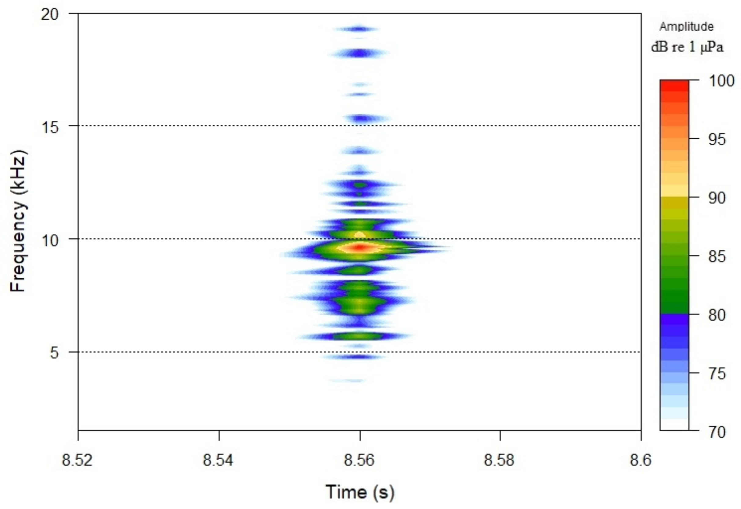
Testing the pattern-recognition algorithm described in Section 2.4, based on the cross-correlation between a spectral pattern and the entire spectrogram of the audio recording of 460 s duration, was performed using the sound emission released by a single sea urchin (Diadema setosum). Figure 6 shows the spectrogram peaked at approximately 10 kHz with a duration of less than 0.02 s. The repetition period of the signal is found to be about 5 s. The number of signals was counted for the entire recording and a correlation coefficient threshold was set in order to reproduce the number of counted signals. Figure 7a shows the sound events matching the spectral template of Figure 6, whereas Figure 7b returns information on all score peaks and those peaks that are considered detections (above 0.7 threshold). The time axis refers to an extract of the recording (from 400 s to 460 s). In Table 4, the results of the confusion matrix are reported. For the specified threshold we obtain: Accuray = (TP + TN)/(TP + TN + FP + FN) = 0.78, Sensitivity = (TP)/(TP + FP) = 0.84, Specificity = (TN)/(FP + TP) = 0.84, and a McNemar’s Test p-Value of 0.85 [52]. The latter result states that we cannot reject the null hypotheses, meaning that we have a good performance of the predicted occurrences.
After this first step, we identified in the audio recordings the four most abundant spectral templates ranging from approximately 1 kHz to 17 kHz. The identified spectral patterns, named pitches, are illustrated in Figure 8. Their characteristics are summarized in Table 5. To be noted is that all the pitches present a time duration s. This value represents the time resolution of the spectrogram as determined by the number of FFT points (2048) chosen for the FFT computation. This means that the pitch duration could be of an even lesser duration.
Based on the procedure illustrated in Section 2.4, for which the recognition of the sea urchin’s feeding-activity sound template was validated for a threshold correlation coefficient of 0.7, we decided to search for the different spectral templates (pitches) in the audio files following two steps:
- Varying the correlation coefficient threshold over a wider interval: from 0.3 to 0.7;
- Selecting the pitch time series obtained with the correlation coefficient threshold that better correlates the time series of the eco-acoustic indices.
In the first step, clearly, the number of matches (occurrences) in each recording increases by increasing the threshold. Indeed, assuming, for example, a Gaussian profile for the last three pitches (Pitch0 is excluded as it presents three peaks), one can verify that, for instance, correlation coefficients equal to 0.3 and 0.7 correspond to mean frequency variations around the main peak of about ±400 Hz and ±200 Hz, respectively. This means that considering, for instance, a correlation coefficient of 0.3, we will count, as Pitch1, Gaussian spectral profiles with maxima between 2.7 and 3.5 kHz. Higher correlation coefficients correspond to higher selectivity. Thus, each correlation coefficient determines a time series of events. In order to define an “optimal” correlation coefficient threshold, we decided to calculate the Pearson’s cross-correlation among the computed eco-acoustic indices, generally correlated to the presence of sound activities (both biophonies and technophonies), and the time series of events. We also included the time series of the equivalent sound level calculated over the entire recording period of 5 min, . Table 6 and Table 7 report the “optimal” Pearson’s correlation coefficients among eco-acoustic indices, , and pitch time series for the “Tropical Lagoon” and “Red Sea” tanks, respectively, where the pitch time series for the “Tropical Lagoon” tank has been obtained with a spectral correlation coefficient threshold of 0.4 and the pitch time series for the “Red Sea” tank with a spectral correlation coefficient threshold of 0.5.
As is apparent, the threshold values 0.4 and 0.5 seem to match our requirements for the “Tropical Lagoon” and the “Red Sea” tanks, respectively. As for the Tropical Lagoon tank, we can observe that, for a correlation coefficient threshold of 0.4:
- Pitch0 is moderately correlated with the ACI time series (0.51), with ADI (−0.47) with AEI (0.45) and (−0.35);
- Pitch1 is moderately correlated with the BI time series (−0.59) and with H (0.43);
- Pitch2 is moderately correlated with the ACI time series (0.39);
- Pitch3 is weakly correlated with all indices.
As for the “Red Sea” tank, we can observe that, for a correlation coefficient threshold of 0.5:
- Pitch0 is moderately correlated with the ADI time series(−0.56), with AEI (0.52), with DSC (−0.45), with ACI (0.38) and (−0.30);
- Pitch1 is moderately correlated with the H time series (−0.63), with ACI (0.42) and ADI/AEI (0.39);
- Pitch2 is moderately correlated with the ACI time series (0.67);
- Pitch3 is weakly correlated with all indices.
In particular, Pitch0 and Pitch1 present a mild correlation with the higher number of eco-acoustic indices (2–4 indices); Pitch2 is moderately correlated with just a single index and Pitch3 turns out to be not correlated with any index time series. To be noted is that pitches are just weakly correlated with each other in the “Red Sea” tank. This means that there is a weak positive relationship between their time series. Instead, their correlation with the computed eco-acoustic indices is moderate meaning that they are are sensitive to the identified spectral patterns.
Figure 9 and Figure 10 report the hourly median normalized occurrences for the four-pitch templates found in the “Tropical Lagoon” tank using a correlation coefficient threshold of 0.4 and in the “Red Sea” tank using a correlation coefficient threshold of 0.5. The normalization was carried out with respect to the median value and the coloured bands represent the median absolute deviation (MAD).
In both figures, we can observe how the Pitch0 profile is the only spectral pattern among the four categories showing a significant positive deviation from the median value during the period (6:00 a.m.–4:00 p.m.) for the “Tropical Lagoon” tank and (6:00–10:00) a.m. and (4:00–6:00) p.m. for the “Red Sea” tank. This means that, in these time intervals, we detected an increase in Pitch0 activity. To be noted is the high MAD of Pitch0, which reflects the higher variability of this spectral pattern.
4. Discussion
Eco-acoustic indices have shown a rather good accuracy in measuring species diversity in some environments [37,40,53]. Animal species produce a plethora of sounds and this acoustic diversity can be used to extract information on species richness [3,37,40,53]. Nonetheless, this relationship is not always straightforward [54].
The results shown in Section 3 reveal the good capability of the eco-acoustic indices to discriminate among different activities, especially antropophonic and technophonic ones, consistent with the empirical observations by the aquarium operators (cf. Figure 2 and Figure 3 and Table 3). Nevertheless, Figure 2 and Figure 3 highlight the presence of day/night trends in some of the eco-acoustic indices profiles.
The circadian patterns recorded in this work are consistent with data from other studies [19,55], in which fish choruses are especially active at dawn and at dusk. These specific patterns are captured by, mainly, the BI, ACI, AEI DSC and H indices. More specifically, it seems that BI, ACI, ADI and AEI are more sensitive to both biophonic and anthropophonic sounds. As is apparent, the ADI index is only activated by anthropophonic sounds. On the other hand, DCS and H seem to show a more pronounced circadian pattern, typical of biophonic activities. Calibration of eco-acoustic indices in different habitats has been reported in a number of studies, showing, for instance, that bird responces to restoration efforts in forests have been properly described by the acoustic entropy, H. Conversely, the M and ACI indices could capture significant activity variations in floodplains [56,57].
Eco-acoustic indices can help identify different sound compositions but they appear to need adjustment in artificial environments as compared with wild marine environments due to low signal-to-noise ratio. In this context, audio filtering can potentally enhance sounds of interest. The observed circadian dynamics suggested searching for biophonic sound sources in the audio recordings. As illustrated in Section 3.3, observing the spectrogram of the recordings, four spectral templates (pitches) were selected and the time series of the corresponding occurrences were found. In addition, the observation of a moderate correlation among the eco-acoustic indices and Pitch0 and Pitch1 indicated that their spectral patterns were picked up by those metrics.
The results obtained for the cross-correlation among the computed eco-acoustic indices and the time series of events illustrated in Table 6 and Table 7 show that Pitch0 in the “Tropical Lagoon” tank is correlated with those indices expression of frequency modulation (ACI) and anticorrelated with ADI representing entropy in frequency space meaning that the presence of Pitch0 is “favoured” by the absence of other sound frequencies (higher frequencies). As for the “Red Sea” tank, Pitch0 shows the same correlation pattern with the addition of an anticorrelation with DSC index, meaning that an increase in activity corresponds to a decrease in the frequency content in the recordings. The latter could be associated with either the frequency content of Pitch0 or the reduction in other high-frequency sources. Only Pitch0 is moderately anticorrelated with in both tanks.
A weak increase in Pitch1 activity is also observed for the “Red Sea” tank in the interval (1:00 and 4:00) a.m. In this case, Pitch1 is anticorrelated (moderately) with H which measures entropy in both time and frequency space and is correlated (moderately) with ADI. This suggests an unevenness in time (which is dominant for H) and evenness in frequency domain. Additionally, for this pitch, we observe a correlation with ACI. In this case, Pitch1, but especially Pitch2 and Pitch3, present a lower MAD and are concentrated around the median value. Hence, these pattern characteristics are typical of stationary sounds all over the clock and might be associated with sounds of a mechanical nature.
For these reasons, we are more prone to consider Pitch0 as a sound associated with biophonic activity than the other pitches. The moderate anticorrelation with may suggest that fish chorusing is more likely to be observed with overall decreasing background noise. Looking at the sound emission characteristics of A. sandaracinos, C. viridis, and D. aruanus presented in Table 1, we could reasonably recognize a likelihood between Pitch0 and the emission interval of these species (their reported emission interval contains Pitch0).
The present study was performed in a controlled area, but the presence of a high background mechanical noise introduced a bias in the analysis that hampered a strong association between biophonic activity and eco-acoustic indices, despite our attempt to reduce its impact by using a high-pass filter. For this reason, we excluded the NDSI index. In fact, although it has been introduced in terrestrial habitats to weigh the contribution of biophonies and anthropogenic noise, in marine habitats it can be applied to weigh the contribution of two different biophonies: fish emitting at quite low frequencies (generally up to 1 kHz [58]) and invertebrates with peak spectrum between 2 kHz and 5 kHz [59].
An important issue requiring further investigation is to what extent acoustic indices relate to the aquatic fauna in the habitats from which they are derived and whether they are affected by other sources of different spectral or temporal content. This represents a key point, as ecoacoustic indices allow fast assessment of long audio recordings as compared to other time-consuming spectral analysis. This characteristic is particularly important as the spread of PAM has made available cost-effective, unattended and non-invasive acoustic sampling over extended periods of time, thus helping capture changes in soundscape and biodiversity due to climate change and human intrusion. Indeed, little is known about the impacts of the sounds of anthropogenic activities on aquatic wildlife, or their physiological effects, which may affect the fitness of individuals, populations, or even whole communities of animals [60].
The method of pattern recognition based on spectral cross-correlation has been used to mimic what, in terrestrial realms, is usually referred to as an aural survey. The method allows quick detection of specific spectral patterns but it needs further refinements in terms of defining an optimal cross-correlation coefficient threshold accounting for possible variation in the emitted sound. Due to the non-automatic search of spectral patterns, events less likely to happen are hardly found. A validation of this method with acoustic measurements of marine organisms in their wild habitats will help refine this tool. With proper tuning, this method could help the study of the behavior of aquatic animals without intruding into their habitats.
5. Conclusions
In this paper, we report the results of measurements and analysis of sound recordings carried out at two different artificial and controlled marine environments, the “Red Sea” and the “Tropical Lagoon” tanks located within the Acquario di Genova, Italy. The present study was performed in a controlled area but the presence of high background mechanical noise introduced a bias in the analysis that hampered a strong association between biophonic activity and eco-acoustic indices. The initial hypothesis that the eco-acoustic indices might correlate the soundscape in an artificial marine environment characterized by a high background mechanical noise with an overlapped diurnal/nocturnal fish chorusing by soniferous species was answered, even minimally, by measuring, analyzing and comparing biological acoustic signals produced by organisms present in two different artificial marine habitats.
We computed seven eco-acoustic indices and correlated the corresponding time series with biological and non-biological acoustic signals. Acoustic signals were obtained by selecting specific spectral patterns in the sonograms following a careful visual inspection.“Spectral Cross Correlation” allowed counting the occurrences for each selected sound signal, thus showing how those signals, displaying a variation in activity throughout the day, were moderately correlated with the majority of eco-acoustic indices. We found that two spectral patterns, with diurnal/nocturnal activity, are compatible with the sound emissions of three fish species.
Thus, the use of both spectral analysis and the time profile of seven eco-acoustic indices highlighted three specific features: (1) the presence of mechanical sounds produced by the hydraulic pumps and the oxygenation system; (2) the presence of anthropophonic sounds (maintenance and feeding activity during daytime); and (3) the presence of a periodicity associated with day/night cycles.
To make the analysis less affected by the high background noise, a high-pass filter with = 4 kHz was applied. Aural surveys were usually employed to validate the analysis but, in this specific case, the presence of background noise and the impulsive nature of biophonies, lacking a frequency modulation, hampered this task. A validation methodology was implemented by identifying four spectral patterns within the recordings, denoted as: Pitch0 (three peaks at 0.5 kHz, 0.9 kHz, 1.2 kHz), Pitch1 (peak at 3.1 kHz), Pitch2 (peak at 7.4 kHz), and Pitch3 (peak at 15.2 kHz). Spectral cross-correlations allowed searching for these spectral templates, and the corresponding matches (number of events found in each recording) were correlated with the time series of the eco-acoustic indices. In particular, two pitches, Pitch0 and Pitch1, showed a moderate correlation with the eco-acoustic indices. The hourly median time profile of Pitch0 occurrences showed an increase in counts during the period (6:00 a.m.–4:00 p.m.) for the “Tropical Lagoon” tank, and during (6:00–10:00) a.m. and (4:00–6:00) p.m. for the “Red Sea” tank. The sound pattern associated with Pitch0 is compatible with the sound emission of three fish species, i.e., A. sandaracinos and C. viridis present in the “Tropical Lagoon” tank, and D. aruanus in the “Red Sea” tanks. The other sound pitches are characterized by a lower variability and stationarity, typical of mechanically produced sounds.
PSD revealed the presence of active frequency bands at the 95th and 99th quantiles. These correspond either to correlated events produced by biophonic activities, or rare recurring events which are generally uncorrelated (e.g., water lapping). Despite the presence of a high noise-to-signal ratio, the proposed method was able to highlight biophonic activities, likely due to the two fish species A. sandaracinos and C. viridis, by combining the information carried by the time series of the computed eco-acoustic indices and the use of spectral patterns. This procedure, though promising, requires to be tested in wild environments, where background noise has generally much less impact, in order to properly define the set of eco-acoustic indices that are significantly correlated with the biophonic activities.
Author Contributions
Conceptualization, R.B. and G.Z.; methodology, R.B.; software, R.B. and E.A.; formal analysis, R.B. and E.A.; investigation, R.B.; resources, G.Z.; data curation, A.B. and E.A.; writing—original draft preparation, R.B.; writing—review and editing, R.B., H.E.R. and G.Z.; visualization, R.B., E.A. and H.E.R.; project administration, G.Z., P.G. and S.L.; funding acquisition, G.Z. and P.G. All authors have read and agreed to the published version of the manuscript.
Funding
This research received no external funding.
Data Availability Statement
Data are available upon request.
Conflicts of Interest
The authors declare no conflict of interest.
References
- Farina, A. Soundscape Ecology—Principles, Patterns Methods and Applications; Springer: Berlin, Germany, 2013. [Google Scholar]
- Krause, B. Bioacoustics, habitat ambience in ecological balance. Whole Earth Rev. 1987, 57, 14–18. [Google Scholar]
- Pijanowski, B.C.; Farina, A.; Gage, S.H.; Dumyahn, S.L.; Krause, B.L. What is soundscape ecology? An introduction and overview of an emerging new science. Landsc. Ecol. 2011, 26, 1213–1232. [Google Scholar] [CrossRef]
- Stowell, D.; Sueur, J. Ecoacoustics: Acoustic sensing for biodiversity monitoring at scale. Remote Sens. Ecol. Conserv. 2020, 6, 217–219. [Google Scholar] [CrossRef]
- Sueur, J.; Farina, A. Ecoacoustics: The ecological investigation and interpretation of environmental sound. Biosemiotics 2015, 8, 493–502. [Google Scholar] [CrossRef]
- Bohnenstiehl, D.R.; Lyon, R.P.; Caretti, O.N.; Ricci, S.W.; Eggleston, D.B. Investigating the utility of ecoacoustic metrics in marine soundscapes. J. Ecoacoustics 2018, 2, 1. [Google Scholar] [CrossRef]
- Farina, A.; Gage, S.H. Ecoacoustics: A New Science. In Ecoacoustics; Farina, A., Gage, S.H., Eds.; John Wiley and Sons: Hoboken, NJ, USA, 2017; pp. 1–11. [Google Scholar]
- Hartmann, D.L.; Tank, A.M.K.; Rusticucci, M.; Alexander, L.V.; Brönnimann, S.; Charabi, Y.A.R.; Dentener, F.J.; Dlugokencky, E.J.; Easterling, D.R.; Kaplan, A.; et al. (Eds.) Climate Change 2013: The Physical Science Basis. Contribution of Working Group I to the Fifth Assessment Report of the Intergovernmental Panel on Climate Change; Cambridge University Press: Cambridge, UK; New York, NY, USA, 2014; pp. 159–254. [Google Scholar]
- Rhein, M.; Rintoul, S.R.; Aoki, S.; Campos, E.; Chambers, D.; Feely, R.A.; Gulev, S.; Johnson, G.C.; Josey, S.A.; Kostianoy, A.; et al. Observations: Ocean. In Climate Change 2013: The Physical Science Basis, Contribution of Working Group I to the Fifth Assessment Report of the Intergovernmental Panel on Climate Change; Stocker, T.F., Qin, D., Plattner, G.-K., Tignor, M., Allen, S.K., Boschung, J., Nauels, A., Xia, Y., Bex, V., Midgley, P.M., Eds.; Cambridge University Press: Cambridge, UK; New York, NY, USA, 2014; pp. 255–316. [Google Scholar]
- Pinsky, M.L.; Selden, R.L.; Zoë, J.K. Climate-Driven Shifts in Marine Species Ranges: Scaling from Organisms to Communities. Annu. Rev. Mar. Sci. 2020, 12, 153–179. [Google Scholar] [CrossRef]
- Heinrichs, M.E.; Mori, C.; Dlugosch, L. Complex Interactions Between Aquatic Organisms and Their Chemical Environment Elucidated from Different Perspectives. In YOUMARES 9—The Oceans: Our Research, Our Future; Jungblut, S., Liebich, V., Bode-Dalby, M., Eds.; Springer: Cham, Switzerland, 2020; pp. 279–297. [Google Scholar]
- Oppong, S.; Nsor, C.; Buabeng, G. Response of benthic invertebrate assemblages to seasonal and habitat condition in the Wewe River, Ashanti region (Ghana). Open Life Sci. 2021, 16, 336–353. [Google Scholar] [CrossRef] [PubMed]
- Urick, R.J. Principles of Underwater Sound, 3rd ed.; McGraw-Hill: New York, NY, USA, 1983. [Google Scholar]
- Tavolga, W. Marine Bioacoustics 1. Sensory Biology of Aquatic Animals; Springer: New York, NY, USA, 1964. [Google Scholar]
- Au, W.L.; Hastings, M.C. Principles of Marine Bioacoustics; Springer: New York, NY, USA, 2008. [Google Scholar]
- Pavan, G. Bioacustica e Ecologia Acustica. R. Spagnolo, Acustica. Fondamenti e Applicazioni; UTET Università: Torino, Italy, 2015; pp. 803–828. [Google Scholar]
- The Marine Strategy Framework Directive (MSFD) (2008/56/EC). Available online: https://eur-lex.europa.eu/eli/dir/2008/56/oj (accessed on 8 August 2022).
- Laiolo, P. The emerging significance of bioacoustics in animal species conservation. Biol. Conserv. 2010, 143, 1635–1645. [Google Scholar] [CrossRef]
- Buscaino, G.; Ceraulo, M.; Pieretti, N.; Corrias, V.; Farina, A.; Filiciotto, F.; Maccarrone, V.; Grammauta, R.; Caruso, F.; Alonge, G.; et al. Temporal patterns in the soundscape of the shallow waters of a Mediterranean marine protected area. Sci. Rep. 2016, 6, 34230. [Google Scholar] [CrossRef]
- Allen, C.; Forys, E. The impacts of sprawl on biodiversity: The ant fauna of the lower Florida Keys. Ecol. Soc. 2005, 10, 25. [Google Scholar]
- Minello, M.; Calado, L.; Xavier, F.C. Ecoacoustic indices in marine ecosystems: A review on recent developments, challenges, and future directions. ICES J. Mar. Sci. 2021, 78, 3066–3074. [Google Scholar] [CrossRef]
- Benocci, R.; Brambilla, G.; Bisceglie, A.; Zambon, G. Eco-Acoustic Indices to Evaluate Soundscape Degradation Due to Human Intrusion. Sustainability 2020, 12, 10455. [Google Scholar] [CrossRef]
- Benocci, R.; Roman, H.E.; Bisceglie, A.; Angelini, F.; Brambilla, G.; Zambon, G. Eco-acoustic assessment of an urban park by statistical analysis. Sustainability 2021, 13, 7857. [Google Scholar] [CrossRef]
- Benocci, R.; Roman, H.E.; Bisceglie, A.; Angelini, F.; Brambilla, G.; Zambon, G. Auto-correlations and long time memory of environment sound: The case of an Urban Park in the city of Milan, Italy. Ecol. Indic. 2022, 134, 108492. [Google Scholar] [CrossRef]
- Benocci, R.; Potenza, A.; Roman, H.E.; Bisceglie, A.; Zambon, G. Mapping of the Acoustic Environment at an Urban Park in the City Area of Milan, Italy, Using Very Low-Cost Sensors. Sensors 2022, 22, 3528. [Google Scholar] [CrossRef]
- King, D. Reef Fishes & Corals: East Coast of Southern Africa; Struik Publishers: Cape Town, South Africa, 1997. [Google Scholar]
- Amorim, M.C.P. Sound production in the blue-green damselfish, Chromis viridis (Cuvier, 1830) (Pomacentridae). Bioacoustics 1996, 6, 265–272. [Google Scholar] [CrossRef]
- Froese, R.; Pauly, D. FishBase. World Wide Web Electronic Publication. Version (08/2021). Available online: https://www.fishbase.org (accessed on 4 July 2022).
- Takemura, A. Studies on the underwater sound. VIII. Acoustical behaviour of clownfishes (Amphirion spp.). Bull. Fac. Fish. Nagasaki Univ. 1983, 54, 21–27. [Google Scholar]
- Allsop, D.J.; West, S.A. Constant relative age and size at sex change for sequentially hermaphroditic fish. J. Evol. Biol. 2003, 16, 921–929. [Google Scholar] [CrossRef]
- Holleman, W.; Fennessy, S.; Russell, B. Pseudochromis fridmani. The IUCN Red List of Threatened Species 2020. ISSN 2307–8235 (online), IUCN 2020: T123491697A123495147. Available online: https://www.iucnredlist.org/species/123491697/123495147 (accessed on 4 July 2022).
- Aspinall, R. Red Sea Reflections. Ultramarine Mag. 2015, 54, 48–52. [Google Scholar]
- Dominguez, L.M.; Botella, A.S. An overview of marine ornamental fish breeding as a potential support to the aquarium trade and to the conservation of natural fish populations. J. Sustain. Dev. Plan. 2014, 9, 608–632. [Google Scholar] [CrossRef]
- Lobel, P.S.; Kaatz, I.M.; Rice, A.N. Acoustical Behavior of Coral Reef Fishes. In Reproduction and Sexuality in Marine Fishes; Cole, K.S., Ed.; University of California Press: Berkeley, CA, USA; Los Angeles, CA, USA; London, UK, 2010; pp. 307–333. [Google Scholar]
- Allen, G.; Steene, R.; Humann, P.; Deloach, N. Reef Fish Identification: Tropical Pacific 2003; D2Print Pte Ltd.: Singapore; New World Publications, Inc.: Jacksonville, FL, USA; Odyssey Publications: El Cajon, CA, USA, 2005. Available online: https://nas.er.usgs.gov/queries/FactSheet.aspx?SpeciesID=2805 (accessed on 3 May 2022).
- Parmentier, E.; Vandewalle, P.; Frederich, B.; Fine, M. Sound production in two species of Damselfish (Pomacentridae): Plectroglyphidodon lacrymatus and Dascyllus aruanus. J. Fish Biol. 2006, 69, 491–503. [Google Scholar] [CrossRef]
- Pieretti, N.; Farina, A.; Morri, D. A new methodology to infer the singing activity of an avian community: The Acoustic Complexity Index (ACI). Ecol. Indic. 2011, 11, 868–873. [Google Scholar] [CrossRef]
- Pijanowski, B.C.; Villanueva-Rivera, L.J.; Dumyahn, S.L.; Farina, A.; Krause, B.L.; Napoletano, B.M.; Gage, S.H.; Pieretti, N. Soundscape ecology: The science of sound in the landscape. BioScience 2011, 61, 203–216. [Google Scholar] [CrossRef]
- Boelman, N.T.; Asner, G.P.; Hart, P.J.; Martin, R.E. Multi-trophic invasion resistance in Hawaii: Bioacoustics, field surveys, and airborne remote sensing. Ecol. Appl. 2007, 17, 2137–2144. [Google Scholar] [CrossRef] [PubMed]
- Sueur, J.; Pavoine, S.; Hamerlynck, O.; Duvail, S. Rapid acoustic survey for biodiversity appraisal. PLoS ONE 2008, 3.12, e4065. [Google Scholar] [CrossRef]
- Kasten, E.P.; Gage, S.H.; Fox, J.; Joo, W. The remote environmental assessment laboratory’s acoustic library: An archive for studying soundscape ecology. Ecol. Inform. 2012, 12, 50–67. [Google Scholar] [CrossRef]
- Yu, B.; Kang, J.; Ma, H. Development of indicators for the soundscape in urban shopping streets. Acta Acust. United Acust. 2016, 102, 462–473. [Google Scholar] [CrossRef]
- R Core Team. R: A Language and Environment for Statistical Computing; R Foundation for Statistical Computing: Vienna, Austria, 2018; Available online: https://www.R-project.org/ (accessed on 7 June 2022).
- Seewave: Sound Analysis and Synthesis. Available online: https://cran.r-project.org/web/packages/seewave/index.htm (accessed on 28 April 2022).
- Soundecology: Soundscape Ecology. Available online: https://cran.r-project.org/web/packages/soundecology/index.html (accessed on 28 April 2022).
- Stoica, P.; Moses, R. Spectral Analysis of Signals; Pearson Prentice Hall Inc.: Upper Saddle River, NJ, USA, 2005; Volume 452, pp. 25–26. [Google Scholar]
- Rieke, F.; Bialek, W.; Warland, D. Spikes: Exploring the Neural Code (Computational Neuroscience); MIT Press: Cambridge, MA, USA, 1999; ISBN 978-0262681087. [Google Scholar]
- Millers, S.; Childers, D. Probability and Random Processes: With Applications to Signal Processing and Communications; Academic Press: Cambridge, MA, USA, 2012. [Google Scholar]
- Wiener, N. Time Series; M.I.T. Press: Cambridge, MA, USA, 1964. [Google Scholar]
- Ricker, D.W. Echo Signal Processing; Springer: Berlin/Heidelberg, Germany, 2003; ISBN 978-1-4020-7395-3. [Google Scholar]
- MonitoR: Acoustic Template Detection in R. Available online: https://cran.r-project.org/web/packages/monitoR/monitoR.pdf (accessed on 3 May 2022).
- McNemar, Q. Note on the sampling error of the difference between correlated proportions or percentages. Psychometrika 1947, 12, 153–157. [Google Scholar] [CrossRef]
- Buxton, R.T.; Agnihotri, S.; Robin, V.V.; Goel, A.; Balakrishnan, R. Acoustic indices as rapid indicators of avian diversity in different land-use types in an Indian biodiversity hotspot. Ecoacoustics 2018, 2, 1–17. [Google Scholar] [CrossRef]
- Linke, S.; Decker, E.; Gifford, T.; Desjonquères, C. Diurnal variation in freshwater ecoacoustics: Implications for site-level sampling design. Freshw. Biol. 2020, 65, 86–97. [Google Scholar] [CrossRef]
- Lammers, M.O.; Brainard, R.E.; Au, W.W.l.; Mooney, T.A.; Wong, K.B. An ecological acoustic recorder (EAR) for long-term monitoring of biological and anthroppogenic sounds on coral reefs and other marine habitats. J. Acoust. Soc. Am. 2008, 123, 1720. [Google Scholar] [CrossRef] [PubMed]
- Ng, M.L.; Butler, N.; Woods, N. Soundscapes as a surrogate measure of vegetation for biodiversityvalues: A pilot study. Ecol. Indic. 2018, 93, 1070–1080. [Google Scholar] [CrossRef]
- Linke, S.; Deretic, J.A. Ecoacoustics can detect ecosystem responses to environmental water allocations. Freshw. Biol. 2020, 65, 133–141. [Google Scholar] [CrossRef]
- Ladich, F. Sound production and acoustic communication. In The Senses of Fish; Springer: Berlin, Germany, 2004; pp. 210–230. [Google Scholar]
- Au, W.; Banks, K. The acoustics of the snapping shrimp Synalpheus parneomeris in Kaneohe Bay. J. Acoust. Soc. Am. 1998, 103, 41–47. [Google Scholar] [CrossRef]
- Martin Solan, M.; Whiteley, N. Stressors in the Marine Environment: Physiological and Ecological Responses; Societal Implications; Oxford University Press: Oxford, UK, 2016. [Google Scholar]
Figure 1.
URec-384k hydrophon placed in: (a) the “Tropical Lagoon”, and (b) the “Red Sea” tank.

Figure 2.
Timeline of the eco-acoustic indices calculated for the Lagoon tank: (a) BI; (b) ACI; (c) ADI; (d) AEI; (e) DSC; (f) H. Yellow and grey bands refer to day and night periods, respectively. The labels correspond to the events annotated by the aquarium operators and described in Table 3.
Figure 2.
Timeline of the eco-acoustic indices calculated for the Lagoon tank: (a) BI; (b) ACI; (c) ADI; (d) AEI; (e) DSC; (f) H. Yellow and grey bands refer to day and night periods, respectively. The labels correspond to the events annotated by the aquarium operators and described in Table 3.

Figure 3.
Timeline of the eco-acoustic indices calculated for the “Red Sea” tank: (a) BI; (b) ACI; (c) ADI; (d) AEI; (e) DSC; (f) H. Yellow and grey bands refer to day and night periods. The labels correspond to the events annotated by the aquarium operators and described in Table 3.
Figure 3.
Timeline of the eco-acoustic indices calculated for the “Red Sea” tank: (a) BI; (b) ACI; (c) ADI; (d) AEI; (e) DSC; (f) H. Yellow and grey bands refer to day and night periods. The labels correspond to the events annotated by the aquarium operators and described in Table 3.

Figure 4.
Boxplots of three eco-acoustic indices (a) ACI; (b) DSC; (c) BI; (d) H. Comparison between “Tropical Lagoon” and “Red Sea” tanks for day (D-) and night (N-) periods. The labels correspond to the events annotated by the aquarium operators and described in Table 3. The line that divides the box into two parts is the median. The coloured bands (box) represent the interquartile range (IQR) given by the difference between Q3 (or 75th percentile) and Q1 (or 25th percentile), . The line that divides the box into two parts is the median (Q2 or 50th percentile). The whiskers are drawn based on the 1.5 IQR value.

Figure 5.
Power spectral density (PSD) calculated for the “Tropical Lagoon” (upper panel) and “Red Sea” (bottom panel) tanks with the corresponding quantiles of the distribution.
Figure 5.
Power spectral density (PSD) calculated for the “Tropical Lagoon” (upper panel) and “Red Sea” (bottom panel) tanks with the corresponding quantiles of the distribution.

Figure 6.
Spectrogram of sea urchin (D. setosum) feeding activity.

Figure 7.
Recognized sea urchin (D. setosum) feeding activity for the correlation coefficient threshold of 0.7. (a) Red-highlighted events in the spectrogram found in an extract of the recording (from 400 s to 460 s). (b) Peaks in the score data exceeding the score cutoff.
Figure 7.
Recognized sea urchin (D. setosum) feeding activity for the correlation coefficient threshold of 0.7. (a) Red-highlighted events in the spectrogram found in an extract of the recording (from 400 s to 460 s). (b) Peaks in the score data exceeding the score cutoff.

Figure 8.
Spectrogram of the four spectral templates used for the search of biophonic activity: Pitch0, Pitch1, Pitch2, Pitch3.
Figure 8.
Spectrogram of the four spectral templates used for the search of biophonic activity: Pitch0, Pitch1, Pitch2, Pitch3.

Figure 9.
Hourly median normalized occurrences for the four-pitch templates found in the “Tropical Lagoon” tank using a correlation coefficient threshold of 0.4. Coloured bands represent the median absolute deviation.
Figure 9.
Hourly median normalized occurrences for the four-pitch templates found in the “Tropical Lagoon” tank using a correlation coefficient threshold of 0.4. Coloured bands represent the median absolute deviation.

Figure 10.
Hourly median normalized occurrences for the four pitch templates found in the “Red Sea” tank using a correlation coefficient threshold of 0.5. Coloured bands represent the median absolute deviation.
Figure 10.
Hourly median normalized occurrences for the four pitch templates found in the “Red Sea” tank using a correlation coefficient threshold of 0.5. Coloured bands represent the median absolute deviation.


Table 1.
Characteristics of typical sound emissions of three fish species: A. sandaracinos, C. viridis and D. aruanus.
Table 1.
Characteristics of typical sound emissions of three fish species: A. sandaracinos, C. viridis and D. aruanus.
| Family/Species | Sound Pattern | N Pulses | Frequency [Hz] | Sound Duration [ms] | Behavioural Context | Reference |
|---|---|---|---|---|---|---|
| A. sandaracinos | multipulsed | <3 | 200–3500 | - | agonism | [29] |
| C. viridis | multipulsed | 1–5 | 500–2000 | 4.9–20.8 | conspecific agonism | [27] |
| D. aruanus | single-pulsed | 2–5 | 680–1300 | 89–97 | conspecific agonism | [36] |
| multipulsed | 12–42 | 3400–4100 | 26–121 | announce the presence |
Table 2.
List of eco-acoustic indices used for the analysis, frequency interval of calculations, and corresponding references.
Table 2.
List of eco-acoustic indices used for the analysis, frequency interval of calculations, and corresponding references.
| Index | Frequency Interval | Reference |
|---|---|---|
| ACI | 100 Hz–20 kHz | [37] |
| ADI | 20 kHz, 10 Hz | [38] |
| AEI | 20 kHz, 10 Hz | [38] |
| BI | (100 Hz–20 kHz) | [39] |
| H | (100 Hz–20 kHz) | [40] |
| NDSI | (a) for anthropic contribution (10 Hz–2.5 kHz) | [41] |
| (b) for biophonic contribution (2.5 kHz–20 kHz) | [41] | |
| DSC | (100 Hz–20 kHz) | [42] |
Table 3.
Description of events annotated by the aquarium operators, corresponding labels and approximate duration.
Table 3.
Description of events annotated by the aquarium operators, corresponding labels and approximate duration.
| Description of Event | Label | Duration |
|---|---|---|
| Electric buzz | RE | hours |
| Work in the tank | L | minutes |
| Presence of divers | S | minutes |
| Tank opening and feeding | C | minutes |
| Visitors | V | minutes |
| Operation of salinity regulation | I | hours |
| Filter washing | BW | minutes |
| Brush | D | minutes |
| Low pitch | LP | seconds |
| Sand siphoning | SF | minutes |
| Cowbell test | P | seconds |
Table 4.
Results for sea-urchin classification test obtained for a correlation coefficient threshold of 0.7.
Table 4.
Results for sea-urchin classification test obtained for a correlation coefficient threshold of 0.7.
| Correlation Coefficient | Accuracy | Sensitivity | Specificity | McNemar’s Test p-Value |
|---|---|---|---|---|
| 0.7 | 0.78 | 0.84 | 0.65 | 0.85 |
Table 5.
Peak frequency and time duration of the four spectral templates.
| Spectral Template | Peak(s) Frequency (kHz) | Duration (s) |
|---|---|---|
| Pitch0 | 0.5, 0.9, 1.2 | ≤0.011 |
| Pitch1 | 3.1 | ≤0.011 |
| Pitch2 | 7.4 | ≤0.011 |
| Pitch3 | 15.2 | ≤0.011 |
Table 6.
Pearson’s correlation coefficient and p-values at 95% significance level among eco-acoustic indices, , and pitch time series for the “Tropical Lagoon” tank. The pitch time series for the “Tropical Lagoon” tank was obtained with a spectral correlation coefficient threshold of 0.4.
Table 6.
Pearson’s correlation coefficient and p-values at 95% significance level among eco-acoustic indices, , and pitch time series for the “Tropical Lagoon” tank. The pitch time series for the “Tropical Lagoon” tank was obtained with a spectral correlation coefficient threshold of 0.4.
| Spectral Template | Index | Correlation Coefficient | p-Value |
|---|---|---|---|
| Pitch0 | BI | 0.16 | <0.001 |
| DSC | 0.22 | <0.001 | |
| ACI | 0.51 | <0.001 | |
| ADI | −0.47 | <0.001 | |
| AEI | 0.45 | <0.001 | |
| H | −0.20 | <0.001 | |
| −0.35 | <0.001 | ||
| Pitch1 | BI | −0.59 | <0.001 |
| DSC | 0.13 | <0.001 | |
| ACI | 0.25 | <0.001 | |
| ADI | 0.042 | >0.1 | |
| AEI | −0.02 | >0.1 | |
| H | 0.43 | <0.001 | |
| −0.005 | <0.1 | ||
| Pitch2 | BI | 0.028 | >0.1 |
| DSC | 0.15 | <0.001 | |
| ACI | 0.39 | <0.001 | |
| ADI | −0.13 | <0.001 | |
| AEI | 0.11 | <0.001 | |
| H | 0.076 | <0.1 | |
| −0.001 | >0.1 | ||
| Pitch3 | BI | 0.075 | <0.1 |
| DSC | 0.15 | <0.001 | |
| ACI | 0.12 | <0.001 | |
| ADI | −0.10 | <0.01 | |
| AEI | 0.13 | <0.001 | |
| H | −0.004 | >0.1 | |
| 0.01 | <0.001 |
Table 7.
Pearson’s correlation coefficient and p-values at 95% significance level among eco-acoustic indices, , and pitch time series for the “Red Sea” tank. The pitch time series for the “Red Sea” tank was obtained with a spectral correlation coefficient threshold of 0.5.
Table 7.
Pearson’s correlation coefficient and p-values at 95% significance level among eco-acoustic indices, , and pitch time series for the “Red Sea” tank. The pitch time series for the “Red Sea” tank was obtained with a spectral correlation coefficient threshold of 0.5.
| Spectral Template | Index | Correlation Coefficient | p-Value |
|---|---|---|---|
| Pitch0 | BI | −0.049 | >0.1 |
| DSC | −0.45 | <0.001 | |
| ACI | 0.38 | <0.001 | |
| ADI | −0.56 | <0.001 | |
| AEI | 0.52 | <0.001 | |
| H | −0.22 | <0.001 | |
| −0.30 | <0.001 | ||
| Pitch1 | BI | 0.17 | <0.001 |
| DSC | −0.33 | <0.001 | |
| ACI | 0.42 | <0.001 | |
| ADI | −0.39 | <0.001 | |
| AEI | 0.39 | <0.001 | |
| H | −0.63 | <0.001 | |
| 0.001 | <0.001 | ||
| Pitch2 | BI | 0.097 | <0.003 |
| DSC | −0.17 | <0.001 | |
| ACI | 0.67 | <0.001 | |
| ADI | −0.21 | <0.001 | |
| AEI | 0.22 | <0.001 | |
| H | −0.072 | <0.01 | |
| 0.0005 | <0.01 | ||
| Pitch3 | BI | 0.015 | >0.1 |
| DSC | 0.009 | >0.1 | |
| ACI | 0016 | <0.001 | |
| ADI | −0.05 | <0.05 | |
| AEI | 0.039 | >0.1 | |
| H | 0.014 | >0.1 | |
| 0.0001 | >0.1 |
Publisher’s Note: MDPI stays neutral with regard to jurisdictional claims in published maps and institutional affiliations. |
© 2022 by the authors. Licensee MDPI, Basel, Switzerland. This article is an open access article distributed under the terms and conditions of the Creative Commons Attribution (CC BY) license (https://creativecommons.org/licenses/by/4.0/).
Share and Cite
MDPI and ACS Style
Benocci, R.; Asnaghi, E.; Bisceglie, A.; Lavorano, S.; Galli, P.; Roman, H.E.; Zambon, G. Method for Assessing the Soundscape in a Marine Artificial Environment. Sustainability 2022, 14, 10359. https://0-doi-org.brum.beds.ac.uk/10.3390/su141610359
AMA Style
Benocci R, Asnaghi E, Bisceglie A, Lavorano S, Galli P, Roman HE, Zambon G. Method for Assessing the Soundscape in a Marine Artificial Environment. Sustainability. 2022; 14(16):10359. https://0-doi-org.brum.beds.ac.uk/10.3390/su141610359
Chicago/Turabian StyleBenocci, R., E. Asnaghi, A. Bisceglie, S. Lavorano, P. Galli, H. E. Roman, and G. Zambon. 2022. "Method for Assessing the Soundscape in a Marine Artificial Environment" Sustainability 14, no. 16: 10359. https://0-doi-org.brum.beds.ac.uk/10.3390/su141610359
Note that from the first issue of 2016, this journal uses article numbers instead of page numbers. See further details here.