How Do Different Land Uses/Covers Contribute to Land Surface Temperature and Albedo?

Abstract

Land surface temperature (LST) and land surface albedo (LSA) are the two key regional and global climate-controlling parameters; assessing their behavior would likely result in a better understanding of the appropriate adaptation strategies to mitigate the consequences of climate change. This study was conducted to explore the spatiotemporal variability in LST and LSA across different land use/cover (LULC) classes in northwest Iran. To do so, we first applied an object-oriented algorithm to the 10 m resolution Sentinel-2 images of summer 2019 to generate a LULC map of a 3284 km² region in northwest Iran. Then, we computed the LST and LSA of each LULC class using the SEBAL algorithm, which was applied to the Landsat-8 images from the summer of 2019 and winter of 2020. The results showed that during the summer season, the maximum and minimum LSA values were associated with barren land (0.33) and water bodies (0.11), respectively; during the winter season, the maximum LSA value was observed for farmland and snow cover, and the minimum value was observed in forest areas (0.21). The maximum and minimum LST values in summer were acquired from rangeland (37 °C) and water bodies (24 °C), respectively; the maximum and minimum values of winter values were detected in forests (4.14 °C) and snow cover (−21.36 °C), respectively. Our results revealed that barren land and residential areas, having the maximum LSA in summer, were able to reduce the heating effects to some extent. Forest areas, due to their low LSA and high LST, particularly in winter, had a greater effect on regional warming compared with other LULC classes. Our study suggests that forests might not always mitigate the effects of global warming as much as we expect.

1. Introduction

Global warming refers to the impact of human-induced activities on the atmosphere, particularly the consumption of fossil fuels (coal, oil, and gas) and large-scale land degradation and deforestation, which have rapidly increased since the industrial revolution [1,2,3]. There are increasing concerns regarding global warming, which has led to floods in some parts and prolonged droughts in other parts of the world [4,5,6], leading to crop decline and famine, which have ultimately caused major socioeconomic crises. Due to its complicated nature, which arises from the simultaneous effects of different drivers, investigation and, more importantly, prediction of the likelihood of global warming behavior remain challenging [7,8,9]. Greenhouse gases and solar radiation reflection, called albedo, both contribute to affecting the Earth’s surface temperature. Albedo is the parts of solar radiation reflected by the Earth, which is a function of terrestrial features, material, and the amount of solar energy absorbed by objects on the Earth’s surface [10]. Due to topographic complexities, in-suite measurement of albedo is usually challenging, where satellite measurements are widely used for its calculation. Through albedo, the net energy received from different land use/land cover (LULC) is captured [11].

Scientific evidence shows that the global warming challenges will not be addressed without human contribution and intelligent solutions [12,13]. Solar radiation management, which has recently received more attention, is one of the expected strategies to mitigate the effects of climate change. This approach aims to combat global warming by increasing the reflection of solar radiation by increasing the average value of land surface albedo (LSA) in the atmosphere. Scientific reports suggest that solar radiation management strategies are effective enough to cool the globe to the preindustrial levels [14]. However, the dispersion of aerosols into the atmosphere is one of the most imperative strategies in this case, but it results in unintended and damaging consequences [15]. Therefore, naturally changing the albedo seems to be a better solution, which can be achieved by whitewashing roofs worldwide [16]. Deforestation and afforestation are the other available strategies to change the albedo level [17]: their gradual implementation can reduce the risk of very rapid and strong adverse weather feedback events [18]. Socioeconomic development, which has been significantly exacerbated by urbanization, can also change LULC types on the regional scale [19,20]. Natural surface replacement, i.e., converting bare soil to impermeable surfaces, is one of the most fundamental changes that has occurred due to urbanization that reduces water infiltration into the soil [21]. Therefore, it affects the soil moisture and reduces evapotranspiration from the soil surface, which finally reduces surface cooling in urban areas. In addition, tall buildings with complex geometries in urban areas reduce the effects of radiation across the long wavelength range, which can significantly reduce the cooling rate in urban compared with rural areas. The extensive commercial, industrial, and transportation activities in urban areas also lead to the release of large amounts of heat waste and pollutants into the atmosphere, which together affect the energy balance on the Earth’s surface [22].

Land surface temperature (LST), as one of the key parameters in surface energy balance, regional climate, heat flux, and energy exchange, has received special attention in urban climate and surface heat island, evapotranspiration, forest fire monitoring, and geological and geothermal studies. In addition, LST is known as one of the dominant parameters in the International Geosphere-Biosphere Program (IGBP) and can be estimated by measuring radiation at meteorological stations. In the spot methods used to measure the LST, there is no possibility of its accuracy, because the measurement is point-based. Satellite measurements deal with such challenges and enable the capture of the LST on any spatiotemporal scale, including globally [23]. Remote sensing is an important technology for Earth observation that provides accurate, inexpensive, and faster results on large scales than conventional methods. Thermal remote sensing works by processing and interpreting the obtained data in the thermal infrared (TIR) domain of the electromagnetic (EM) spectrum [24,25]. Thermal remote sensing, in addition to capturing LST, is able to estimate surface diffusion, soil moisture, and evapotranspiration. Because these parameters influence Earth–atmosphere interactions as well as energy flux, their accurate evaluation is of utmost importance [23]. However, accurately measuring the LST through thermal remote sensing depends on atmospheric conditions, the spectral extent, the sensor angle, and surface parameters such as scattering and topography [26,27,28]. Changes in LULC affect LSA and LST because the radiation received on the Earth’s surface is affected by various surface reflection and absorption processes. There is little evidence concerning the assessment of the spatiotemporal variation in LSA and LST across different LULC classes. Therefore, this lack of high-resolution study is hindering progress in understanding how LULC affects the functional and surface energy balance of landscapes.

Our aim in this study was to explore the LSA and LST changes across the different LULC classes using geospatial measurements to quantify the spatiotemporal variation in these two climate-controlling factors during summer and winter timeframes. The results of this study depict the contribution of different LULC types to the surface energy budget based on satellite data and, therefore, provide insight into plausible mitigation strategies to combat global warming. Our main hypothesis in this study was that forests might not always mitigate global warming as much as we expect.

2. Materials and Methods

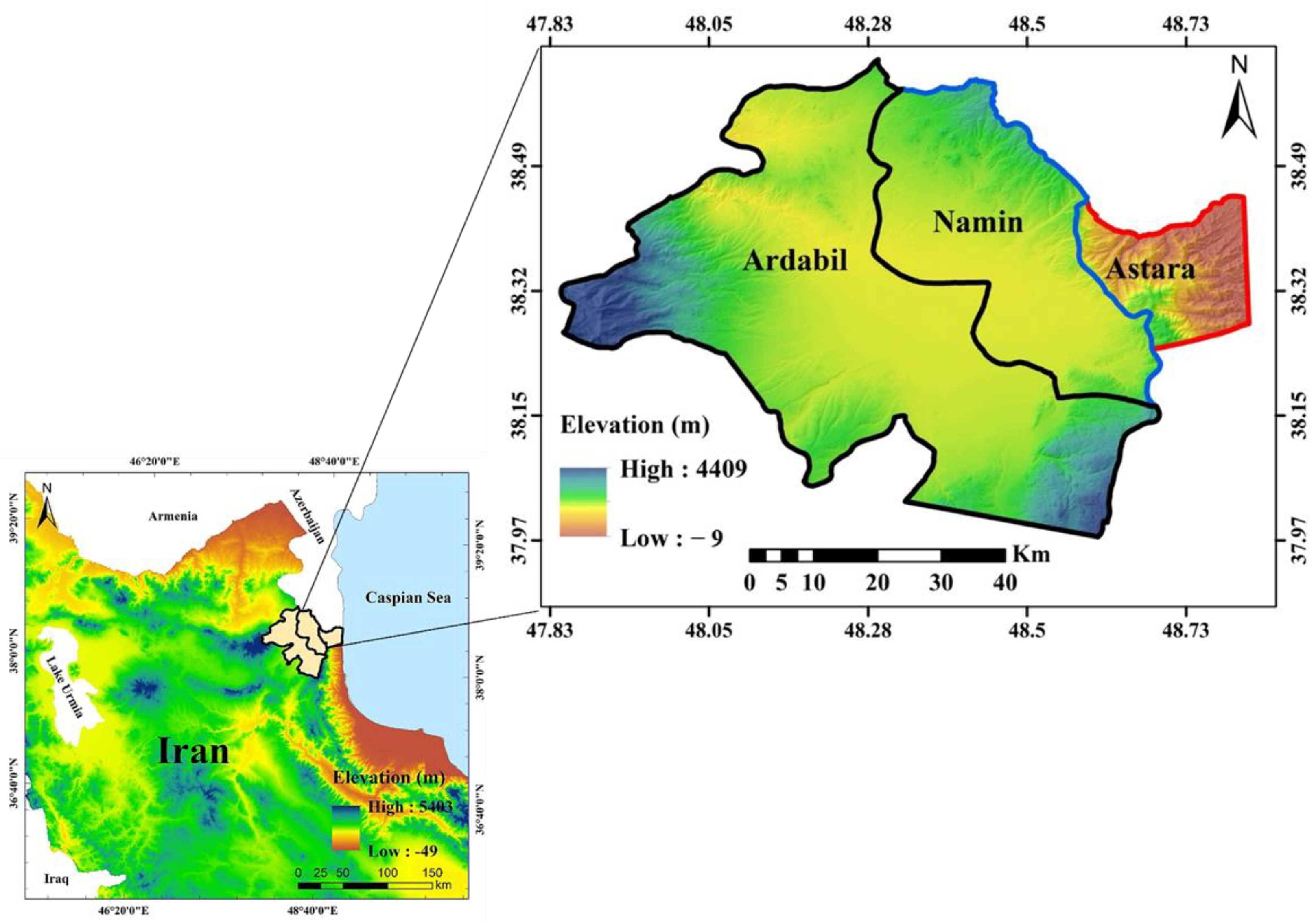
2.1. Study Area

The study area, extending between 47°48′ and 48°41’ E and 37°56′ and 38°37′ N latitude, includes the cities of Ardabil, Namin, and Astara, covers approximately 3284 km² on the western coast of the Caspian Sea, in northwest Iran (Figure 1). The meteorological and topographical features are presented in

Table 1. Main topographic and meteorological characteristics of the study area.

County	Area (km2)	Climate	Minimum Height (m)	Maximum Height (m)	Average Minimum Monthly Temperature (°C)	Average Maximum Monthly Temperature (°C)	Average Annual Rainfall (mm)
Ardabil	2017	Cold semidry	1157	4409	−8 (January)	24.6 (August)	307
Namin	945	Mediterranean	1204	2391	−6.6 (February)	25.1 (August)	378
Astara	322	Mild and humid	−9	1910	2.7 (February)	29.7 (June)	1328

across the study regions. The temperature and precipitation vary across regions (Table 1). The maximum and minimum temperatures recorded in Astara and Namin are 29.7 and −6.6 °C, respectively; Astara and Ardabil receive the maximum and minimum precipitation of 1328 and 307 mm, respectively.

2.2. Data

Sentinel 2 and Landsat 8 images were downloaded from the ESA (https://www.esa.int; accessed on 1 September 2020) USGS (www.earthexplorer.usgs.gov; 1 September 2020) websites and used to develop LULC and surface energy controlling factors (surface albedo and temperature), respectively. For the LULC map, we first collected at least 100 field samples from each given land-use class of the study area. Then, Sentinel 2 image, with a spatial resolution of 10 m from July 2019, were employed to develop a LULC map. To determine LSA and LST, the Landsat 8 images from July 2019 were used.

2.3. Image Classification

2.3.1. Preprocessing

Error adjustment is the first step in image classification, which mostly leads to accurate analysis and therefore accurate results [29,30]. Using this process, the Landsat 8 image was corrected by radiometric enhancement through Equations (1) and (2) using ENVI 5.3 software. To that end, first, Equation (1) was used to convert the digital values to spectral radiation using the calibration coefficients of the sensor [31].

Y = Gain × DN + Offset

(1)

where Y is the spectral radiation (Wm-2Ster⁻¹ μm⁻¹), DN is the pixel digital value (0 to 255), and Gain and Offset are the calibration coefficients of the sensor. Then, Equation (2) was applied to convert the spectral radiation into spectral reflection.

$$\mathsf{\rho }=\frac{{\mathsf{\pi }\mathrm{LD}}^2}{\mathrm{Esun}.\cos \left(\mathrm{SZ}\right)}$$

(2)

where $\mathsf{\rho }$ is the spectral reflection, L is the total radiation measured in the sensor, and D is the distance between the Sun and Earth at the space unit. The effects of changes in the exposure, season, latitude, and weather conditions on the images were removed by converting the spectral radiation to spectral reflectance values, which resulted in a standardized ratio that was directly applied to compare the reflections between different images and between images captured at different times. Then, the dark object subtraction (DOS) algorithm was used to ensure the quality of data and bands as well as to eliminate the atmospheric scattering effects in the Sentinel 2 image using QGIS 3.10.

2.3.2. Object-Oriented Algorithm

Segmentation and classification are the two important image classification steps using the object-oriented approach. Image segmentation into objects (homogeneous areas) can deal with the inherent error in pixel-based algorithms and therefore facilitates multiscale analysis [32]. This means that the image is first broken down into homogeneous areas and then classified, which is more effective than the pixel-based approach. Segmentation, as the fundamental step that subdivides the entire image into segments, is considered automatic feature extraction in the object-oriented procedure. The multiresolution algorithm, a bottom-up region-merging technique, was employed in this study to perform the segmentation processes.

In this study, eCognition software ver. 10.3 was used for object-oriented classification. Object-oriented classification is most commonly applied to recognize and classify LULC types. This way, various features, such as shape, texture, relationship, and layers, for each object, in terms of object attributes, were computed and properly labeled using eCognition after accurate object delineation.

2.4. LSA and LST Calculation Using the SEBAL Algorithm

The SEBAL algorithm was developed to estimate evapotranspiration, in which the LSA and LST are also calculated. The algorithm works based on the energy balance on the Earth’s surface and estimates evapotranspiration using satellite images. In this method, LSA is defined as the ratio of reflected radiation to shortwave radiation, which is calculated as follows [33].

$$\mathsf{\alpha }=\left(\frac{{\alpha }_{\mathrm{toa}}-{\alpha }_{\mathrm{path}-\mathrm{radiance}}}{{\mathsf{\tau }}_{\mathrm{sw}}^2}\right)$$

(3)

where α_path radiance is the part of incoming solar radiation across all bands that is scattered to the satellite before arriving at the Earth’s surface, and τ_sw is the transitivity of the atmosphere. The α_{path_radiance} values usually vary from 0.025 to 0.04, where f 0.03 is recommended for SEBAL according to Bastiaanssen [34]. The τ_sw is the ability of direct and diffused (scattered) radiation to transmit to the surface. This parameter value, assuming a clear sky and relatively dry conditions, was calculated based on FAO-56, as follows:

$${\tau }_{\mathrm{sw}}=0.75+2\times {10}^{-5}\times \mathrm{z}$$

(4)

where z is the average altitude above sea level in meters. It should be precisely determined in a way that is representative of the whole area’s altitude. To that end, z was the average altitude of the stations in this study. Finally, LST was estimated as follows:

$$\mathrm{LST}=\frac{{\mathrm{K}}_2}{\ln (\frac{{\epsilon }_{{\mathrm{NBK}}_1}}{{\mathrm{R}}_{\mathrm{c}}}+1)}$$

(5)

where R_c is the corrected thermal band radius, ε_NB is the surface emission of the thermal band, and K₁ and K₂ are the constants coefficients of the equation. The coefficient values for band 10 are 774.89 and 1321.08, and 480.89 and 14201 for band 11, respectively [35].

To apply image classification results in practice, their accuracy should be evaluated to ensure classification precision [36]. The error matrix is the method widely used for evaluating the accuracy of image classification [37,38]. The matrix includes the overall accuracy evaluation criteria, producer accuracy, user accuracy, and kappa coefficient, which are the most common parameters used for assessing image classification precision. Hence, one-third of the collected field samples were employed to calculate the error matrix.

3. Results

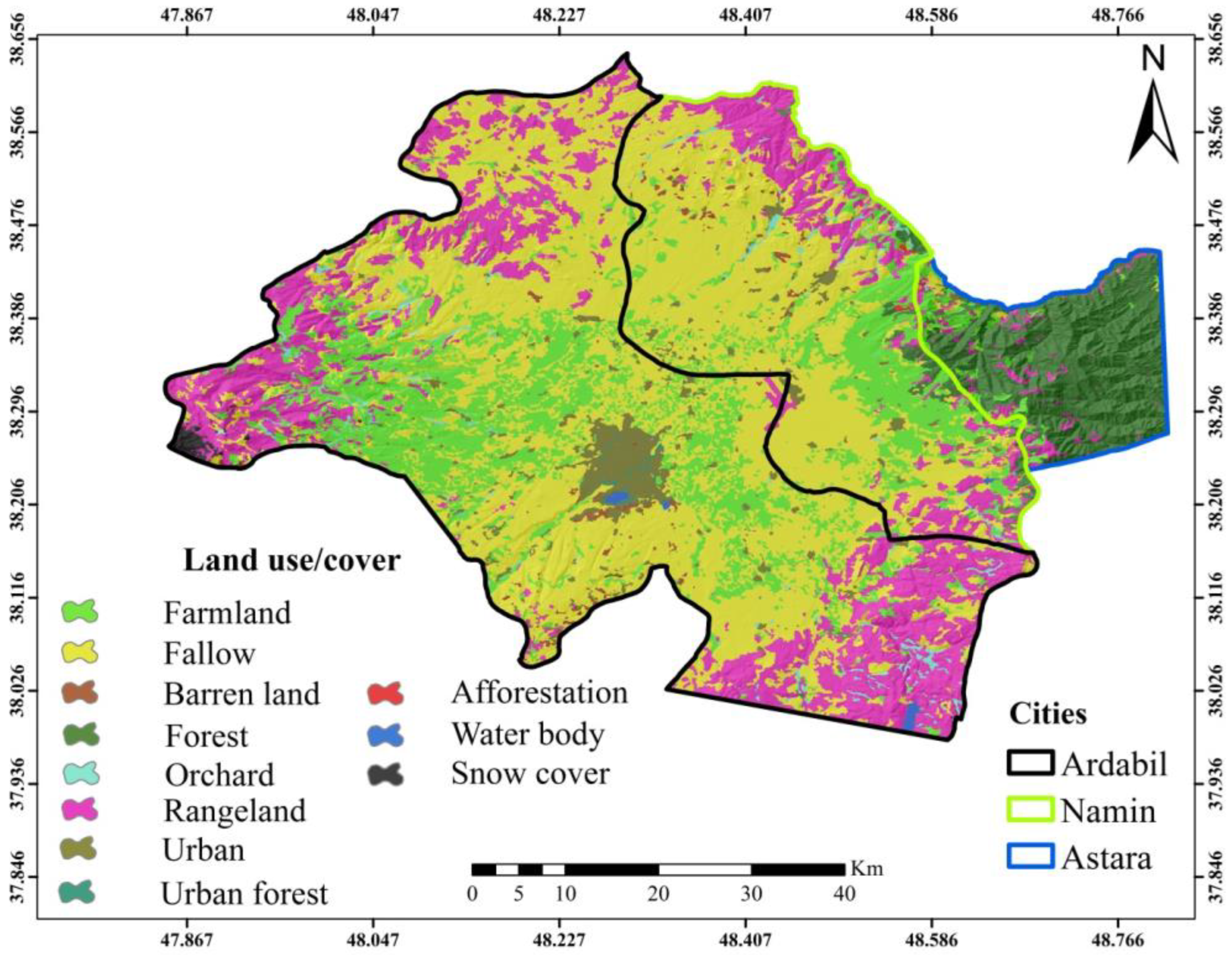
3.1. LULC Map of the Study Area

Figure 2 shows the LULC map of the study area in 2019. The results of the accuracy assessment revealed a kappa coefficient of 0.91 and overall accuracy of 0.93, which indicated the strong ability of the object-oriented algorithm to capture the LULC patterns of the region based on the field samples. In Figure 2, fallow (64,247.4 ha) and afforestation (127.7 ha) were the largest and smallest LULCs of the study area, respectively (

Table 2. LULC types and their covered area across the study area.

LULC	Description	Area
		ha	%
Fallow	Agricultural land that was not planted during imaging.	153,809	45.57
Rangeland	Uncultivated shrub lands, grasslands, and woodlands suitable for grazing and wild animals.	69,940.4	20.72
Farmland	Lands with crops at the time of imaging.	64,247.4	19.03
Forest	Naturally dominated by different trees species.	28,981.9	8.59
Urban	Humanmade infrastructure, such as houses, factories, and asphalt roads, that have caused the impenetrability of the land surface.	11,832.6	3.5
Orchard	Land devoted to the cultivation of fruit and nut trees or shrubs that is maintained for food production.	4352.25	1.29
Barren land	Land where no traces of human manipulation can be found, and its vegetation/pasture is very weak, so the land is not in a productive or active state.	2156	0.64
Snow cover	A layer of snow that covers ground surface.	989.875	0.29
Water body	Areas completely covered by water, such as lakes, reservoirs, rivers, streams, and ponds.	563.875	0.17
Urban forest	Urban forests include trees and shrubs in yards, along streets and utility corridors, in protected areas, and in watersheds. These include individual trees, street trees, and green spaces with trees, along with the vegetation and soil beneath them.	535.688	0.16
Afforestation lands	Areas with newly established forests through planting or seedlings.	127.688	0.04
Total	All land uses/covers across the study area.	337,536.7	100

).

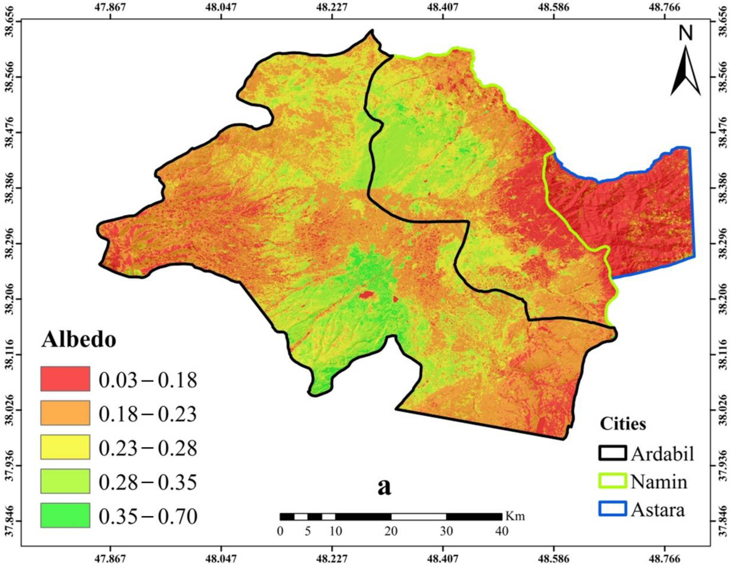
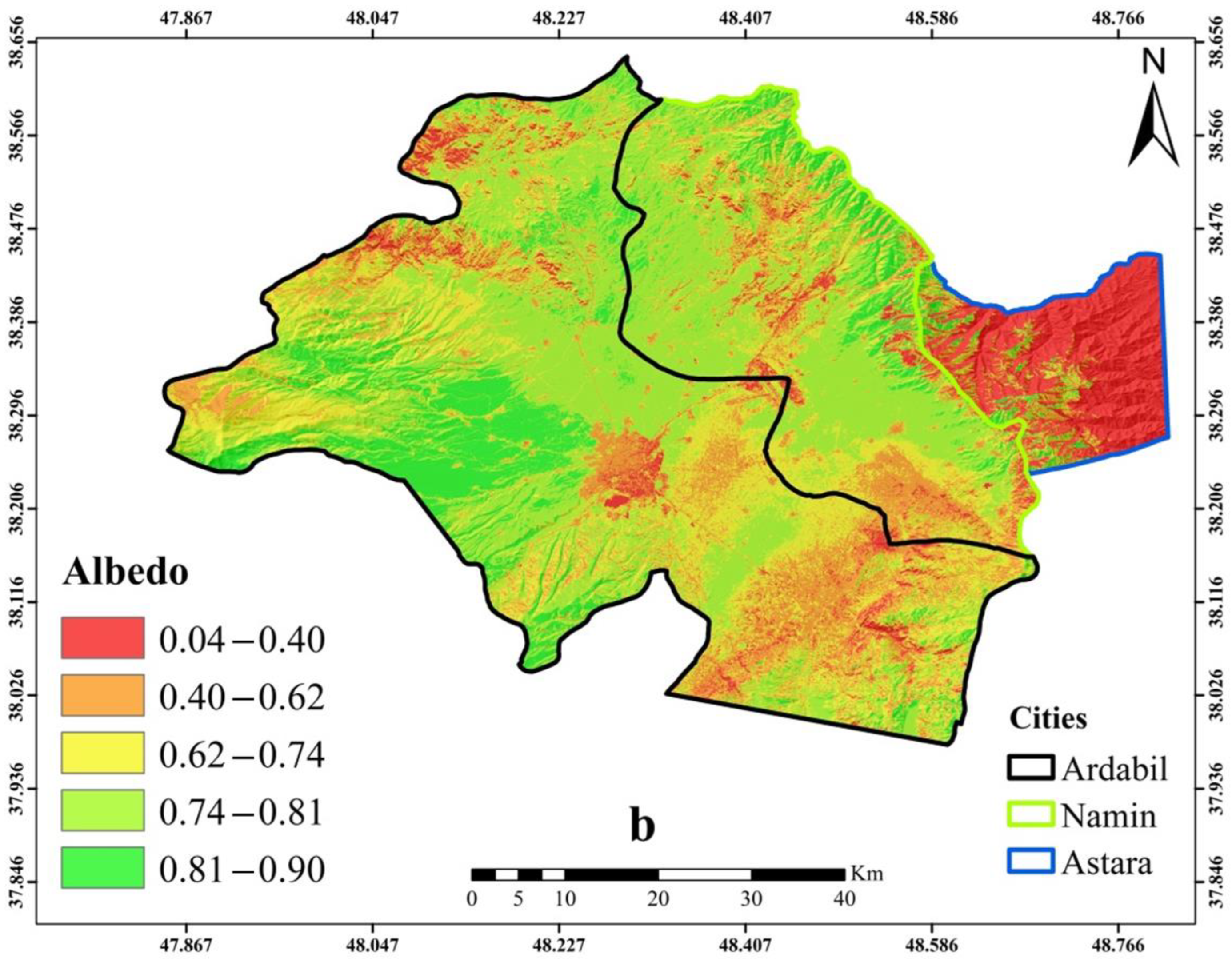
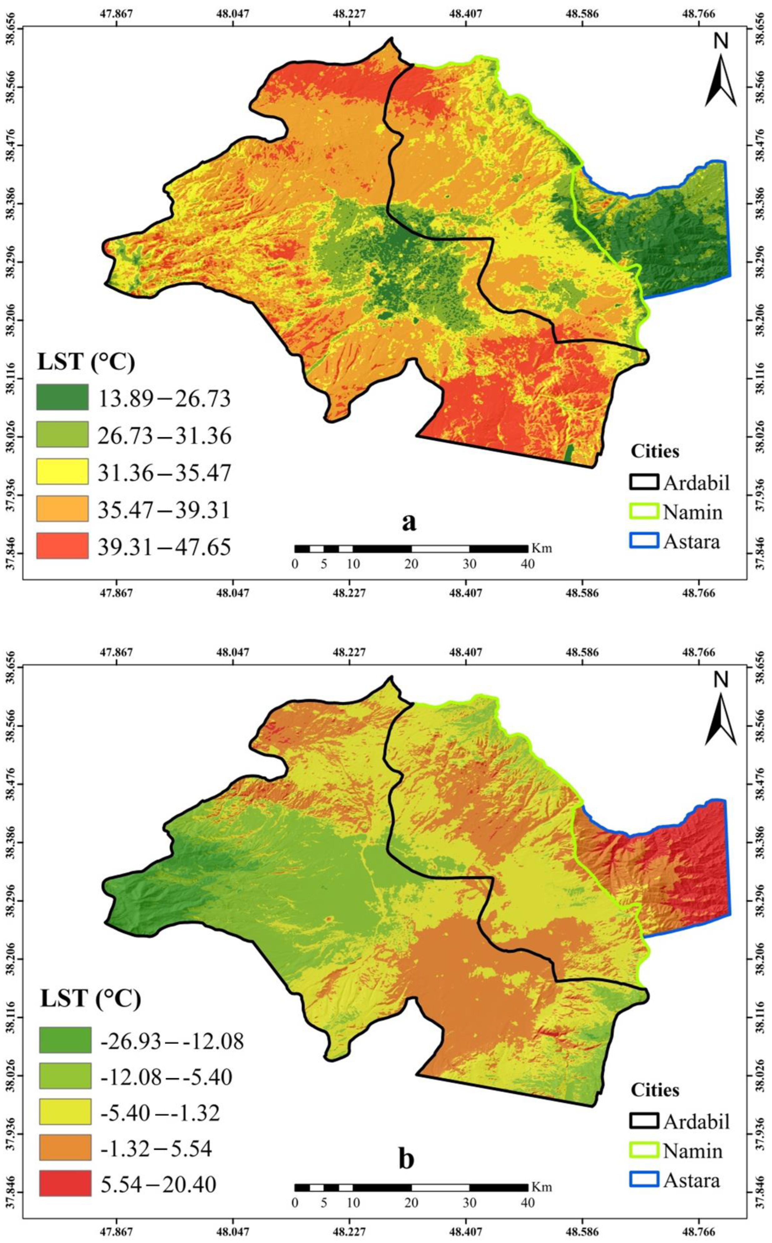
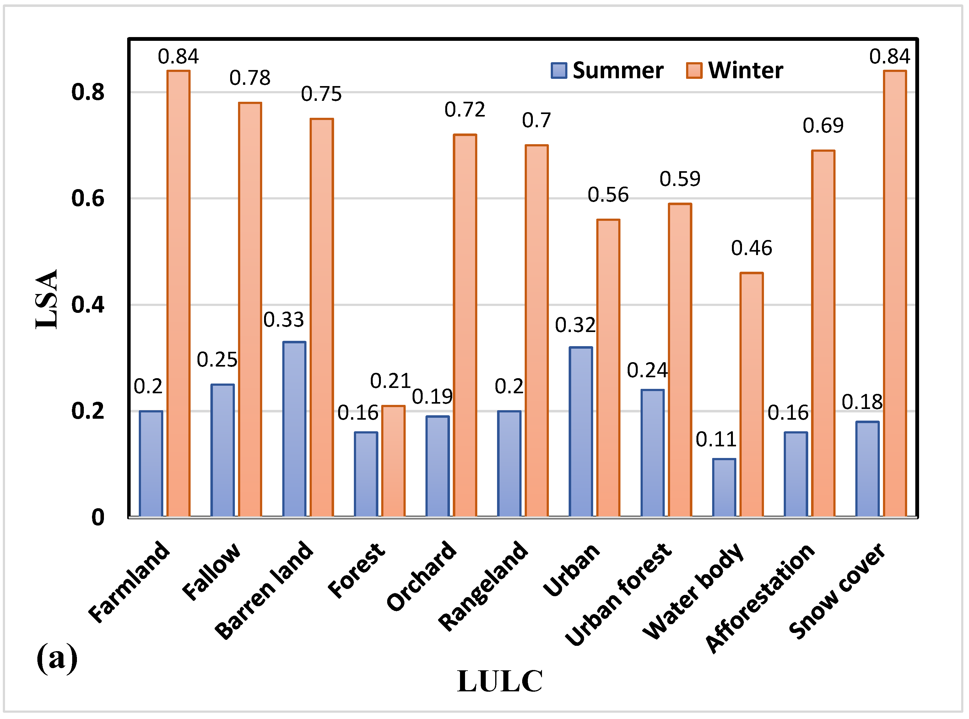
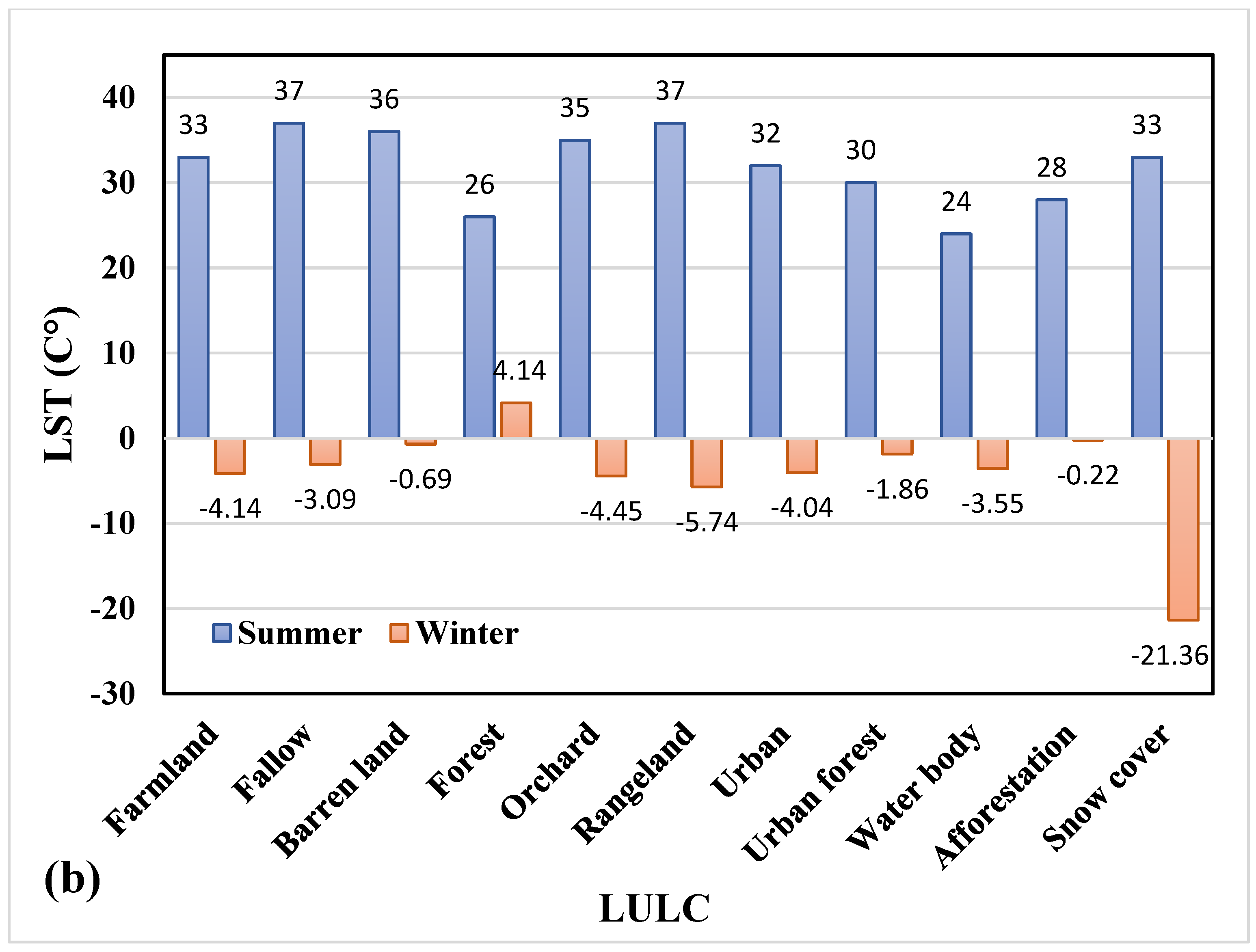
3.2. LSA and LST across the Study Area

Figure 3 shows the LSA maps of the study area for the summer and winter seasons. It is evident that LSA values were high during winter compared with during the summer. Hence, the values of 0.04–0.90 and 0.03–0.70 were estimated during winter and summer, respectively. According to the LSA map (Figure 3a), the low values (0.03–0.28) in summer mostly came from the LULCs that covered the majority of the region. In winter (Figure 3b), the high values (0.62–0.90) were from the LULCs that covered a substantial area in the region.

Figure 4 depicts the developed maps for LSA in summer and winter. According to this figure, the maximum and minimum temperatures of 47.65 °C and −26.93 °C were estimated for the region in summer and winter, respectively.

Table 3. LULC contribution in LST (°C) and LSA.

LULC	Summer		Winter
	LST	LSA	LST	LSA
Farmland	33	0.2	−4.14	0.84
Fallow	37	0.25	−3.09	0.78
Barren land	36	0.33	−0.69	0.75
Forest	26	0.16	4.14	0.21
Orchard	35	0.19	−4.45	0.72
Rangeland	37	0.2	−5.74	0.70
Urban	32	0.32	−4.4	0.56
Urban forest	30	0.24	−1.86	0.59
Water body	24	0.11	−3.55	0.46
Afforestation	28	0.16	−0.22	0.69
Snow cover	33	0.18	−21.36	0.84

presents the values for LSA and LSA, individually, across the different LULCs in two study periods. According to this table, the maximum and minimum values of LSA were associated with farmland (0.84) and water bodies (0.11), respectively.

Additionally, the maximum value of LSA was simultaneously attributed to fallow and rangeland, while its minimum value was attained from snow-covered land. The graphs were established to better understand and compare the two climate-affecting factors in the studied period (Figure 5).

4. Discussion and Conclusions

To assessing the effect of different LULCs on LSA and LST changes, we tested a hypothesis that forests are always as effective at mitigating global warming as we expect. Remote sensing measurements were applied to detect LSA and LST because different surface substances naturally have their own specific albedo across different scales. We applied Landsat 8 images with a spatial resolution of 30 m to estimate LSA and LST. Additionally, Sentinel 2 images with a resolution of 10 m were employed to develop the LULC map. LSA and LST were estimated using the SEBAL algorithm and Landsat images. Our results regarding image classification indicated the high accuracy of the object-oriented algorithm in capturing LULC changes, in accordance with the findings of Whiteside et al. [39]. Based on the results, the maximum and minimum LAS were attributed to farmland and water bodies, respectively, in line with the results reported by Asadi et al. [33] and Münch et al. [40], who revealed the contribution of residential areas to LAS changes across the different LULCs. This difference might occur due to the type of materials used on ceilings, walls, and facades, which may be constructed with high-reflectivity materials [41]. On the contrary, farmland and forests showed the maximum and minimum contributions to LSA in winter, respectively. Azizah et al. [42] investigated the effect of LULC change on NDVI, LAS, and heat fluxes, and concluded that the distribution of LSA for each LULC class from the lowest to the highest was forest, plantation, cropland, shrubs, and settlements. The distribution of NDVI was the opposite to that of LSA. According to the results of image classification, it is expected that the impact of residential areas and forests, with the maximum contribution to LAS, on regional warming will be higher than that of barren land because of their widespread area.

Trees seem to be one of the most popular options when it comes to tackling global warming in countries that have made little progress in controlling carbon dioxide emissions. Hence, many governments have developed cutting-edge plans in order to plant a large number of trees to absorb carbon dioxide from the atmosphere to help reduce the effects climate change. However, a newly emerged view suggests that trees may not always be as helpful to fighting global warming as the general public thinks, because the dark leaves of trees can increase the temperature by absorbing sunlight, which results in the elimination of the forests’ cooling effects [43]. Our findings imply the low contribution of forests to LSA (summer: 0.16 and winter: 0.21), which is in agreement with the findings of Asadi et al. [33], who assessed the contribution of different LULCs on LSA using SEBAL and metric methods in Ardabil, and concluded that forests followed by water bodies contributed the least to the LSA. Additionally, our results are in line with those of Yan et al. [44], who examined LSA variations between 2002 to 2019 during a period of forest area growth in China, and concluded that the albedo was increased by increased forest greening (increased bright canopy) and decreased dark crevices. They also found that range greening reduced the LSA during the same growing period. Therefore, the contribution of different LULC classes to LSA can vary based on topographic and geographical features.

Our results demonstrated the capability of the SEBAL algorithm to capture LST because this algorithm estimates the evapotranspiration using a minimum amount of in situ data at instantaneous, daily, and seasonally scales using an energy balance process at the pixel level. Our results support the previous finding that SEBAL is efficient in measuring evapotranspiration and other LST fluxes [45].

According to the results, the maximum and minimum LST values in summer were obtained from fallow land associated with rangeland and water bodies, respectively. In winter, forests and snow cover showed the highest and lowest LST, respectively. This finding is in accordance with that of Nadizadeh Shourabeh et al. [46], who indicated a high average temperature of fallow land during 1992–2015. Additionally, we obtained the minimum LST from water bodies, which is in line with the findings of Feizizadeh et al. [47]. These results can be attributed to the nonuniformity of fallow land, which is a combination of grass, plants, and soil surface that causes the largest temperature variation on the ground [46]. Merga et al. [48] investigated the LST changes in response to LULC dynamics in the Didsa River sub-basin in western Ethiopia, and showed that the highest LST values were on bare land, settlement areas, and farmland, whereas forests and water bodies had the lowest LST. It should be kept in mind that all these results should be interpreted in light of biophysical factors (e.g., solar radiation intensity, surface moisture, wind speed, and humidity), which may not have been stable or stationary during the timeframes when the data were collected [49].

Overall, our findings demonstrated that forests do not always have a climate-modifying role and may not serve as a driver of regional or global warming. However, this finding might be due to the geographical location or limited forest area in this study. Because forests, in almost all previous studies, have played a decisive role in global climate, our findings provide insight into the role of forest areas in global warming and climate change, which can be considered as a new insight in this field. However, further research concerning the role of forest areas in global warming is required to draw a general conclusion about the local, regional, and global cooling or warming effects of forests.

References

1. Houghton, R. Aboveground forest biomass and the global carbon balance. Glob. Change Biol. 2005, 11, 945–958. [Google Scholar] [CrossRef]
2. Zhang, K.; Ali, A.; Antonarakis, A.; Moghaddam, M.; Saatchi, S.; Tabatabaeenejad, A.; Chen, R.; Jaruwatanadilok, S.; Cuenca, R.; Crow, W.T. The sensitivity of North American terrestrial carbon fluxes to spatial and temporal variation in soil moisture: An analysis using radar-derived estimates of root-zone soil moisture. J. Geophys. Res. Biogeosci. 2019, 124, 3208–3231. [Google Scholar] [CrossRef]
3. Li, X.; Jin, H.; Sun, L.; Wang, H.; He, R.; Huang, Y.; Chang, X. Climate warming over 1961–2019 and impacts on permafrost zonation in Northeast China. J. For. Res. 2022, 33, 767–788. [Google Scholar] [CrossRef]
4. Mafi-Gholami, D.; Zenner, E.K.; Jaafari, A.; Bakhtiari, H.R.; Tien Bui, D. Multi-hazards vulnerability assessment of southern coasts of Iran. J. Environ. Manag. 2019, 252, 109628. [Google Scholar] [CrossRef]
5. Chen, Z.; Liu, Z.; Yin, L.; Zheng, W. Statistical analysis of regional air temperature characteristics before and after dam construction. Urban Clim. 2022, 41, 101085. [Google Scholar] [CrossRef]
6. Wang, G.; Zhao, B.; Lan, R.; Liu, D.; Wu, B.; Li, Y.; Li, Q.; Zhou, H.; Liu, M.; Liu, W. Experimental study on failure model of tailing dam overtopping under heavy rainfall. Lithosphere 2022, 2022, 5922501. [Google Scholar] [CrossRef]
7. Xu, L.; Liu, X.; Tong, D.; Liu, Z.; Yin, L.; Zheng, W. Forecasting urban land use change based on cellular automata and the PLUS model. Land 2022, 11, 652. [Google Scholar] [CrossRef]
8. Yin, L.; Wang, L.; Zheng, W.; Ge, L.; Tian, J.; Liu, Y.; Yang, B.; Liu, S. Evaluation of empirical atmospheric models using Swarm-C satellite data. Atmosphere 2022, 13, 294. [Google Scholar] [CrossRef]
9. Adnan, R.M.I.; Dai, H.-L.; Ewees, A.A.; Shiri, J.; Kisi, O.; Zounemat-Kermani, M. Application of improved version of multi verse optimizer algorithm for modeling solar radiation. Energy Rep. 2022, 8, 12063–12080. [Google Scholar]
10. Kim, Y.; Kimball, J.S.; Zhang, K.; Didan, K.; Velicogna, I.; McDonald, K.C. Attribution of divergent northern vegetation growth responses to lengthening non-frozen seasons using satellite optical-NIR and microwave remote sensing. Int. J. Remote Sens. 2014, 35, 3700–3721. [Google Scholar] [CrossRef] [Green Version]
11. Yang, J.; Shuai, Y.; Duan, J.; Xie, D.; Zhang, Q.; Zhao, R. Impact of BRDF spatiotemporal smoothing on land surface albedo estimation. Remote Sens. 2022, 14, 2001. [Google Scholar] [CrossRef]
12. Liu, Y.; Zhang, K.; Li, Z.; Liu, Z.; Wang, J.; Huang, P. A hybrid runoff generation modelling framework based on spatial combination of three runoff generation schemes for semi-humid and semi-arid watersheds. J. Hydrol. 2020, 590, 125440. [Google Scholar] [CrossRef]
13. Klein, R.J.; Midglev, G.; Preston, B.; Alam, M.; Berkhout, F.; Dow, K.; Shaw, M. Climate Change 2014: Impacts, Adaptation, and Vulnerability; IPCC Fifth Assessment Report; Cambridge University Press: Cambridge, UK; New York, NY, USA, 2014. [Google Scholar]
14. Lenton, T.M.; Vaughan, N.E. The radiative forcing potential of different climate geoengineering options. Atmos. Chem. Phys. 2009, 9, 5539–5561. [Google Scholar] [CrossRef] [Green Version]
15. Robock, A.; Marquardt, A.; Kravitz, B.; Stenchikov, G. Benefits, risks, and costs of stratospheric geoengineering. Geophys. Res. Lett. 2009, 36, L19703. [Google Scholar] [CrossRef] [Green Version]
16. Jacobson, M.Z.; Ten Hoeve, J.E. Effects of urban surfaces and white roofs on global and regional climate. J. Clim. 2012, 25, 1028–1044. [Google Scholar] [CrossRef]
17. Betts, R.A. Offset of the potential carbon sink from boreal forestation by decreases in surface albedo. Nature 2000, 408, 187–190. [Google Scholar] [CrossRef] [PubMed]
18. Carrer, D.; Pique, G.; Ferlicoq, M.; Ceamanos, X.; Ceschia, E. What is the potential of cropland albedo management in the fight against global warming? A case study based on the use of cover crops. Environ. Res. Lett. 2018, 13, 044030. [Google Scholar] [CrossRef] [Green Version]
19. Zhao, T.; Shi, J.; Lv, L.; Xu, H.; Chen, D.; Cui, Q.; Jackson, T.J.; Yan, G.; Jia, L.; Chen, L. Soil moisture experiment in the Luan River supporting new satellite mission opportunities. Remote Sens. Environ. 2020, 240, 111680. [Google Scholar] [CrossRef]
20. Zhang, Y.; Sharma, S.; Bista, M.; Li, M. Characterizing changes in land cover and forest fragmentation from multitemporal Landsat observations (1993–2018) in the Dhorpatan Hunting Reserve, Nepal. J. For. Res. 2022, 33, 159–170. [Google Scholar] [CrossRef]
21. Zhao, T.; Shi, J.; Entekhabi, D.; Jackson, T.J.; Hu, L.; Peng, Z.; Yao, P.; Li, S.; Kang, C.S. Retrievals of soil moisture and vegetation optical depth using a multi-channel collaborative algorithm. Remote Sens. Environ. 2021, 257, 112321. [Google Scholar] [CrossRef]
22. Kumari, P.; Kapur, S.; Garg, V.; Kumar, K. Effect of surface temperature on energy consumption in a calibrated building: A case study of Delhi. Climate 2020, 8, 71. [Google Scholar] [CrossRef]
23. Sekertekin, A.; Bonafoni, S. Land surface temperature retrieval from Landsat 5, 7, and 8 over rural areas: Assessment of different retrieval algorithms and emissivity models and toolbox implementation. Remote Sens. 2020, 12, 294. [Google Scholar] [CrossRef] [Green Version]
24. Zhou, G.; Yang, F.; Xiao, J. Study on pixel entanglement theory for imagery classification. IEEE Trans. Geosci. Remote Sens. 2022, 60, 5409518. [Google Scholar] [CrossRef]
25. Zhou, G.; Deng, R.; Zhou, X.; Long, S.; Li, W.; Lin, G.; Li, X. Gaussian inflection point selection for LiDAR hidden echo signal decomposition. IEEE Geosci. Remote Sens. Lett. 2021, 19, 6502705. [Google Scholar] [CrossRef]
26. Dash, P.; Göttsche, F.-M.; Olesen, F.-S.; Fischer, H. Retrieval of land surface temperature and emissivity from satellite data: Physics, theoretical limitations and current methods. J. Indian Soc. Remote Sens. 2001, 29, 23–30. [Google Scholar] [CrossRef]
27. Ghent, D.; Veal, K.; Trent, T.; Dodd, E.; Sembhi, H.; Remedios, J. A new approach to defining uncertainties for MODIS land surface temperature. Remote Sens. 2019, 11, 1021. [Google Scholar] [CrossRef] [Green Version]
28. Zhao, F.; Song, L.; Peng, Z.; Yang, J.; Luan, G.; Chu, C.; Ding, J.; Feng, S.; Jing, Y.; Xie, Z. Night-time light remote sensing mapping: Construction and analysis of ethnic minority development index. Remote Sens. 2021, 13, 2129. [Google Scholar] [CrossRef]
29. Tian, H.; Huang, N.; Niu, Z.; Qin, Y.; Pei, J.; Wang, J. Mapping winter crops in China with multi-source satellite imagery and phenology-based algorithm. Remote Sens. 2019, 11, 820. [Google Scholar] [CrossRef] [Green Version]
30. Li, Q.; Song, D.; Yuan, C.; Nie, W. An image recognition method for the deformation area of open-pit rock slopes under variable rainfall. Measurement 2022, 188, 110544. [Google Scholar] [CrossRef]
31. Lillesand, T.; Kiefer, R.W.; Chipman, J. Remote Sensing and Image Interpretation; John Wiley & Sons: New York, NY, USA, 2015. [Google Scholar]
32. Blaschke, T. Object based image analysis for remote sensing. ISPRS J. Photogramm. Remote Sens. 2010, 65, 2–16. [Google Scholar] [CrossRef] [Green Version]
33. Asadi, M.; Kamran, K.V. Comparison of SEBAL, METRIC, and ALARM algorithms for estimating actual evapotranspiration of wheat crop. Theor. Appl. Climatol. 2022, 149, 327–337. [Google Scholar] [CrossRef]
34. Bastiaanssen, W.G. SEBAL-based sensible and latent heat fluxes in the irrigated Gediz Basin, Turkey. J. Hydrol. 2000, 229, 87–100. [Google Scholar] [CrossRef]
35. Ghaleb, F.; Mario, M.; Sandra, A.N. Regional landsat-based drought monitoring from 1982 to 2014. Climate 2015, 3, 563–577. [Google Scholar] [CrossRef] [Green Version]
36. Aitkenhead, M.; Aalders, I. Classification of landsat thematic mapper imagery for land cover using neural networks. Int. J. Remote Sens. 2008, 29, 2075–2084. [Google Scholar] [CrossRef]
37. Wang, G.; Zhao, B.; Wu, B.; Zhang, C.; Liu, W. Intelligent prediction of slope stability based on visual exploratory data analysis of 77 in situ cases. Int. J. Min. Sci. Technol. 2022, in press. [Google Scholar] [CrossRef]
38. Adnan, R.M.I.; Ewees, A.A.; Parmar, K.S.; Yaseen, Z.M.; Shahid, S.; Kisi, O. The viability of extended marine predators algorithm-based artificial neural networks for streamflow prediction. Appl. Soft Comput. 2022, 131, 109739. [Google Scholar]
39. Whiteside, T.G.; Boggs, G.S.; Maier, S.W. Comparing object-based and pixel-based classifications for mapping savannas. Int. J. Appl. Earth Obs. Geoinf. 2011, 13, 884–893. [Google Scholar] [CrossRef]
40. Münch, Z.; Gibson, L.; Palmer, A. Monitoring effects of land cover change on biophysical drivers in rangelands using albedo. Land 2019, 8, 33. [Google Scholar] [CrossRef] [Green Version]
41. Akbari, H.; Kolokotsa, D. Three decades of urban heat islands and mitigation technologies research. Energy Build. 2016, 133, 834–842. [Google Scholar] [CrossRef]
42. Azizah, S.N.N.; June, T.; Salmayenti, R.; Ma’rufah, U.; Koesmaryono, Y. Land use change impact on normalized difference vegetation index, surface albedo, and heat fluxes in Jambi province: Implications to rainfall. Agromet 2022, 36, 51–59. [Google Scholar] [CrossRef]
43. Popkin, G. How much can forests fight climate change? Nature 2019, 565, 280–283. [Google Scholar] [CrossRef] [PubMed] [Green Version]
44. Yan, H.; Wang, S.; Dai, J.; Wang, J.; Chen, J.; Shugart, H.H. Forest greening increases land surface albedo during the main growing period between 2002 and 2019 in China. J. Geophys. Res. Atmos. 2021, 126, e2020JD033582. [Google Scholar] [CrossRef]
45. Ebrahimi, H.; Gandomkar, A.; Almodarresi, A.; Ramesht, M.H. Estimation of land surface temperature and vegetation effects on surface temperature by using bands of MODIS images (case study: Toysercan basin). Geogr. Reg. Plan. 2016, 6, 23–32. [Google Scholar]
46. Nadizadeh, S.S.; Hamzeh, S.; Kiavarz, M. Investigating spatial and temporal land use changes and urban development and its effect on the increase of land surface temperature using Landsat multi-temporal images (case study: Gorgan city). Geogr. Urban Plan. Res. GUPR 2018, 6, 545–568. [Google Scholar]
47. Feizizadeh, B.; Blaschke, T. Thermal remote sensing for land surface temperature monitoring: Maraqeh County, Iran. In Proceedings of the 2012 IEEE International Geoscience and Remote Sensing Symposium, Munich, Germany, 22–27 July 2012; pp. 2217–2220. [Google Scholar]
48. Merga, B.B.; Moisa, M.B.; Negash, D.A.; Ahmed, Z.; Gemeda, D.O. Land surface temperature variation in response to land-use and land-cover dynamics: A case of Didessa River sub-basin in Western Ethiopia. Earth Syst. Environ. 2022, 6, 803–815. [Google Scholar] [CrossRef]
49. Dissanayake, D.; Morimoto, T.; Ranagalage, M.; Murayama, Y. Land-use/land-cover changes and their impact on surface urban heat islands: Case study of Kandy City, Sri Lanka. Climate 2019, 7, 99. [Google Scholar] [CrossRef]
Figure 1. Map of the study area location.
Sustainability 14 16963 g001
Figure 2. LULC map of study area produced using the objected-oriented algorithm applied to Sentinel 2 images.
Sustainability 14 16963 g002
Figure 3. Supervised classification results for 30 m LSA in (a) summer and (b) winter produced using the SEBAL algorithm.
Sustainability 14 16963 g003aSustainability 14 16963 g003b
Figure 4. Supervised classification results for 30 m LST in (a) summer and (b) winter.
Sustainability 14 16963 g004
Figure 5. Contribution of different LULC classes to (a) LSA and (b) LST in the study period.
Sustainability 14 16963 g005aSustainability 14 16963 g005b