
Analysis of Bed Sorting Methods for One Dimensional Sediment Transport Model
1
Department of Civil and Environmental Engineering, Incheon National University, 119 Academy-ro, Yeonsu-gu, Incheon 22012, Republic of Korea
2
Incheon Disaster Prevention Research Center, Incheon National University, 119 Academy-ro, Yeonsu-gu, Incheon 22012, Republic of Korea
*
Author to whom correspondence should be addressed.
Sustainability 2023, 15(3), 2269; https://0-doi-org.brum.beds.ac.uk/10.3390/su15032269
Submission received: 29 November 2022
/
Revised: 14 January 2023
/
Accepted: 19 January 2023
/
Published: 26 January 2023
(This article belongs to the Collection Modeling and Simulations for Sustainable Water Environments)
Abstract
:Proper estimation of sediment movement is very critical for the management of alluvial rivers. Computing the sediment transport with single particle size is possible. However, particles on the river bed and in transport have a size distribution. It is very important to estimate bed material size change, such as bed armoring, in case of scour. In this study, the applicability of the bed sorting method, which is available with HEC-RAS, was analyzed. Bed sorting methods divide the bed into two or three layers. Numerical simulations were conducted in the Geum River, Korea. The performance of the simulation with respect to bed sorting methods was evaluated by considering the temporal change of bed material size during the scour and armoring process. Three layer methods are not applicable for a natural river and had oscillatory temporal bed material size variation. The two layer method has stable temporal bed material size changes and predicts the armoring of the bed properly even with limited field data. Consequently, the active layer method is reliable for natural rivers to simulate the bed material size change while applications of three layer methods require sufficient investigation.
1. Introduction
The fluvial process is a dominant factor in the shape of a river. The change of topography affects the hydraulics of the river. Furthermore, the safety and the functional performance of hydraulic structures are affected by the change of topography. Sedimentation causes floods by reducing reservoir capacity and reducing flow area [1]. Flood level rise and water storage capacity reductions in reservoirs due to sedimentation should be solved. Scour dominant cases cause bridge failures [2,3]. Many cases of bridges failure due to excessive scour induced by flood have been reported [4,5]. Scour caused 60% of the destruction of more than 1000 piers in the United States over a period of 30 years [2,6]. Numerous European bridges were damaged due to scour as well [7]. Similarly, bridge failures were observed in South America and Asia [8,9,10,11]. Therefore, it is necessary to estimate the amount of sediment erosion and deposition properly to respond to the sediment problems.
Numerous studies were conducted to understand the behavior of sediment particles. Ahn and Yang (2015) suggested a method for determining the recovery factor for the simulation of non-equilibrium sedimentation to reflect the spatial and temporal delay of sediment particle movement. The applicability was verified by comparing the simulation results with previous studies [12]. The flow instability during a flood affects the structures and particle behaviors. Previous studies demonstrated that the analysis of sediment particle behavior is important for an unsteady state by showing that the sediment transport can vary depending on flow conditions [13].
There are empirical and analytical methods for analyzing the sediment transport in rivers. The empirical method analyzes the relationship between hydraulic characteristics and sediment behavior with physical experiments or field measurements. The results of the empirical analysis are reliable because they are realistic. However, it has disadvantages. It takes significant effort to collect the data and has a distortion or scale effect when the physical model is used [14].
The analytical method obtains mathematical solutions using the governing equations of flow and sediment transport. Numerous models were developed for sediment transport analysis. HEC-6, developed by the U.S. Army Corps of Engineers (USACE), is one of the most famous numerical models that can simulate river bed change [15]. The analytical method is commonly used for sediment transport analysis because it can reduce the effort for model construction and has no distortion effect on the model. In general, a three dimensional model and a one dimensional model are used separately according to the spatial extent of the basin and simulation time duration [16].
Various approaches have been suggested to estimate sediment quantities. Guo et al. (2020) investigated the relationship between the inflow sediment concentration and the outflow amount of sediment with respect to the magnitude of the flood, using the observed flow rate and sediment load data to understand sediment transport characteristics of the Lower Yellow River. As a result, sediment concentrations for deposition, erosion, and equilibrium were determined according to the magnitude of the flood at the Xiaolangdi station [17]. Wang et al. (2007) studied the alluvial processes at several cross sections of the Yellow River and one of its tributaries, the Weihe River, after the construction of the Sanmenxia Dam. As a result of analyzing the observed data from the river bed, it was noted that the flood level increased and the reservoir capacity decreased due to the deposition in the upstream part of the reservoir. Furthermore, at the downstream part, the stability of the dyke reduced due to the lateral migration of the channel in the future [18]. Ahn et al. (2013) evaluated the flushing efficiency according to the operation of the dam spillway gate in order to manage storage capacity reduction due to sedimentation. Flushing with the gate operation scenarios was simulated and the flushing efficiency was evaluated [1]. Kwon et al. (2008) simulated a long-term river bed change of the Gokreung Stream using the HEC-6 model to analyze the effect of the removal of weirs on the river bed. After the weirs were removed, the change in the amount of sediment transport over time and the pattern of bed elevation change were confirmed. The time to reach the equilibrium bed of the Gokreung Stream was predicted [15]. Kiat et al. (2008) simulated the change of the Kulim River bed with respect to the sediment transport formula and the roughness coefficient. They noted that the basin characteristics that change after urbanization can affect the sediment transport and river bed elevation [19].
HEC-RAS, developed in the 1970s by the USACE, is a representative numerical model that can compute water surface curves and sediment transport. HEC-RAS is commonly used for numerical investigation of water surface and flow velocity with the construction of bridges [20]. In addition, it has the capacity of urban flood simulation due to the backwater of reach [21]. The computation of sediment transport is analyzed by a sediment continuity equation, the Exner equation [22]. It is necessary to compute the amount of sediment that flows out of the control volume to analyze the sediment continuity equation. However, it is very difficult to figure out a solution for sediment transport, because the relationship between sediment and hydraulic properties is very complicated. Flow characteristics are the dominant factor for the sediment transport. Flow characteristics are very complicated and change continuously due to the effects of turbulence, vertical flow velocity distribution, and many other aspects. The complexity and continuous variation of flow characteristics make the analysis of the sediment transport very difficult. Therefore, various approaches have tried to improve the accuracy of the sediment transport computation.
HEC-RAS was updated consistently to improve the performance of the model. Brunner and Gibson (2005) explained the improvements of functions related to sediment transport. In order to confirm the performance of the updated HEC-RAS, previous laboratory data and simulation results were compared [23]. Gibson and Piper (2007) compared and analyzed the sensitivity and applicability of the bed mixing algorithm options available with HEC-RAS [24]. Gibson et al. (2017) introduced additional functions and features of the upgraded version of the HEC-RAS model. Sediment transport modeling for unsteady flow and the Copeland method for the bed sorting were added to this version [25].
In general, the scour process occurs from the upper part of the river bed. The HEC-RAS model divides the river bed into an active layer and an inactive layer during the process of computation of sediment transport. The active layer is where the sediment transport occurs, and there is no movement of sediment particles in the inactive layer. Armoring affects the sediment transport on the river bed. The armoring of the river bed reduces the amount of erosion. The finer bed materials are transported first and then the coarser materials are placed on the river bed surface [26]. In order to apply the effect of armoring to the computation of sediment transport, three methods: the active layer, Thomas, and Copeland bed sorting methods, are available with HEC-RAS. The Thomas and Copeland methods divide the active layer into a cover layer and a subsurface layer. Both methods have three bed layers and reflect the effect of armoring in the computation of the sediment transport. Active layer methods divide the bed layer into two layers only: active and inactive layers. Since the armoring is an important factor which reduces erosion from the bed, the application of a proper method is essential for the computation of sediment transport [23,25]. Therefore, the applicability of the two bed sorting methods according to the bed conditions was evaluated to suggest a proper way to select a bed sorting method.
2. Methodology
2.1. HEC-RAS Sediment Transport Modeling
Sediment transport is computed with the sediment continuity equation, the Exner equation, as shown in Equation (1).
where B is channel width, Z0 is bed elevation, λp is the porosity of the active layer, t is time, x is length, and Qs is sediment discharge.
The porosity of the active layer is required to convert the mass change into volume. HEC-RAS calculates the change of bed thickness with time using the deviation of the inflow and outflow of sediment in the control volume, which is the right hand side of Equation (1) [22,27]. It is necessary to calculate the amount of sediment flowing out of the control volume. However, the process of finding a solution for the relationship between hydraulics and sediment characteristics is very complicated. HEC-RAS calculates the sediment transport capacity, which is the transportable mass for each grain size of the active layer. The deposition and the erosion amounts are determined for each grain size class by comparing the calculated sediment transport potential and the amount of inflow sediment from the upstream. If the inflow sediment amount is greater than the sediment transport capacity, an excess amount of sediment deposits. Contrarily, the sediment deficit is eroded from the river bed, satisfying the sediment continuity equation [22]. In HEC-RAS, several sediment transport equations are applicable to calculate the sediment transport potential. However, the sediment transport formulas suggested were developed for a specific grain size, so experts’ engineering judgment is required to apply any formula.
2.2. Active Layer
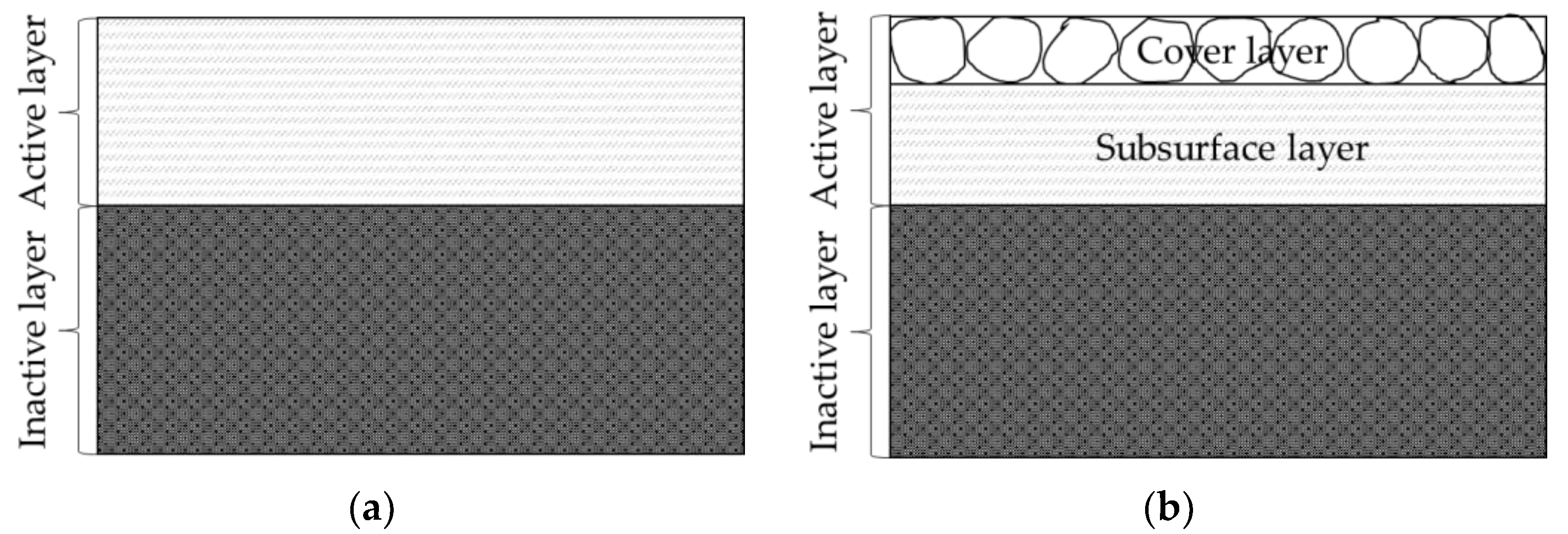
Hirano (1971) suggested the active layer approach [28]. As shown in Figure 1a, this approach classifies the river bed into two layers, an active layer, capable of sediment transport in the time step, and an inactive layer that does not affect the calculation of the sediment transport [24]. The amount of erosion or deposition is applied to the active layer only. This means that the volume of the active layer is a sediment amount that can be transported within one time step. Therefore, the thickness of the active layer is a sensitive variable for computing the amount of sediment transport.
The active layer sorting method has a sensitive effect on the computation of the active layer thickness. Therefore, various methods for computing the active layer thickness were suggested. The Thomas method defined the equilibrium depth as the active layer thickness. Equilibrium depth is the maximum depth that sediment can be transported by the hydraulic energy. A river bed deeper than the equilibrium depth is an inactive layer. Therefore, the active layer thickness is determined by the difference between water depth and equilibrium depth [22]. Equilibrium depth is determined from the relationship between hydraulic energy, bed roughness, and sediment transport intensity, as shown in Equation (2).
where Deq is the equilibrium depth for particle size i, q is water discharge of width, and di is the particle diameter.
Copeland noted that the Thomas method often tends to overestimate the active layer thickness, especially for the sand bed. Copeland suggested that the active layer thickness is 15% of the flow depth or 2d90, whichever is greater. There are several other approaches whereby the active layer thickness is a function of flow depth. Park and Jain (1987) suggested Equation (3) for the determination of active layer thickness [29].
where La is active layer thickness, h is the flow depth, and is a coefficient between 0.1 and 0.2.
Similarly, Orvis and Randal (1987) defined the active layer thickness as a percentage of the water depth [30]. This percentage means that it is a calibration parameter. They found that 20% of the flow depth was appropriate for their application to the Colorado River [24,30].
The Thomas and Copeland methods divide the active layer into a cover layer and an additional subsurface layer. In other words, these methods divide the bed layer into three layers, as shown in Figure 1b. The cover layer is a concept to apply the armoring effect to the calculation of the sediment transport amount, in which the small size material of the bed is eroded first, and then the coarse particles remain to reduce the amount of sediment erosion from the bed. The Thomas and Copeland methods calculate the armoring ratio of the cover layer with the equivalent particle diameter (deq) [22].
The armoring ratio is calculated using the sum of the equivalent particle diameters for each particle size class. The calculated armoring ratio is applied to the calculation of the scouring volume. The armoring ratio by the Thomas method is linearly interpolated in the cumulative coarse equivalent thickness range from the lower boundary where the cover layer has no effect on the scour of the subsurface layer to the upper boundary that completely prevents scouring. The armoring ratio by the Copeland method uses a polynomial line, as shown in Figure 2 [22].
3. Model Setup
3.1. Study Area
To analyze the applicability of the bed sorting method to a river system, the Geum River was considered as the study area. The basin area is 9912.15 km2 and the total channel length is 397.79 km [31]. From Daecheong Dam to the Geum River Estuary bank, 130.47 km of river reach was selected for this study, as shown in Figure 3. According to the investigation of the Ministry of Land Infrastructures and Transport (MOLIT), the shape factor is 0.286. For land use, 61.42% of forest and 19.73% of paddy fields in the study basin [31] were used. The percentages of gravel, sand, silt, and clays are 7.61, 73.48, 12.91, and 6.00%, respectively. This indicated that most soils are composed of coarse grained particles, which are bigger than sand [31]. Because more than 80% of sediment is sand and gravel, the Geum River can be analyzed by applying conventional sediment transport formulas which were developed for non-cohesive material. Therefore, the methodology used for the Geum River can be applicable for the most sand rivers in Korea.
3.2. Numerical Model Design
Input data required to simulate sediment transport are the flow rate or water stage data, topography, and roughness coefficient. In addition, it consists of water temperature data, sediment inflow from the upstream boundary, and grain size distribution data. The upstream boundary condition was flow rate, discharged from the upstream Daecheong Dam, and the observed tide level at the Geum River Estuary bank was used as the downstream boundary, as shown in Figure 4. The upstream flow and downstream tide data were taken from 8 July to 12 July 2016. The downstream boundary was directly affected by the tide. The channel geometry data and roughness coefficient from MOLIT (2016) were applied [31]. MOLIT periodically surveys cross sections and the roughness coefficient of the channel bed to make the master plan of river restoration. A reliable model should be built by using surveyed field data for a plan to manage the river. In order to make a numerical model, 106 cross sections were used along 130.47 km of the study reach. The cross section was measured every 1 km along the river in general. In case of important sections, such as hydraulic structures and confluence, the distance between cross sections were shorter than 1 km. Spacing exceeded 1 km in cases of inaccessible areas. The average distance between the cross section is 1.231 km, and the longest and shortest are 3 km and 0.315 km, respectively. The dynamic equilibrium sediment transport was assumed at the uppermost cross section for the upstream sediment inflow, and the average value of the observed water temperature was used. The bed material size distribution data surveyed by MOLIT (2016) was applied. Bed gradation was not measured for all cross sections. The interpolation method of the bed gradation for cross sections without measured data can be found in the user manual of HEC-RAS. If any cross section is located between one cross section with observed data and the boundary, HEC-RAS copies the bed gradation from the closest cross section with observed gradation [32].
3.3. Model Validation
Simulations were performed using upstream flow and downstream tide levels as boundary conditions, and the applicability of the model was analyzed by comparing the computed and the observed values at three gauging station in the study area, as shown in Figure 5.
In Figure 5, the model underestimated at the first and third stations, while it overestimated at the second station. Along the study reach, three gated weirs were built. The HEC-RAS model has three options for the gate operation based on upstream water surface, the specified reference, and the difference between the upstream and downstream water stages. The specified reference option would be the most accurate for the simulation dealing with the actual gate operation. However, it is difficult to secure the exact time of the opening of the gate, the opening speed, and the time it closed on the particular day in July 2016. In this study, we used the option of differences between water stages. Therefore, it is considered that errors of the simulation results are due to the gate operation in the field.
Indicators used for accuracy analysis were RMSE (Root Mean Square Error) and AGD (Average Geometric Deviation). The indicators were computed by using Equations (4) and (5). The results are summarized in Table 1, indicating that an appropriate model was established.
where and are the observed and computed value, respectively. is the special discrepancy ratio, and is the total number of data.
4. Evaluation of Bed Sorting Methods
4.1. Result of Bed Change with Respect to Bed Sorting Mehtod and Sediment Transport Equation
The results of bed change with respect to sediment transport equation and bed sorting methods were compared. The simulation duration was 500 h with a time step of 60 s.
Two sediment transport equations and three bed sorting methods were applied for sediment transport simulation. According to the literature, the Engelund-Hansen equation is the most suitable for sand transport computation. Because it is a dimensionless equation, it has advantages of application [33,34]. According to the investigation of MOLIT, sediment particles of the Geum river bed are composed of 73.48% sand, and it is one of the representative sand rivers among Korea’s major rivers. Therefore, the Engelund-Hansen equation was selected. The Laursen equation, which is suitable for size ranges between the 0.011 and 29 mm range, was selected as well [22]. This study focused on selecting the proper computational method for the bed armoring process of sand rivers. Regardless of the sediment transport equation, the suitable and stable computation of bed armoring is essential. If the bed armoring is not simulated properly during the erosion process, no sediment transport equation can simulate the sediment movement properly after the erosion process. A total of six cases of simulations with respect to the combination of sediment transport equation and the bed sorting method are indicated in Table 2.
4.2. Capabilty of Simulating Armoring and Grain Size Variation
This study tried to indicate the computed temporal change of median bed material size, d50. Furthermore, d50, d10 and/or d90 are commonly used as representative particle sizes of sediment mixture. The trends for d10, d50, and d90 were similar for this study. Therefore, d50 changes were considered in the evaluation. In order to analyze the applicability of the bed sorting method, the relationship between bed material size change ratio, d50_R, and cumulative river bed volume change during the simulation, dV, was used. The bed material size change ratio is defined in Equation (6).
where d50,f is d50 after 500 h, and d50,i is d50 of initail condition.
The relationships between bed elevation and bed material size changes are visualized in Figure 7, indicating the d50_R and dV for each cross section with respect to combination of simulation options. The left side of 0 on the x-axis indicates the scour, “-” value of dV, the right side indicates deposition, “+” value of dV. The upper side of 1 on the y-axis indicates the increase of d50 and the lower side indicates the decrease of d50. In other words, d50_R > 1 means that the bed material becomes coarser while d50_R < 1 indicates that it is becoming finer.
In general, fine materials are eroded earlier and coarse materials remain in case of erosion, the so-called armoring process. Thus, it is reasonable that bed particles should become coarser during the bed erosion. In Figure 7, the third quadrant indicates scouring with a decrease of d50, with the bed material getting finer, which is not realistic. Therefore, the values on the third quadrant are a clear indicator of the poor capability of simulating the armoring process. The number of cross sections found from the third quadrant is summarized in Table 4. There are several cross sections found from the 3rd quadrant for cases EH_A, L_A, and EH_C, as shown in Figure 7a–c, and Table 4. However, the amounts of scour at cross sections on the third quadrant are very small for these three cases of simulations. One of the examples of the cross section, which has very small scour with bed material becoming finer, is at 41.99 km, as shown in Figure 6e. In this figure, the scour is not significant for cases of EH_A, L_A, and EH_C. In Figure 7a and Table 4, seven cross sections are found in the third quadrant. Cross sections in the third quadrant have a steep slope or reverse slope in terms of thalweg. They are at 55.94, 54.73, 48.5, 43.29, 41.99, 26.14, and 19.18 km. Cross sections at 41.99 and 19.18 km have a steep slope and horizontal slope, respectively. The other five cross sections have a reverse slope. The cross sections at 43.29, 41.99, and 19.18 km have an island. The cross section at 26.14 km has a braided pattern.
In Figure 7d–f, 26.4%, 27.4%, and 22.6% of points were located on the third quadrant respectively, more points than are located on the other cases. This means that the relationship between the erosion phenomenon and the bed grain size change was not explained properly. From Figure 7c,d, the Copeland method has a different result with respect to the sediment transport equation. The Copeland method with the Engelund-Hansen equation simulates bed armoring reasonably, while the Thomas method does not. As shown in Figure 7e,f, the Thomas method is not applicable regardless of the sediment transport equation. On the other hand, the third quadrant is almost empty in Figure 7a,b. This means that the active layer method, the two layer method, reflects the tendency of bed armoring reasonably, regardless of the sediment transport equation.
4.3. Temporal Bed Material Size Variation
Figure 8 indicates the bed material size, d50, on the river bed with respect to the time for all four quadrants, except for Figure 8b, which does not have the third quadrant value. The bed material size of active layer method is stable for all quadrants, as shown in Figure 8a,b, while the Thomas and Copeland methods have oscillatory changes, as shown in Figure 8c–f. This oscillation is a clear sign of instability. Thus, it is only suitable for a specific state river bed sediment transport simulation. Therefore, sufficient investigations should be made to apply the Thomas and Copeland methods to natural state river sediment transport simulations. However, the active layer method is generally applicable with a limited field data set.
When scour occurs, the average particle size typically increases. Because finer particles move earlier than the coarser ones, the finer material flows downstream earlier. Therefore, some cross sections are affected by the fine material, which was eroded from the upstream part. In Figure 8a,b, it is shown that d50 decreases temporarily. However, the simulated bed material size was increased compared to the initial size.
The cross-section in Figure 8 (125.66 km from the downstream boundary) was on the second quadrant for all simulation cases. The cross section at 125.66 km was selected as a representative one of the bed material becoming coarser with scour, which suggests an armoring process. The deposition is dominant for the cross sections in the first of fourth quadrants. The bed materials on the depositional cross sections are directly affected by the characteristics of incoming sediment from upstream. Thus, the temporal change of the bed material size for the cross sections in the first of fourth quadrants varies with location.
5. Summary and Conclusions
Sediment transport computation is a necessary process to solve the river sediment problem. However, there is a lack of research on the applicability of the bed sorting method for river bed armoring algorithms. In this study, simulation stability with respect to the bed sorting method was analyzed by using HEC-RAS. To simulate the sediment transport, a model was constructed using the Geum River, which is a representative sand river, with geometry and river bed characteristics. The model was validated by comparing the observed water level and simulation results. A sediment transport simulation was conducted using this model setup. The performance of the sediment transport model with respect to the bed sorting method was analyzed for six simulation cases. The bed material size changes during deposition or scour processes were compared with respect to the bed sorting method and sediment transport equation. The applicability of the methods was evaluated by considering the ability to simulate the bed armoring process and the temporal bed material size changes. Based on the modeling results, this study concluded the following:
- The bed material size should be increased for eroded cross sections. A comparison of the simulation capability of the armoring process with respect to the bed sorting method indicated that the active layer method, which utilizes two bed layers, simulates the general phenomenon. On the other hand, methods with three bed layers are too sophisticated to simulate armoring processes with general field data.
- Temporal changes of the bed material size variation with the two layer method are reasonable. However, the three layer methods provide oscillatory profiles of bed material size, especially for erosion. Because the three layer methods keep updates of the properties of cover layer for every time step, the oscillatory profile of the bed material size on top of the river bed is inevitable.
- Copeland suggested the applicable particle size range for three layer methods, which means that the bed material size distribution data should be sufficient to apply the three layer method. However, the river bed particle size distribution varies along the reach. In addition, the measurement of bed material size distribution requires effort. Therefore, the three layer method is difficult to be applied to a river with multiple sediment sizes.
- The three layer methods are not very applicable without sufficient field data. In general, a sufficient amount of data is required to solve localized problems. In this case, the field data for the localized simulation may be enough for the application of three layer methods. On the other hand, the management of the entire river system does not require as much of a data set as dealing with a localized problem. Consequently, the two layer bed sorting method is reliable for long reach simulation for engineering purposes. This study focused on a sand river. Further studies with some other river basins may improve the accuracy of the bed sorting prediction.
Author Contributions
Conceptualization, J.L.; methodology, J.A.; software, J.L.; validation, J.L. and J.A.; formal analysis, J.L. and J.A.; investigation, J.A.; resources, J.A.; data curation, J.A.; writing—original draft preparation, J.L.; writing—review and editing, J.A.; visualization, J.L. and J.A.; supervision, J.A.; project administration, J.A.; funding acquisition, J.A. All authors have read and agreed to the published version of the manuscript.
Funding
This work was supported by the National Research Foundation of Korea (NRF) grant funded by the Korea government (MSIT) (No. NRF-2022R1F1A1073059).
Institutional Review Board Statement
Not applicable.
Informed Consent Statement
Not applicable.
Data Availability Statement
Not applicable.
Conflicts of Interest
The authors declare that they have no conflict of interest.
References
- Ahn, J.; Yang, C.T.; Boyd, P.M.; Pridal, D.B.; Remus, J.I. Numerical modeling of sediment flushing from Lewis and Clark Lake. Int. J. Sediment Res. 2013, 28, 182–193. [Google Scholar] [CrossRef] [Green Version]
- Deng, L.; Cai, C.S. Bridge Scour: Prediction, Modeling, Monitoring, and Countermeasures. Pract. Period. Struct. Des. Constr. 2010, 15, 125–134. [Google Scholar] [CrossRef] [Green Version]
- Alemi, M.; Maia, R. Numerical Simulation of the Flow and Local Scour Process around Single and Complex Bridge Piers. Int. J. Civ. Eng. 2018, 16, 475–487. [Google Scholar] [CrossRef]
- Argyroudis, S.A.; Mitoulis, S.A. Vulnerability of Bridges to Individual and Multiple Hazards- Floods and Earthquakes. Reliab. Eng. Syst. Saf. 2021, 210, 107564. [Google Scholar] [CrossRef]
- Khandel, O.; Soliman, M. Integrated Framework for Quantifying the Effect of Climate Change on the Risk of Bridge Failure Due to Floods and Flood-Induced Scour. J. Bridge Eng. 2019, 24, 04019090. [Google Scholar] [CrossRef]
- Briaud, J.; Ting, F.C.K.; Chen, H.C.; Gudavalli, R.; Perugu, S.; Wei, G. SRICOS: Prediction of scour rate in cohesive soils at bridge piers. J. Geotech. Geoenvironmental Eng. 1999, 125, 237–246. [Google Scholar] [CrossRef]
- Mitoulis, S.A.; Argyroudis, S.A.; Loli, M.; Imam, B. Restoration Models for Quantifying Flood Resilience of Bridges. Eng. Struct. 2021, 238, 112180. [Google Scholar] [CrossRef]
- Diaz, E.E.M.; Moreno, F.N.; Mohammadi, J. Investigation of Common Causes of Bridge Collapse in Colombia. Pract. Period. Struct. Des. Constr. 2009, 14, 194–200. [Google Scholar] [CrossRef]
- Wu, T.R.; Wang, H.; Ko, Y.Y.; Chiou, J.S.; Hsieh, S.C.; Chen, C.H.; Lin, C.; Wang, C.Y.; Chuang, M.H. Forensic Diagnosis on Flood-Induced Bridge Failure. II: Framework of Quantitative Assessment. J. Perform. Constr. Facil. 2014, 28, 85–95. [Google Scholar] [CrossRef]
- Grag, R.K.; Chandra, S.; Kumar, A. Analysis of Bridge Failures in India from 1977 to 2017. Struct. Infrastruct. Eng. 2022, 18, 295–312. [Google Scholar] [CrossRef]
- Schaap, H.S.; Caner, A. Bridge Collapses in Turkey: Causes and Remedies. Struct. Infrastruct. Eng. 2022, 18, 694–709. [Google Scholar] [CrossRef]
- Ahn, J.; Yang, C.T. Determination of recovery factor for simulation of non-equilibrium sedimentation in reservoir. Int. J. Sediment Res. 2015, 30, 68–73. [Google Scholar] [CrossRef]
- Karimaee, T.M.; Zarrati, A.R. Sediment transport during flood event: A review. Int. J. Environ. Sci. Technol. 2014, 12, 775–788. [Google Scholar] [CrossRef] [Green Version]
- Woo, H.S.; Kim, W.; Ji, U. Open channel hydraulics, 2nd ed.; Chungmungak: Pajusi, Republic of Korea, 2015; pp. 250–274. [Google Scholar]
- Kwon, B.A.; Hong, K.A.; Woo, H.S.; Rhee, N.A. Bed Elevation Change in a Stream after Weir Removal—A Case Study on Gokreung No.2 Weir in the Gokreung Stream in Korea. In Proceedings of the Korea Water Resources Association Conference, Busan, Republic of Korea, 19–20 May 2008; pp. 1684–1688. [Google Scholar]
- Ahn, J. Introduction of riverbed variation numerical model. J. Water Future 2012, 45, 104–105. [Google Scholar]
- Guo, Q.; Zheng, Z.; Huang, L.; Deng, A. Regularity of sediment transport and sedimentation during floods in the lower Yellow River, China. Int. J. Sediment Res. 2020, 35, 97–104. [Google Scholar] [CrossRef]
- Wang, Z.Y.; Wu, B.; Wang, G. Fluvial processes and morphological response in the Yellow and Weihe Rivers to closure and operation of Sanmenxia Dam. Geomorphology 2007, 91, 65–79. [Google Scholar] [CrossRef]
- Kiat, C.C.; Ghani, A.A.; Abdullah, R.; Zakaria, N.A. Sediment transport modeling for Kulim River—A case study. J. Hydro-Environ. Res. 2008, 2, 47–59. [Google Scholar] [CrossRef]
- Ardiclioglu, M.; Hadi, A.M.W.M.; Periku, E.; Kuriqi, A. Experimental and Numerical Investigation of Bridge Configuration Effect on Hydraulic Regime. Int. J. Civ. Eng. 2022, 20, 981–991. [Google Scholar] [CrossRef]
- Cappato, A.; Baker, E.A.; Reali, A.; Todeschini, S.; Manenti, S. The Role of Modeling Scheme and Model Input Factors Uncertainty in the Analysis and Mitigation of Backwater Induced Urban Flood-Risk. J. Hydrol. 2022, 614, 128545. [Google Scholar] [CrossRef]
- USACE. HEC-RAS River Analysis System Hydraulic Reference Manual, Version 5.0; US Army Corps of Engineers Hydrologic Engineering Center: Davis, CA, USA, 2016. [Google Scholar]
- Brunner, G.W.; Gibson, S. Sediment Transport Modeling in HEC RAS. In Proceedings of the Impacts of Global Climate Change, Anchorage, AK, USA, 15–19 May 2005; American Society of Civil Engineers (ASCE): Reston, VA, USA, 2005; pp. 1–12. [Google Scholar]
- Gibson, S.; Piper, S. Sensitivity and Applicability of Bed Mixing Algorithms. In Proceedings of the World Environmental and Water Resources Congress, Tampa, FL, USA, 15–19 May 2007; Volume 530, pp. 1–12. [Google Scholar]
- Gibson, S.; Sánchez, A.; Piper, S.; Brunner, G. New One-Dimensional Sediment Features in HEC-RAS 5.0 and 5.1. In Proceedings of the World Environmental and Water Resources Congress, Sacramento, CA, USA, 21–25 May 2017; pp. 192–206. [Google Scholar]
- Parker, G. Selective sorting and abrasion of river gravel. I: Theory. J. Hydraul. Eng. 1991, 117, 131–147. [Google Scholar] [CrossRef]
- USACE. HEC-6: Scour and Deposition in Rivers and Reservoirs: Users Manual.; US Army Corps of Engineers Hydrologic Engineering Center: Davis, CA, USA, 1993. [Google Scholar]
- Hirano, M. River-bed degradation with armoring. In Proceedings of the Japan Society of Civil Engineers, Tokyo, Japan, 20 June 1971; pp. 55–65. [Google Scholar]
- Park, I.; Jain, S.C. Numerical Simulation of Degradation of Alluvial Channel Beds. J. Hydraul. Eng. 1987, 113, 845–859. [Google Scholar] [CrossRef]
- Orvis, C.J.; Randle, T.J. Sediment transport and river simulation model. In Proceedings of the Fourth Federal Interagency Sedimentation Conference, Las Vegas, NV, USA, 24–27 March 1986; Volume 2, pp. 24–27. [Google Scholar]
- Ministry of Land Infrastructures and Transport (MOLIT). Master Plan of the Geum River Restoration; Ministry of Land Infrastructures and Transport: Daejeon, Republic of Korea, 2016.
- USACE. HEC-RAS River Analysis Systems User’s Manual Ver. 5.0.; US Army Corps of Engineers Hydrologic Engineering Center: Davis, CA, USA, 2016. [Google Scholar]
- Kim, S.K.; Kim, J.S.; Kim, K.H.; Choi, S.U. Prediction and Historical Analysis of Long-Term Bed Elevation Change in the Mankyung-Gang River. Ecol. Resilient Infrastruct. 2018, 5, 25–34. [Google Scholar]
- Yu, K.K.; Woo, H.S. Comparative Evaluation of Some Selected Sediment Transport Formulas. KSCE J. Civ. Eng. 1990, 10, 67–75. [Google Scholar]
Figure 1.
Schematic of the bed sorting method with HEC-RAS. (a) Two layer method, active layer method; (b) Three layer method, Thomas and Copeland methods (modified from [22]).
Figure 1.
Schematic of the bed sorting method with HEC-RAS. (a) Two layer method, active layer method; (b) Three layer method, Thomas and Copeland methods (modified from [22]).

Figure 2.
Armoring ratio determination process by bed sorting method (modified from [22]).
Figure 2.
Armoring ratio determination process by bed sorting method (modified from [22]).

Figure 3.
Description of study area.

Figure 4.
Water discharge and stage at the up and downstream boundaries, respectively.

Figure 5.
Water surface level comparison between observed data and simulated result (a) First station (126.8 km from the downstream boundary); (b) Second station (101.87 km from the downstream boundary); (c) Third station (98.95 km from the downstream boundary).
Figure 5.
Water surface level comparison between observed data and simulated result (a) First station (126.8 km from the downstream boundary); (b) Second station (101.87 km from the downstream boundary); (c) Third station (98.95 km from the downstream boundary).

Figure 6.
Cross sectional changes: (a) 125.66 km from the downstream boundary; (b) 122.99 km; (c) 81.12 km; (d) 62.32 km; (e) 41.99 km; (f) 36.56 km.
Figure 6.
Cross sectional changes: (a) 125.66 km from the downstream boundary; (b) 122.99 km; (c) 81.12 km; (d) 62.32 km; (e) 41.99 km; (f) 36.56 km.

Figure 7.
Scatter plot between d50_R and dV (a) EH_A; (b) L_A; (c) EH_C; (d) L_C; (e) EH_T; (f) L_T.
Figure 7.
Scatter plot between d50_R and dV (a) EH_A; (b) L_A; (c) EH_C; (d) L_C; (e) EH_T; (f) L_T.


Figure 8.
Temporal sediment size variation at 125.66 km from the downstream boundary (a) EH_A; (b) L_A; (c) EH_C; (d) L_C; (e) EH_T; (f) L_T.
Figure 8.
Temporal sediment size variation at 125.66 km from the downstream boundary (a) EH_A; (b) L_A; (c) EH_C; (d) L_C; (e) EH_T; (f) L_T.


Table 1.
Evaluation of the accuracy of the model.
| 1st Station | 2nd Station | 3rd Station | |
|---|---|---|---|
| RMSE (m) | 0.06 | 0.07 | 0.13 |
| AGD (-) | 1.00259 | 1.00579 | 1.01474 |
Table 2.
Simulation case definition.
| Case | Sediment Transport Equation | Bed Sorting Method |
|---|---|---|
| EH_A | Engelund-Hansen | Active layer method (Two layers) |
| L_A | Laursen | |
| EH_C | Engelund-Hansen | Copeland method (Three layers) |
| L_C | Laursen | |
| EH_T | Engelund-Hansen | Thomas method (Three layers) |
| L_T | Laursen |
Table 3.
Number of deposited or eroded cross sections (total 106 cross sections).
| Case | Number of Deposition Cross-Sections | Number of Erosion Cross-Sections |
|---|---|---|
| EH_A | 60 | 46 |
| L_A | 46 | 60 |
| EH_C | 63 | 43 |
| L_C | 6 | 100 |
| EH_T | 45 | 61 |
| L_T | 37 | 69 |
Table 4.
Number and ratio of cross sections in the third quadrant (total number of cross section is 106).
Table 4.
Number and ratio of cross sections in the third quadrant (total number of cross section is 106).
| Case | Number of Cross Sections in 3rd Quadrant “Scour, Become Finer” | 3rd Quadrant Percentage | Average of dV in 3rd Quadrant | Standard Deviation of dV in 3rd Quadrant | Average of d50_R in 3rd Quadrant | Standard Deviation of d50_R in 3rd Quadrant |
|---|---|---|---|---|---|---|
| EH_A | 7 | 6.6% | −30,820.8 | 22,353.3 | 0.60 | 0.27 |
| L_A | 0 | 0% | - | - | - | - |
| EH_C | 6 | 5.6% | −21,711.5 | 21,251.0 | 0.23 | 0.16 |
| L_C | 28 | 26.4% | −810,803.6 | 504,738.3 | 0.44 | 0.22 |
| EH_T | 29 | 27.4% | −184,628.4 | 126,136.3 | 0.16 | 0.25 |
| L_T | 24 | 22.6% | −673,414.6 | 311,869.8 | 0.63 | 0.24 |
Disclaimer/Publisher’s Note: The statements, opinions and data contained in all publications are solely those of the individual author(s) and contributor(s) and not of MDPI and/or the editor(s). MDPI and/or the editor(s) disclaim responsibility for any injury to people or property resulting from any ideas, methods, instructions or products referred to in the content. |
© 2023 by the authors. Licensee MDPI, Basel, Switzerland. This article is an open access article distributed under the terms and conditions of the Creative Commons Attribution (CC BY) license (https://creativecommons.org/licenses/by/4.0/).
Share and Cite
MDPI and ACS Style
Lee, J.; Ahn, J. Analysis of Bed Sorting Methods for One Dimensional Sediment Transport Model. Sustainability 2023, 15, 2269. https://0-doi-org.brum.beds.ac.uk/10.3390/su15032269
AMA Style
Lee J, Ahn J. Analysis of Bed Sorting Methods for One Dimensional Sediment Transport Model. Sustainability. 2023; 15(3):2269. https://0-doi-org.brum.beds.ac.uk/10.3390/su15032269
Chicago/Turabian StyleLee, Jeongmin, and Jungkyu Ahn. 2023. "Analysis of Bed Sorting Methods for One Dimensional Sediment Transport Model" Sustainability 15, no. 3: 2269. https://0-doi-org.brum.beds.ac.uk/10.3390/su15032269
Note that from the first issue of 2016, this journal uses article numbers instead of page numbers. See further details here.