Streamlining Building Energy Modelling Using Open Access Databases—A Methodology towards Decarbonisation of Residential Buildings in Sweden

Abstract

The building sector is a major contributor to greenhouse gases, consuming significant energy and available resources. Energy renovation of buildings is an effective strategy for decarbonisation, as it lowers operational energy and avoids the embodied impact of new constructions. To be successful, the energy renovation process requires meaningful building models. However, the time and costs associated with obtaining accurate data on existing buildings make large-scale evaluations unrealistic. This study proposes a methodology to streamline building energy models from open-access datasets for urban scalability. The methodology was tested on six case study buildings representing different typologies of the Swedish post-war construction period. The most promising results were obtained by coupling OpenStreetMap-sourced footprints with energy performance declarations and segmented archetypes for building characterisation. These significantly reduced simulation time while retaining similar accuracy. The suggested methodology streamlines building energy modelling with a promising degree of automation and without the need for input from the user. The study concludes that municipalities and building owners could use a such methodology to develop roadmaps for cities to achieve carbon neutrality and evaluate energy renovation solutions. Future work includes achieving higher accuracy of the generated energy models through calibration, performing renovation analysis, and upscaling from individual buildings to neighbourhoods.

1. Introduction

Globally, the building sector accounts for 40% of energy use, corresponding to 36% of global greenhouse gas emissions in Europe [1]. Roughly three-quarters of buildings in the EU are energy inefficient, yet 85–95% of today’s buildings will still be in use in 2050 [2] when the EU aims to achieve climate neutrality [3]. More than one-third of the EU’s buildings are over 50 years old, but the renovation rate is lower than 1% per year [3,4]. Sweden aims to reach climate neutrality by 2045 [5]. Moreover, 23 Swedish pioneer municipalities—together accounting for 40% of Sweden’s population—are even more ambitious and aim for that goal by 2030 [6]. As in many European cities, many municipalities in Sweden experienced the rapid growth of residential neighbourhoods during the post-war period. Those extensive neighbourhoods now need renovation. Thus, large-scale energy renovation opens a window of opportunity to reduce building operational energy and, therefore, help to decarbonise Swedish cities.

Making an informed decision on building renovation is challenging [4]. Stakeholder interests, combined with uncertainty regarding the final performance, often impede deep energy renovations [4,7,8,9]. Building energy modelling is advantageous in assessing the impact of different renovation scenarios through numerical simulations, thereby providing evidence to the debate among decision makers [4,10,11]. For energy renovations, energy models of large building stocks are particularly beneficial for both increasing the actual renovation rate of buildings and evaluating building impacts on a larger scale [12].

Numerous methodologies and tools have been developed to scale energy modelling from single buildings to urban models [13]. Urban energy building models (UBEM) provide users with the energy demand of the building stock, including baseline calibration [14], energy efficiency scenario evaluation, and other important analyses such as the economic and environmental impact during the future life cycle of the buildings [15,16,17,18].

Urban building energy modelling has been thoroughly reviewed [19,20,21] and is usually divided into two modelling approaches: top–down and bottom–up. Top–down urban models describe buildings at a general level, using large datasets that are not building-specific. These datasets contain factors that drive the energy performance of buildings [22,23], such as technical [9,24], socio-economic [25,26,27], or physical factors [28]. However, these datasets are based on reported data from the past, making top–down UBEMs useful for large-scale assessments but not ideal for predicting future scenarios. Further, top–down building modelling lacks the necessary granularity to enhance detailed numerical simulations. Bottom–up building modelling, on the other hand, uses building-specific models that can support detailed numerical simulations to predict the future energy performance of buildings. The energy modelling can be accomplished through statistical methods or by actual thermal modelling of the buildings. Both methods are driven by databases on building constructions such as envelope materials, window structure, HVAC systems and user behaviour. However, suitable databases are often non-existent or difficult to access, and energy modelling knowledge is needed to process them.

Organising the input for simulation is the key focus of this paper, which aims to simplify this task as it is considered the major obstacle to obtaining bottom–up urban models. The urban modelling process is time-consuming and complex, even for an expert user. To obtain a reliable energy model, methods have been sought to break down the process into three main subtasks: (1) organise the input for the simulation, (2) generate and run the thermal model, and (3) validate the results (calibration) [29]. Within the scope of the energy modelling process, this paper does not pay much attention to the second and third subtasks, which are already well established and supported by numerous studies and literature. Rather, it focuses on the first step, which is considered the major obstacle to large-scale assessments.

In recent years, many bottom–up generated urban models have gained momentum [30]. Generally, bottom–up UBEM is built by merging large datasets that describe buildings and user patterns. It is common to use available geographical information systems (GIS) datasets to generate building geometries, often referred to as 3D city models [31,32,33]. In Sweden, however, the standard for generating and managing 3D city models is still under development [31,34], which is a major barrier to automating UBEM generation. Moreover, due to the lack of a standard, access to 3D city models is not centralized and each city decides on the level of detail or the tools they use to generate these models. [31,33,34].

Unlike 3D urban models, building footprints are freely accessible worldwide through Google Maps, OpenStreetMap or other web mapping platforms. The OpenStreetMap project is a global open GIS database that offers a free download service for building footprints in OSM extension. In Sweden, Lantmäteriet, the Swedish mapping cadastral and land registration authority, offers public geodata services that include building footprint datasets, typically as shapefiles (SHP) [35]. Those datasets can be partially obtained on the website. Full access is given for research through the Geodata Extraction Tool (GET) [36] offered by the Swedish University of Agricultural Sciences, SLU.

Building geometry modelling can be obtained from the “slicing” of a 3D solid or from extrusion of the building footprint. Figure 1 summarises the cutting (A) and extrusion (B) methods graphically.

The first modelling method (A) employs existing 3D solid models, such as City GML or City JSON, to create building solids. These 3D models represent the geometry, topology, semantics, and appearance of real-world city objects, such as buildings, in a digital format. Building solids can also be constructed from other types of geospatial data, such as point clouds based on laser scanning (LIDAR) or raster datasets (aerial photographs). Point clouds are dense collections of 3D points that can be used to reconstruct the 3D geometry of buildings. Raster datasets, such as aerial photographs, can be used to extract building footprints and other features. In this case, if thermal zones are required for each level, the solid is sliced to define the different floors.

The second modelling method (B) uses the building footprint, which represents the outline of the building at ground level, to extrude each level and stack them on top of each other. This method can be used when the detailed 3D geometry of a building is not available. The choice between the two methods depends on the level of detail required for the simulation and the available dataset. The City GML [37,38,39] modelling standard organises the level of detail (LOD) of the building geometry, into four consecutive groups (LOD0–3). LOD0 represents the lowest level of detail, with only the building’s footprint available. LOD1 represents a simplified exterior volume with a flat roof [34,40], and it is typically used for thermal modelling of buildings [21,38,41,42]. LOD2 and LOD3 represent increasingly detailed exterior and interior geometries, respectively. The use of LOD1 allows for a balance between computational efficiency and accuracy of the simulation results [40,43].

Energy models from building footprints are often more convenient as they require less post-processing to become a simulation-friendly thermal model compared to the first method. This is because the building footprint already represents the outline of the building at ground level and can be directly used to generate the thermal model. In contrast, the detailed 3D geometry of the building may require additional processing steps, such as simplification or cleaning, before it can be used for simulation.

For building energy modelling, the thermal characterisation of existing construction, active systems and usage patterns is often a complex task. At present, manual inspection or the use of databases is necessary to obtain the thermal model of the building. When moving to urban models, thermal characterization gets more complicated as the amount of data to be filled in becomes too large.

At the European level, there are several databases that can provide valuable modelling input data. These include the EU Building Stock Observatory (BSO) [44], the TABULA and EPISCOPE research projects [45,46], and Energy Performance Certificates (EPC) [47,48,49]. Additionally, EPCs can be used for benchmarking the energy performance results of the UBEMs.

In Sweden, there are several databases that facilitate characterisation of the existing residential building inventory. This includes the BETSI database, which was created following a survey on the technical status of 10,000 buildings by the Swedish National Board of Housing during the heating season in 2007–2008. The building selection process in the BETSI study was careful to be representative of the residential building stock in Sweden. Surveyed buildings were split between single-family houses and multi-family buildings. Within the latter group, a segmentation was made according to the year of construction: before 1960, 1961–1975, 1976–1985, 1986–1995 and 1996–2005. Additionally, each age group period was subdivided into seven building typologies, resulting in 35 archetypes. BETSI provides valuable data on building dimensions, construction details, HVAC systems, type and percentage of openings according to facade orientation, roof and basement typology, as well as the need for renovation and work performed to date, without being an exhaustive list. Additionally, the cross-industry program for standardisation and verification of the energy performance of buildings, SVEBY [50], has conducted multiple studies on Swedish users’ patterns and input values [51] for accurate energy modelling of the Swedish building stock.

However, current approaches for building energy modelling at both the building and neighbourhood level are not yet ready to provide fully automated energy modelling. This is due to limitations in data management and interoperability, and a lack of suitable methods for large-scale assessments that are technologically ready to be implemented. These limitations have been recognized by several studies [52,53,54,55,56].

This research aims to fill this gap by providing a new methodology to generate building energy models for multi-dwelling residential buildings or groups of buildings in Sweden. The target group of the methodology is users without prior knowledge of energy modelling, such as building owners and municipalities. To ensure ease of use, priority was given to technological and interoperability readiness, as well as free access to the tools and datasets employed. To demonstrate the effectiveness of the proposed methodology, six case study buildings were selected from different geographical locations in Sweden, built during the period 1961–1975, and representing different building typologies.

2. Methods

This section describes the proposed energy modelling methodology. Section 2.1 describes the overall modelling workflow of the flexible input process whereby the user can customise the default generated building energy model needed. Section 2.2 describes the generation of the building geometry, which is then thermally and functionally characterised into a suitable energy model, as described in Section 2.3. Finally, the selected case study buildings are presented in Section 2.4.

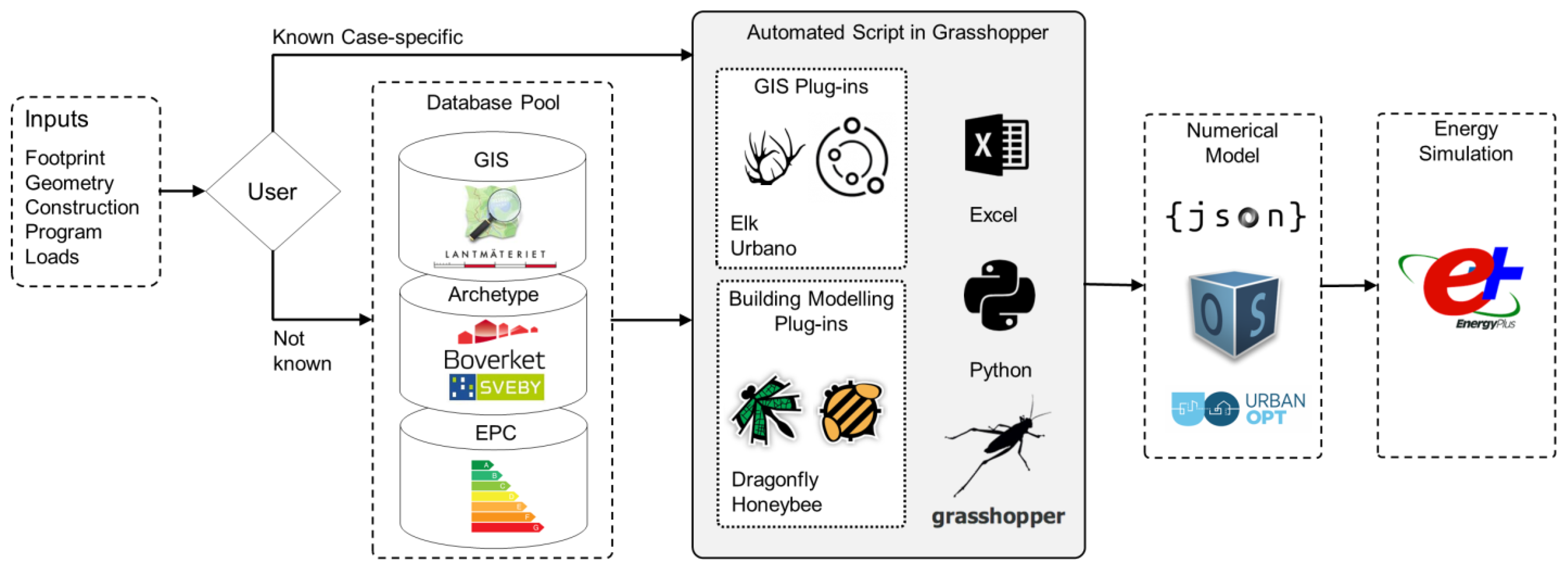
2.1. Overall Modelling Workflow

Figure 2 summarises the entire modelling process, describing the script developed to automate a building energy model using the Grasshopper visual programming environment coupled with the CAD modeller Rhinoceros 3D. The process starts by asking the user to define specific data. When input data are unknown or unavailable for the different input needed, characterisation is made through a predefined age and typology archetype segmentation from a database pool, including geographic information systems (GIS), thermal properties and energy performance certificate (EPC) datasets.

The Grasshopper script automates the process of finding the closest building footprint to a selected address or building. The building footprint is defined as a closed polygon with embedded metadata for each point, such as geographical coordinates, building, block, neighbourhood and others, following predefined attribute categorisation of the map features [57]. Although the amount and quality of the metadata associated with each building footprint in OpenStreetMap may vary, points defining building entrance and address are generally available. The address for each staircase is used to access the building’s corresponding energy performance certificates (EPC).

The data obtained from the EPCs is used to adjust the geometrical model, which is built from either OSM or SHP footprints. If more precise data are not available from the user, the number of stories is obtained from the EPC, and each level’s height is an average value obtained from the BETSI database.

The thermal characterization of the building is then performed using segmented archetypes related to the building’s age and typology. Once the numerical model is ready, it can be stored as a file (json) or sent for direct simulation to EnergyPlus through OpenStudio using different energy modelling plugins for Grasshopper 3D to create the numerical model.

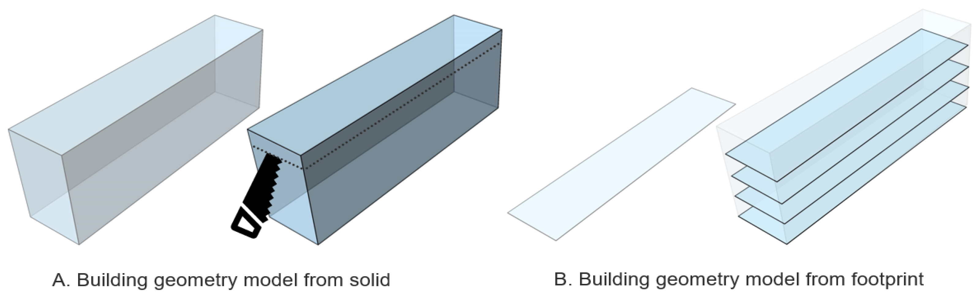
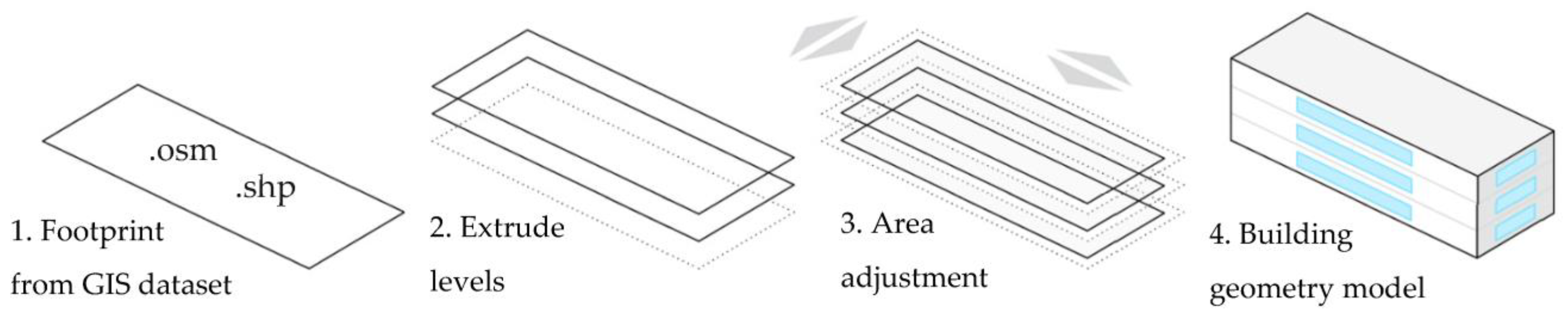
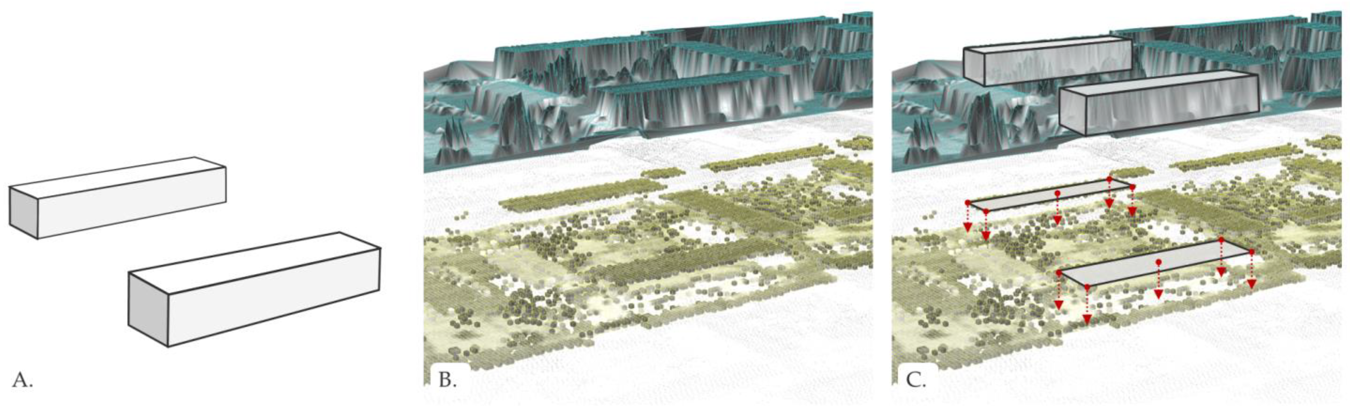
2.2. Building Geometry

For the building geometry construction, average floor-to-floor heights for each level (ground floor, intermediate floor(s) and, last floor) and the window-to-wall ratio (WWR) for each façade were taken from BETSI’s archetype. Once the whole building geometry was generated, the resulting total heated floor area was benchmarked with the heated area defined in the EPCs. The geometry model was adjusted to match the EPC total heated floor area. Employing a single-objective optimisation algorithm, the necessary building footprint offset to be made to the footprint of the building was obtained. This allowed automating the fitting even with a complex building footprint geometry. Figure 3 provides an overview of the process for generating the building geometry.

The datasets explored for generating building footprints included the cadastre building footprints from building permits (SHP files) and OpenStreetMap footprint points with embedded map features (OSM files); both are open access and freely available. Additionally, a surface model was used from Airborne Laser Scanning (LAS/LAZ files), although only for verification of significant deviations of volume and building height, not supporting the building geometry modelling, as further explained in the paragraph below.

Different tools and processes were explored to generate the building geometry from open access geodata. After an exhaustive search in the two main Grasshopper 3D tool libraries [58,59], 49 tools were identified, out of which 39 were open access and thus further investigated. After testing, Elk, Urbano and Volvox Grasshopper plug-ins were incorporated.

Table 1. Selected tools supporting GIS integration within the Grasshopper environment.

Tool Name	Description	Function	Level of Automation
ELK	Grasshopper plug-in	Point and metadata from OSM files	Low, files uploaded manually
URBANO	Grasshopper plug-in	Point and metadata from OSM, SHP and LAS files	Medium, OSM automated downloading
VOLVOX	Grasshopper plug-in	Point cloud manipulation engine from LAS/LAZ files	Low, files uploaded manually

describes the selected GIS tools.

As listed in Table 1, Elk was selected for point and metadata extraction from OSM (OpenStreetMap) files due to its simplicity and good operability. Urbano adds automation features to the OSM download and supports both Shapefile and Lidar formats, which can be imported and positioned on the correct coordinates using a translation vector, referencing data previously sourced from OpenStreetMap. Volvox was employed to validate the volume and height of the geometries obtained manually. As shown in a graphical summary in Figure 4, the different building geometries (A) overlapped with the “real” 3D surface model obtained from the Airborne Laser Scanning, LIDAR (B) dataset to ensure there were no significant discrepancies through manual inspection (C).

Differences in height between the generated geometry and point-cloud dataset across the six neighbourhoods investigated did not exceed 1.3 m, while differences in volume were up to 46% greater in neighbourhood F (Ällingavägen), with L-shaped buildings. The building geometry generation using Elk and Urbano was considered reasonably accurate. Due to its complexity, the Volvox plug-in was not integrated into the modelling automation. It is reserved for verification of specific cases where the discrepancies between EPC surfaces and the model obtained are considerable. Therefore, Volvox and point-cloud generated surfaces are not evaluated in the Results and Discussion sections.

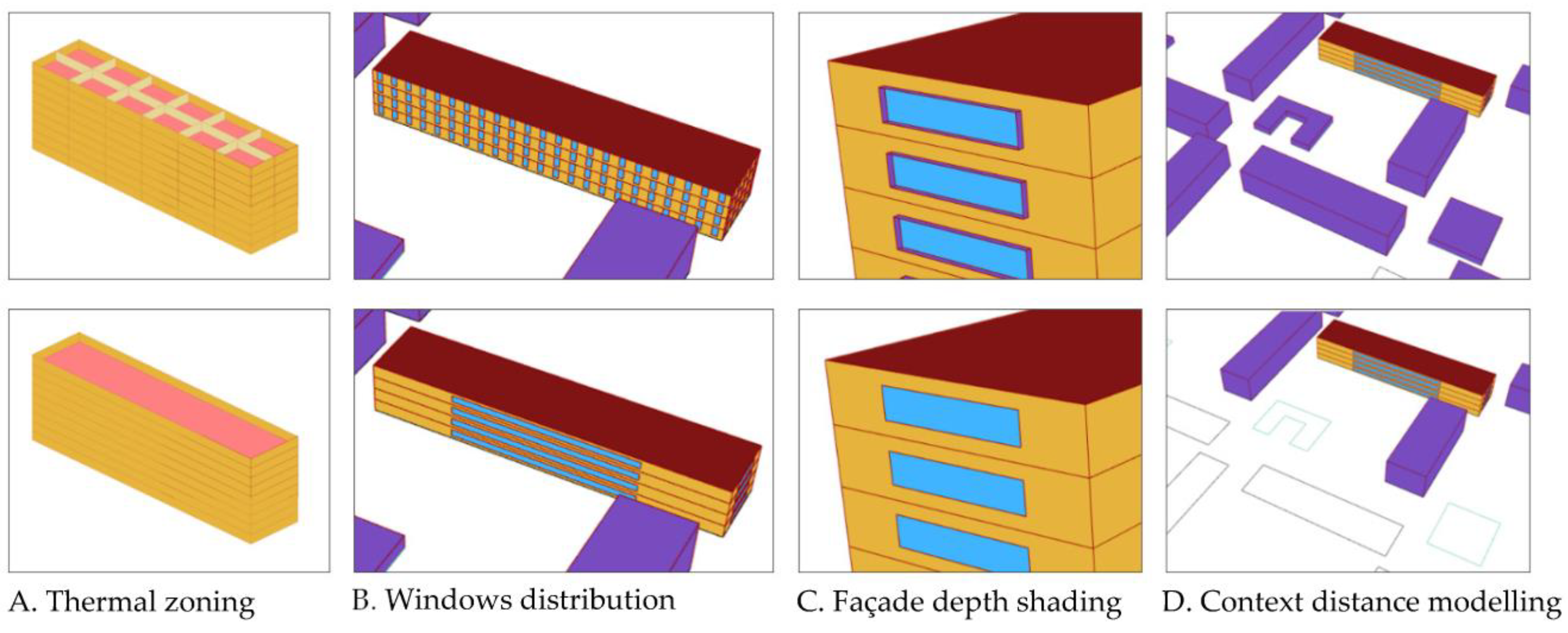
2.3. Building Thermal Model

The next step in the modelling process was to assign the envelope characteristics that influence the energy performance of the building. Following the previously mentioned process, average values from the archetype database were taken according to the year of construction of the building and its building typology.

Table 2. Basic input needed on the building envelope predefined by BETSI [49] archetype datasets when unknown.

Envelope Thermal Properties	Unit	Building Element	Type of Input	Source
Window to wall ratio (WWR)	%	North, east, south, west façades	Average	BETSI
G-Value	Fraction	All windows	Average	BETSI
U-Value glazing materials	W/m²K	Apertures	Average	BETSI
U-Value opaque materials	W/m²K	Roof, façade, ground	Average	BETSI
Thermal mass	No predefined thermal mass is assigned—“No mass material” is selected

summarises the envelope thermal properties assigned to the model. The affected building elements, type of input and source used are detailed.

Once the static properties of the energy model are defined, dynamic characterisation of the model is needed to run an initial dynamic simulation. Building program and loads used to define the operation model of the building are summarised in

Table 3. Default input sourcing that defines the building operation model.

Building Program	Unit	Type of Input	Source
Occupancy density	People/m2	Average	Boverket, Sveby
Occupancy schedule	Hourly	Monitored/Archetype weighted	Sveby
Lighting density	W/m2	Recommended	Boverket, Sveby
Lighting schedule	Hourly	Archetype weighted	Boverket, Sveby
Equipment density	W/m2	Recommended	Boverket, Sveby
Equipment schedule	Hourly	Monitored/weighted	Sveby, ELIB [60]
Infiltration rate	l/s	Monitored/weighted	Sveby, ELIB
Infiltration schedule	Hourly	Constant	Boverket, Sveby, ELIB
Ventilation rate	l/s/m2 HFA	Building code, Monitored/weighted	ELIB
Ventilation schedule	Hourly	Constant	ELIB
Ventilation system	l/s/m2 of façade	F, AF, FT, FTX	BETSI
Heating setpoint	Celsius	Monitored/weighted	Sveby
Heating schedule	Hourly	Constant heating season	Sveby
Cooling setpoint	Celsius	Need 27° Celsius	Sveby
Cooling schedule	hourly	None	Boverket, Sveby, ELIB

.

The data sources used in this case were taken from official recommendations for the simulation input of residential buildings in Sweden (Boverket, Sveby). Data related to the operation of the building were based on several previous measurements [60]. These were considered independent of the age and typology of the building. Since there are no data from infiltration tests in the databases, an average value for the infiltration rate was used. The type of ventilation, natural exhaust, forced exhaust, supply and exhaust, or supply and exhaust with heat recovery, were taken from specific building EPC.

The Grasshopper visual programming platform in the Rhinoceros 3D modeller was used to implement an all-encompassing script which automated the BEM generation within one environment. Moreover, this allowed for an optimisation process with reasonable time allocation per energy simulation iteration, as no need for manual post-processing was needed between different tools. The building model was obtained using Dragonfly (https://0-doi-org.brum.beds.ac.uk/10.3390/en14185931) and Honeybee from the Ladybug Tools Grasshopper plug-in, connecting with the above input and assigning the specific weather data. Several measures were evaluated to simplify the model and, thus, reduce simulation time for each iteration. Keeping reasonable time per iteration was needed to allow scalability of the model in future work, both for evaluating more buildings at the urban level and assessing many renovation scenarios for each building. Some of the simplification measures that were considered are illustrated in Figure 5.

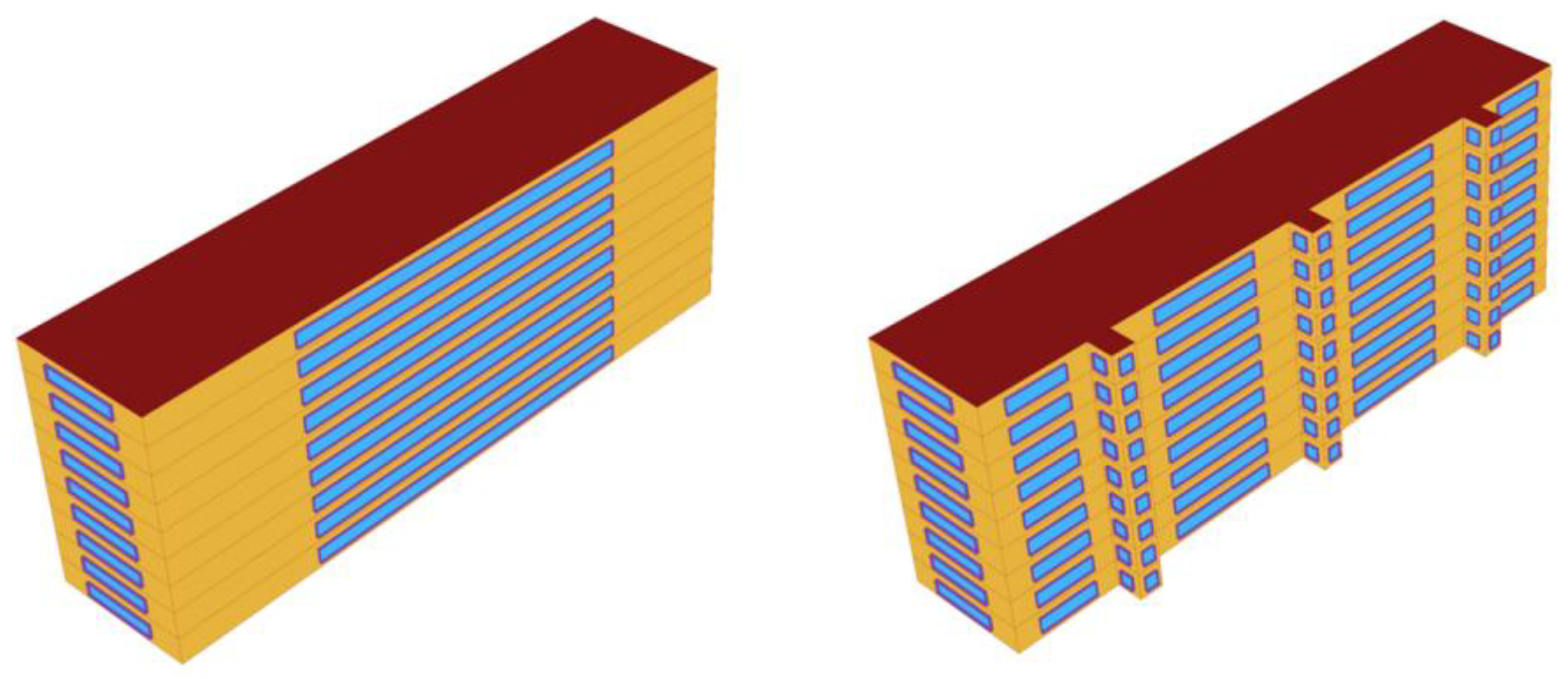
• The study evaluates the effect of using one thermal zone per floor instead of one per individual dwelling unit, as the necessary detailed plans for each floor are not available;
• Windows obtained as a ratio of the exterior façade (window-to-wall ratio) could be modelled as a single window per level and façade or distributed evenly;
• Depth or thickness of the existing façade and its relative position to the window was also evaluated;
• Impact of considering different radius distances for the modelling of the context (e.g., other buildings) around the building.

2.4. Case Studies

The selected neighbourhoods are from the post-war construction period (1961–1975) since they contain a significant share of the building stock in Sweden and need renovation. For this period, three out of the seven different building typologies available were selected, including different numbers of stories. Those typologies were selected based on a statistical representative within the construction period. However, the archetype characterization seen in the previous Building Thermal Model section was averaged for the entire age group, disregarding building typologies. In order to limit uncertainty, the selected buildings are in the same climatic zone (south of Sweden), do not have a basement, and have no upgraded forced exhaust ventilation system. No further data were available for the buildings besides those obtained from the databases mentioned above. A synopsis of the selected case studies can be found in

Table 4. Neighbourhoods selected as case studies.

Neighbourhood	Location	Building Typology	Number of Stories	Construction Year	Total HFA/m2 Building
A. Fagottgränden	Lund	Low-rise slab	2	1970	1257
B. Markurellagatan	Gothenburg	Low-rise slab	3	1970	1476
C. Kadettgatan	Helsingborg	Low-rise slab	4	1968	2948
D. Siriusgatan	Gothenburg	High-rise slab	7	1970	6211
E. Rosengård	Malmö	High-rise slab	9	1969	6800
F. Ällingavägen	Lund	Non defined/Other	5	1966	3026

.

3. Results

The results of implementing the methodology for geometry and thermal modelling of the case studies are described in Section 3.1 and Section 3.2, respectively.

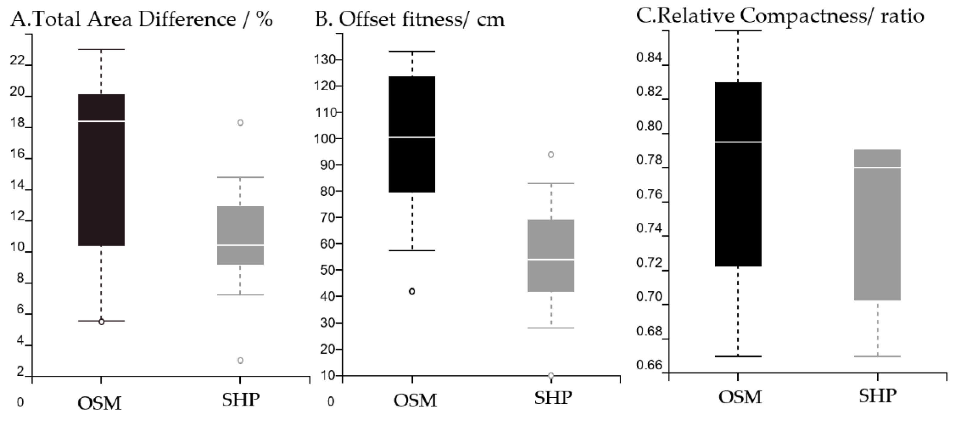
3.1. Geometry Modelling of Case Studies

The generation of building geometry by using building footprints from OpenStreetMap (OSM) and cadastral shapefiles (SHP) was successful in all neighbourhoods.

Table 5. Building geometry benchmark of OpenStreetMap (OSM files) building footprints against (energy performance certificates, EPC) for case studies A to F.

Neighbourhood		Geometry Visualisation from SHP	Source	Total HFA m2	Offset Needed cm	HFA Difference %	Relative Compactness Ratio
A	Fagottgränden		EPC	1257	-	-	-
			OSM	1302	74	3.5	0.68
			SHP	1503	84	16.3	0.66
B	Markurellagatan		EPC	3226	-	-	-
			OSM	3549	32	6.2	0.65
			SHP	3256	0	1	0.65
C	Kadettgatan		EPC	2948	-	-	-
			OSM	3772	123	21	0.77
			SHP	3330	62	11.4	0.77
D	Siriusgatan		EPC	6211	-	-	-
			OSM	7593	116	18.2	0.82
			SHP	6858	51	9.4	0.77
E	Rosengård		EPC	6800	-	-	-
			OSM	8278	107	17.8	0.84
			SHP	6804	37	7.5	0.77
F	Ällingavägen		EPC	3026	-	-	-
			OSM	3549	68	15	0.78
			SHP	3256	30	7	0.75

displays the results obtained. When using OSM footprints, the resulting areas were generally larger, with differences ranging from 3.5% to 21% compared to the area obtained from the energy performance certificates (EPC). The offset needed to adjust building footprints and match EPC’s total heated floor area ranged from 32 to 123 centimetres.

Differences in the resulting heated floor area (HFA) obtained were smaller when using SHP building footprints. No adjustment to the building footprint was necessary for neighbourhood B, as the area was practically the same as that found in the EPC. However, in two cases, neighbourhood A and C, the area difference was 16.3% and 11.4%, respectively.

Figure 6 compares the distribution of area difference between the model and EPC, the offset applied to the building footprint to fit EPC area, and the relative compactness ratio of resulting geometries from OSM and SHP footprints.

The total area difference boxplots show that the use of Shapefiles resulted in geometries with an area difference of less than 16% compared to EPC. Most results were targeted between 7% and 11%. With the OSM dataset, the area difference reached a maximum of 21%, with a wider dispersion of results. The offset required for area adjustment with SHP dataset ranged from no adjustment to a maximum of 80 cm, with a concentration of results in the 30–60 cm range. In contrast, the offset with OSM ranged from 30 cm up to 1.2 m. The different complexities of the buildings affected both datasets similarly, but a more compact range of the results of total area difference and offset required was observed using cadastral shapefiles.

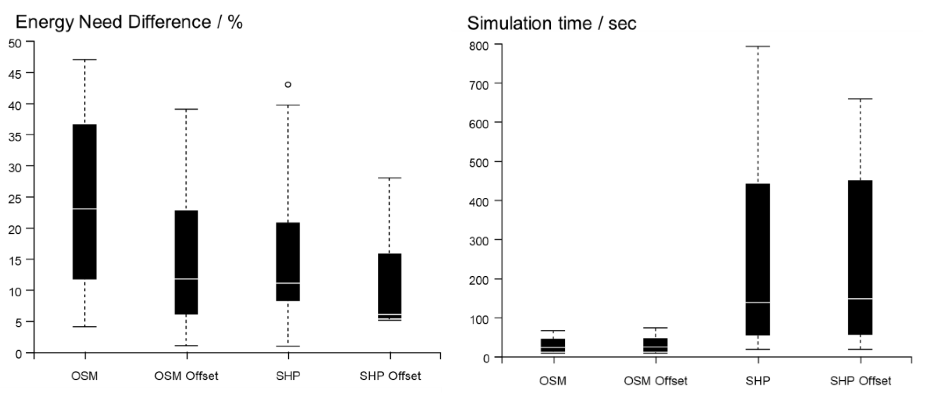
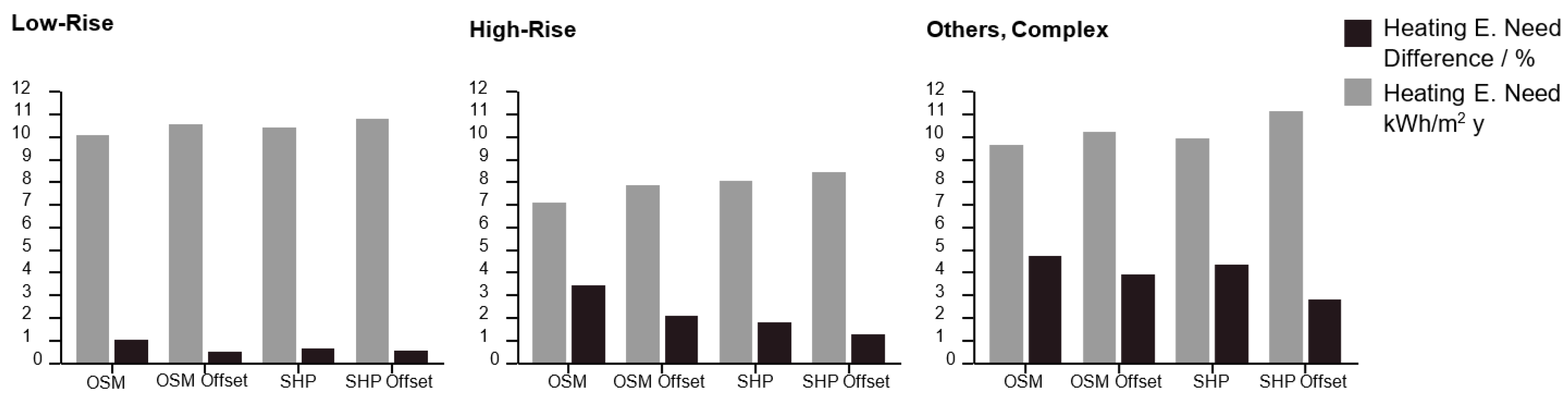
3.2. Thermal Modelling of Case Studies

The thermal characterization using the proposed methodology resulted in satisfactory generation of the numerical building model and subsequent energy simulation in EnergyPlus.

Table 6. Averaged results comparison of the different simplification measures tested using OpenStreetMap and shapefile sourced building footprints. (*) The default context distance of 50 m was retained for the comparison of results when considering other radius distances for modeling the building context.

Measure	Heating Energy Need Average Difference/%		Simulation Time Average Difference/%
	OpenStreetMap	Shapefile	OpenStreetMap	Shapefile
A. Thermal zone per level	0.9	1.2	−625	−728
B. Grouped windows	−0.6	0.1	−35.4	−14.7
C. Adding façade depth	2.8	4.7	122	506.7
D10. Context 10 m	−1.6	NP	1.3	NP
D25. Context 25 m	−0.9	NP	−1.1	NP
D50. Context 50 m	0 *	NP	0 *	NP
D75. Context 75 m	0.1	NP	0.9	NP

summarises the energy performance accuracy and simulation times obtained during the optimisation process of the thermal modelling.

The most significant simulation time savings were achieved when using a single thermal zone per level, with reductions of 625% and 728% using OSM and SHP, respectively, while heating energy increased by around 1%. Grouping windows had a negative impact on the energy performance of 0.6% with OSM and barely any impact on the SHP model. Simulation time was reduced by an average of 35.4% to 14.7%. Modelling the façade’s depth resulted in simulations that were up to 500% slower and increased heating energy by 5%. Finally, the impact of modelling different contexts (adjacent buildings, vegetation, etc.) at different distances around the building was verified, and a maximum radius of 50 m (D₅₀) was defined as a “common practice” value and used as a reference for comparison. The default context radius of 50 m was retained as the standard, but it should be increased where necessary, for instance, if the primary source of obstruction is beyond 50 m. Once the above-described settings for the energy modelling were optimised, the procedure was tested on specific case studies with the following settings: a single thermal zone per storey, grouped windows per storey and façade orientation, no façade depth shading around the apertures, and context within 50 m.

Table 7. Energy performance for heating and simulation time results obtained across the studied neighbourhoods. The offset values are referring to heating energy based on adjusted building footprints to match the EPC’s total heated floor area.

Neighbourhood Building Typology	Source	Heating Energy kWh/m2/y	Heating Energy Difference/%	Simulation Time/Seconds
Fagottgränden	EPC	126	-
	OSM	121	4	14
	OSM offset	127.4	1	14
	SHP	125	0.9	55
Low-rise slab	SHP offset	133	5.2	60
B. Markurellagatan	EPC	81	-
	OSM	123.5	10	9
	OSM offset	126.4	7.5	9
	SHP	126.7	7.2	53
Low-rise slab	SHP offset	128.1	6	52
C. Kadettgatan	EPC	65.5	-	-
	OSM	56.2	16.5	12
	OSM offset	62.1	5.5	11
	SHP	59.1	11	18
Low-rise slab	SHP offset	62.4	5	18
D. Siriusgatan	EPC	99	-	-
	OSM	71	39	32
	OSM offset	79	25	33
	SHP	79.5	24	792
High-rise slab	SHP offset	83	19	657
E. Rosengård	EPC	90	-	-
	OSM	70	29.4	50
	OSM offset	77.5	16	52
	SHP	81	11	516
High-rise slab	SHP offset	85.1	6	522
F. Ällingavägen	EPC	142	-	-
	OSM	96	47	66
	OSM offset	102	39	72
	SHP	99	43	222
Others, Complex	SHP offset	111	28	234

displays the results of the energy performance and simulation time according to the dataset used for importing the building footprints.

The measured heating energy in the EPCs was used to benchmark the percent difference between the energy models obtained from the two datasets before and after the area fitting of the building’s footprint. As shown in Figure 7, results show that the gap in energy performance was lower when using SHP (5% to 25% after area adjustment). Nevertheless, the simulation time increase when using SHP was up to eight times higher compared to OSM.

The simulation time remained below one minute for OSM, except in neighbourhood F, where it was 72 s due to the increased complexity of the buildings. For SHP, the longest time was 657 s per building in the Siriusgatan neighbourhood (D) (see Figure 7). The high-rise slab buildings resulted in the most time-consuming energy simulations when using SHP, while the more geometrically complex neighbourhood performed similarly for OSM and shapefile energy models. The low-rise slab neighbourhoods had the fastest energy simulations and the closest results to the EPCs, with the best performance across all building typologies when using OSM-based energy models. Figure 8 shows that the modelled heating need had the lowest deviation compared to measurements from EPCs for low-rise buildings.

4. Discussion

The results of the study contribute to quantifying the trade-off between energy results accuracy and simulation time when using different approaches to generate building energy models with no input data from users. The OpenStreetMap (OSM) GIS database was found to be suitable for modelling low-rise buildings. The accuracy of the generated heated floor area and heating need was found to be similar between OSM and shapefile (SHP) cadastre GIS database, so OSM was preferred for this building typology due to the faster simulation time. The higher compactness and less complex geometry of low-rise buildings could also explain the lower deviation between the modelled heating area and resulting heating need compared to measurements from energy performance certificates (EPCs) for low-rise buildings. The good performance for low-rise buildings is further supported by the fact that this typology represents 58% of the BETSI dataset for the analysed period. This means that assumptions about the thermal properties of the building envelope and ventilation systems are more likely to be accurate when modelling low-rise buildings. Additionally, low-rise buildings are the most common typology for residential buildings in Sweden, so this result is relevant for scaling up future studies on national-level renovation scenarios where accuracy and low computational cost of thermal modelling are essential.

Contrarily, other building typologies, such as high-rise and complex buildings showed significant differences between the modelling procedures using OSM and SHP. These buildings have more complicated footprint geometries, which explains the larger deviation when modelled using a more simplistic method such as OSM. In Figure 9, a visual comparison is shown of a high-rise building modelled using the OSM footprint on the left and the cadastral shapefile on the right.

The difference between the footprints is due to the fact that high-rise slab buildings often have buffered entrances attached to each staircase, which are not captured in the OSM data but are present in the cadastral shapefile database. When using the SHP data with the extrusion modelling procedure, it is important to target a higher level of detail (LOD), such as LOD 1.3, which provides geometric detail of the outer perimeter per level. Otherwise, the complexity can hinder the effectiveness of simplification measures such as grouping the windows per façade. This issue was seen during the optimization process of the geometry model (Figure 5), as the implementation of grouping apertures proved to be twice as effective in reducing simulation times with the OSM-based models.

The results of the study showed that the difference between the modelled and measured heating energy was larger in high-rise buildings, which could be attributed to the generic archetype being more representative of low-rise buildings and their thermal properties and HVAC systems. However, it should be noted that the sample size is small, and the results may not be generalizable to all building types from the same construction period, pointing to the importance of introducing more archetypes to better model underrepresented building typologies in future studies. Although the authors are aware that comparing energy efficiency accuracy with EPC values is not ideal, the aim of this study was to establish the methodology and verify the proper semi-automated modelling process. Future work includes increasing the accuracy of the generated energy models, analysing renovation scenarios, and upscaling from individual buildings to neighbourhoods. To achieve this, the methodology should be calibrated using more data on real energy use and extended to other construction periods, incorporating more archetypes and “layers” of modelling, such as profitability, life cycle assessment, energy use, and indoor comfort, which may require access to additional databases such as material and labour costs and the climate impact of materials and energy use.

5. Conclusions

The integration of urban energy modelling into existing building renovation processes is vital for promoting building upgrades across a large building stock without the need for personal inspection or technical expertise. This study proposes a methodology for streamlining building energy modelling with a promising degree of automation and reduced input requirements from the user. The methodology provides a solid basis for important analyses of the existing building stock at the urban level, empowering non-technical stakeholders to make informed decisions in the early stages of the process.

The building energy modelling process was automated by coupling open access GIS databases, statistical analysis of the building stock’s thermal performance, and available modelling tools. Several modelling approaches were tested in six case study buildings representing different post-war construction typologies in Sweden. The study found that OpenStreetMap (OSM) is a promising GIS database for the proposed methodology. Results showed six times faster simulation time averaging 23 s compared to the shapefile (SHP) cadastral GIS database, which had an average simulation time of 257 s. Despite the difference in simulation time, the accuracy of heating energy need predictions between the two databases was comparable, with differences between simulations and measurements ranging from 6% to 22% for OSM and from 5% to 15% for SHP.

The limited sample size and use of a generic archetype highlight the need for further research to increase the accuracy of the building energy models. This can be achieved by incorporating additional building archetypes and calibrating the methodology with real energy use data. The study lays the foundation for further development of a methodology for evaluating renovation scenarios toward decarbonisation in the Swedish building stock. The proposed approach has potential to be integrated into an online application designed for non-technical users such as municipalities and property owners, to support the upgrade of the existing building stock toward energy efficiency and sustainability.

References

1. United Nations Environment Programme. Buildings and Climate Change: Summary for Decision Makers. 2009. Available online: https://wedocs.unep.org/xmlui/handle/20.500.11822/32152 (accessed on 7 November 2022).
2. UNECE. A Commitment Trifecta|Delivering the 2030 Agenda and the Paris Agreement. 10 August 2021. Available online: https://unece.org/sed/documents/2021/08/commitment-trifecta (accessed on 25 November 2022).
3. Energy Performance of Buildings Directive. Available online: https://energy.ec.europa.eu/topics/energy-efficiency/energy-efficient-buildings/energy-performance-buildings-directive_en (accessed on 5 July 2022).
4. European Commission. Comprehensive Study of Building Energy Renovation Activities and Uptake of NZEB in the EU. European Commission: Brussel, Belgium, 2019. Available online: https://op.europa.eu/en/publication-detail/-/publication/97d6a4ca-5847-11ea-8b81-01aa75ed71a1/language-en/format-PDF/source-119528141 (accessed on 7 November 2022).
5. Miljödepartementet. Klimatpolitiska Handlingsplanen. 2019. Available online: https://www.regeringen.se/4af76e/contentassets/fe520eab3a954eb39084aced9490b14c/klimatpolitiska-handlingsplanen-fakta-pm.pdf (accessed on 7 July 2022).
6. Kordas, O. Programbeskrivning för Viable Cities. 2017. Available online: https://static1.squarespace.com/static/5dd54ca29c9179411df12b85/t/5ddd335ac833493f05702cb9/1574777699858/Programbeskrivning-Viable-Cities.pdf (accessed on 14 September 2020).
7. Artola, I. Directorate General for Internal Policies Policy Department A: Economic and Scientific Policy Boosting Building Renovation: What Potential and Value for Europe? 2016. Available online: https://www.google.com.hk/url?sa=t&rct=j&q=&esrc=s&source=web&cd=&cad=rja&uact=8&ved=2ahUKEwigvoOx1KX9AhUKCYgKHY1UCfIQFnoECA8QAQ&url=https%3A%2F%2Fwww.europarl.europa.eu%2FRegData%2Fetudes%2FSTUD%2F2016%2F587326%2FIPOL_STU(2016)587326_EN.pdf&usg=AOvVaw1XCV-S9SK_XdHspfmIjzcW (accessed on 14 September 2020).
8. Economidou, M.; Atanasiu, B.; Despret, C.; Maio, J.; Nolte, I.; Rapf, O. Europe’s Buildings under the Microscope a Country-by-Country Review of the Energy Performance of Buildings a Country-by-Country Review of the Energy Performance of Buildings; Buildings Performance Institute Europe (BPIE): Brussels, Belgium, 2011. [Google Scholar]
9. Meijer, F.; Itard, L.; Sunikka-Blank, M. Comparing European residential building stocks: Performance, renovation and policy opportunities. Build. Res. Inf. 2009, 37, 533–551. [Google Scholar] [CrossRef]
10. Paci, D.; Panev, S.; Economidou, M.; Zangheri, P.; Ribeiro Serrenho, T.; Labanca, N.; Broc, J.-S.; Zancanella, P.; Castellazzi, L.; Joint Research Centre. Assessment of Second Long-Term Renovation Strategies under the Energy Efficiency Directive; Publications Office of the European Union: Luxembourg, 2019. [Google Scholar] [CrossRef]
11. Ferreira, M.; Almeida, M. Benefits from energy related building renovation beyond costs, energy and emissions. Energy Procedia 2015, 78, 2397–2402. [Google Scholar] [CrossRef] [Green Version]
12. Gabrielli, L.; Ruggeri, A.G. Developing a model for energy retrofit in large building portfolios: Energy assessment, optimization and uncertainty. Energy Build. 2019, 202, 109356. [Google Scholar] [CrossRef]
13. Ang, Y.Q.; Berzolla, Z.M.; Reinhart, C.F. From concept to application: A review of use cases in urban building energy modeling. Appl. Energy 2020, 279, 115738. [Google Scholar] [CrossRef]
14. Nagpal, S.; Mueller, C.; Aijazi, A.; Reinhart, C.F. A methodology for auto-calibrating urban building energy models using surrogate modeling techniques. J. Build. Perform. Simul. 2019, 12, 1–16. [Google Scholar] [CrossRef]
15. Häfliger, I.F.; John, V.; Passer, A.; Lasvaux, S.; Hoxha, E.; Saade, M.R.M.; Habert, G. Buildings environmental impacts’ sensitivity related to LCA modelling choices of construction materials. J. Clean. Prod. 2017, 156, 805–816. [Google Scholar] [CrossRef] [Green Version]
16. Ferrara, M.; Fabrizio, E.; Virgone, J.; Filippi, M. A simulation-based optimization method for cost-optimal analysis of nearly Zero Energy Buildings. Energy Build. 2014, 84, 442–457. [Google Scholar] [CrossRef]
17. Conci, M.; Konstantinou, T.; van den Dobbelsteen, A.; Schneider, J. Trade-off between the economic and environmental impact of different decarbonisation strategies for residential buildings. Build. Environ. 2019, 155, 137–144. [Google Scholar] [CrossRef]
18. Favi, C.; di Giuseppe, E.; D’Orazio, M.; Rossi, M.; Germani, M. Building retrofit measures and design: A probabilistic approach for LCA. Sustainability 2018, 10, 3655. [Google Scholar] [CrossRef] [Green Version]
19. Swan, L.G.; Ugursal, V.I. Modeling of end-use energy consumption in the residential sector: A review of modeling techniques. Renew. Sustain. Energy Rev. 2009, 13, 1819–1835. [Google Scholar] [CrossRef]
20. Galimshina, A.; Moustapha, M.; Hollberg, A.; Padey, P.; Lasvaux, S.; Sudret, B.; Habert, G. Statistical method to identify robust building renovation choices for environmental and economic performance. Build. Environ. 2020, 183, 107143. [Google Scholar] [CrossRef]
21. Ascione, F.; de Masi, R.; de Rossi, F.; Fistola, R.; Sasso, M.; Vanoli, G.P. Analysis and diagnosis of the energy performance of buildings and districts: Methodology, validation and development of Urban Energy Maps. Cities 2013, 35, 270–283. [Google Scholar] [CrossRef]
22. Gholami, M.; Barbaresi, A.; Torreggiani, D.; Tassinari, P. Upscaling of spatial energy planning, phases, methods, and techniques: A systematic review through meta-analysis. Renew. Sustain. Energy Rev. 2020, 132, 110036. [Google Scholar] [CrossRef]
23. Wang, L.; Lee, E.W.; Hussian, S.A.; Yuen, A.C.Y.; Feng, W. Quantitative impact analysis of driving factors on annual residential building energy end-use combining machine learning and stochastic methods. Appl. Energy 2021, 299, 117303. [Google Scholar] [CrossRef]
24. Huo, T.; Ren, H.; Cai, W. Estimating urban residential building-related energy consumption and energy intensity in China based on improved building stock turnover model. Sci. Total Environ. 2019, 650, 427–437. [Google Scholar] [CrossRef] [PubMed]
25. Van Vuuren, D.P.; Hoogwijk, M.; Barker, T.; Riahi, K.; Boeters, S.; Chateau, J.; Scrieciu, S.; van Vliet, J.; Masui, T.; Blok, K.; et al. Comparison of top-down and bottom-up estimates of sectoral and regional greenhouse gas emission reduction potentials. Energy Policy 2009, 37, 5125–5139. [Google Scholar] [CrossRef]
26. Trombetti, M.; Thunis, P.; Bessagnet, B.; Clappier, A.; Couvidat, F.; Guevara, M.; Kuenen, J.; López-Aparicio, S. Spatial inter-comparison of Top-down emission inventories in European urban areas. Atmos. Environ. 2018, 173, 142–156. [Google Scholar] [CrossRef]
27. Aina, Y.A.; Wafer, A.; Ahmed, F.; Alshuwaikhat, H.M. Top-down sustainable urban development? Urban governance transformation in Saudi Arabia. Cities 2019, 90, 272–281. [Google Scholar] [CrossRef]
28. Zhang, Q. Residential energy consumption in China and its comparison with Japan, Canada, and USA. Energy Build. 2004, 36, 1217–1225. [Google Scholar] [CrossRef]
29. Reinhart, C.F.; Davila, C.C. Urban building energy modeling—A review of a nascent field. Build. Environ. 2016, 97, 196–202. [Google Scholar] [CrossRef] [Green Version]
30. Ferrando, M.; Causone, F.; Hong, T.; Chen, Y. Urban building energy modeling (UBEM) tools: A state-of-the-art review of bottom-up physics-based approaches. Sustain. Cities Soc. 2020, 62, 102408. [Google Scholar] [CrossRef]
31. Eriksson, H.; Harrie, L. Versioning of 3D City Models for Municipality Applications: Needs, Obstacles and Recommendations. ISPRS Int. J. Geo-Inf. 2021, 10, 55. [Google Scholar] [CrossRef]
32. Noardo, F.; Harrie, L.; Arroyo Ohori, K.; Biljecki, F.; Ellul, C.; Krijnen, T.; Eriksson, H.; Guler, D.; Hintz, D.; Jadidi, M.A.; et al. Tools for BIM-GIS integration (IFC georeferencing and conversions): Results from the GeoBIM benchmark 2019. ISPRS Int. J. Geoinf. 2020, 9, 502. [Google Scholar] [CrossRef]
33. Harrie, L.; Kanters, J.; Mattisson, K.; Nezval, P.; Olsson, P.O.; Pantazatou, K.; Kong, G.; Fan, H. 3D City Models for Supporting Simulations in City Densifications. Int. Arch. Photogramm. Remote Sens. Spat. Inf. Sci.-ISPRS Arch. 2021, 46, 73–77. [Google Scholar] [CrossRef]
34. Sun, J.; Olsson, P.; Eriksson, H.; Harrie, L. Evaluating the geometric aspects of integrating BIM data into city models. J. Spat. Sci. 2020, 65, 235–255. [Google Scholar] [CrossRef] [Green Version]
35. Lantmäteriet–vi Känner till Varenda Plats i Sverige|Lantmäteriet. Available online: https://www.lantmateriet.se/ (accessed on 30 October 2021).
36. Cadastral and Land Registration Authority L. Swedish Mapping, S. The Swedish Maritime Administration, SGU. Geological Survey of Sweden, S. Statistics Sweden, and SLU. Swedish University of Agricultural Sciences. Search Digital Maps and Geodata. Available online: https://www.slu.se/en/subweb/library/use-the-library/search-and-find/digital-maps/ (accessed on 22 November 2022).
37. OGC City Geography Markup Language (CityGML) Part 1: Conceptual Model Standard. Available online: https://docs.ogc.org/is/20-010/20-010.html#toc31 (accessed on 23 November 2022).
38. Biljecki, F.; Stoter, J.; Ledoux, H.; Zlatanova, S.; Çöltekin, A. Applications of 3D city models: State of the art review. ISPRS Int. J. Geoinf. 2015, 4, 2842–2889. [Google Scholar] [CrossRef] [Green Version]
39. Kutzner, T.; Chaturvedi, K.; Kolbe, T.H. CityGML 3.0: New Functions Open Up New Applications. PFG-J. Photogramm. Remote Sens. Geoinf. Sci. 2020, 88, 43–61. [Google Scholar] [CrossRef] [Green Version]
40. Biljecki, F.; Ledoux, H.; Stoter, J. An improved LOD specification for 3D building models. Comput. Environ. Urban Syst. 2016, 59, 25–37. [Google Scholar] [CrossRef] [Green Version]
41. Agugiaro, G.; Benner, J.; Cipriano, P.; Nouvel, R. The Energy Application Domain Extension for CityGML: Enhancing interoperability for urban energy simulations. Open Geospat. Data Softw. Stand. 2018, 3, 2. [Google Scholar] [CrossRef]
42. Nageler, P.; Koch, A.; Mauthner, F.; Leusbrock, I.; Mach, T.; Hochenauer, C.; Heimrath, R. Comparison of dynamic urban building energy models (UBEM): Sigmoid energy signature and physical modelling approach. Energy Build. 2018, 179, 333–343. [Google Scholar] [CrossRef]
43. Johari, F.; Munkhammar, J.; Shadram, F.; Widén, J. Evaluation of simplified building energy models for urban-scale energy analysis of buildings. Build. Environ. 2022, 211, 108684. [Google Scholar] [CrossRef]
44. EU Building Stock Observatory. Available online: https://energy.ec.europa.eu/topics/energy-efficiency/energy-efficient-buildings/eu-building-stock-observatory_en#the-database (accessed on 31 January 2023).
45. Visscher, H.; Sartori, I.; Dascalaki, E. Towards an energy efficient European housing stock: Monitoring, mapping and modelling retrofitting processes: Special issue of Energy and Buildings. Energy Build. 2016, 132, 1–3. [Google Scholar] [CrossRef]
46. Loga, T.; Stein, B.; Diefenbach, N. TABULA building typologies in 20 European countries—Making energy-related features of residential building stocks comparable. Energy Build. 2016, 132, 4–12. [Google Scholar] [CrossRef]
47. Energy Performance Certificate—Boverket. Available online: https://www.boverket.se/en/start/building-in-sweden/contractor/inspection-delivery/energy-performance-certificate/ (accessed on 25 November 2022).
48. EUR-Lex-52021PC0802-EN-EUR-Lex. Available online: https://eur-lex.europa.eu/legal-content/EN/TXT/?uri=CELEX%3A52021PC0802&qid=1641802763889 (accessed on 25 November 2022).
49. Revision of the Energy Performance of Buildings Directive. Available online: https://ec.europa.eu/commission/presscorner/detail/en/qanda_21_6686 (accessed on 25 November 2022).
50. Sveby|Branchstandard för Energi i Byggnader. Available online: https://www.sveby.org/ (accessed on 26 November 2022).
51. Sveby Stockholm. Brukarindata Bostäder. 2012. Available online: https://www.google.com.hk/url?sa=t&rct=j&q=&esrc=s&source=web&cd=&cad=rja&uact=8&ved=2ahUKEwih14aD1KX9AhXTBd4KHYZcCZAQFnoECA4QAw&url=https%3A%2F%2Fwww.sveby.org%2Fwp-content%2Fuploads%2F2012%2F10%2FSveby_Brukarindata_bostader_version_1.0.pdf&usg=AOvVaw3y8YKHTqjHlmPuJGcbvnlH (accessed on 25 November 2022).
52. Li, W.; Zhou, Y.; Cetin, K.; Eom, J.; Wang, Y.; Chen, G.; Zhang, X. Modeling urban building energy use: A review of modeling approaches and procedures. Energy 2017, 141, 2445–2457. [Google Scholar] [CrossRef]
53. Malhotra, A.; Bischof, J.; Nichersu, A.; Häfele, K.H.; Exenberger, J.; Sood, D.; Allan, J.; Frisch, J.; van Treeck, C.; O’Donnell, J.; et al. Information modelling for urban building energy simulation—A taxonomic review. Build. Environ. 2022, 208, 108552. [Google Scholar] [CrossRef]
54. Gan, V.J.L.; Lo, I.; Ma, J.; Tse, K.; Cheng, J.; Chan, C.M. Simulation optimisation towards energy efficient green buildings: Current status and future trends. J. Clean. Prod. 2020, 254, 120012. [Google Scholar] [CrossRef]
55. Utkucu, D.; Sözer, H. Interoperability and data exchange within BIM platform to evaluate building energy performance and indoor comfort. Autom. Constr. 2020, 116, 103225. [Google Scholar] [CrossRef]
56. Tian, Z.; Zhang, X.; Wei, S.; Du, S.; Shi, X. A review of data-driven building performance analysis and design on big on-site building performance data. J. Build. Eng. 2021, 41, 102706. [Google Scholar] [CrossRef]
57. OpenStreetMap Wiki Contributors. Map Features, OpenStreetMap Wiki. 2021. Available online: https://wiki.openstreetmap.org/w/index.php?title=Map_features&oldid=2111805 (accessed on 5 July 2022).
58. Grasshopper GitHub Topics GitHub. Available online: https://github.com/topics/grasshopper (accessed on 28 November 2022).
59. Food4Rhino. Available online: https://www.food4rhino.com/en (accessed on 28 November 2022).
60. Norlén, U.; Andersson, K. Bostadsbeståndets Inneklimat—ELIB Rapport nr 7; Statens institut för byggnadsforskning: Oslo, Norway, 1993; ISBN 9171110550. [Google Scholar]
Figure 1. Building geometry generation methods using GIS datasets: (A) From a 3D surface or solid; (B) From a closed curve or a 2D surface.
Sustainability 15 03887 g001
Figure 2. Overall building modelling workflow proposed. The automated grasshopper script highlighted in grey integrates different GIS and modelling tools (Ladybug Tools-Dragonfly. Available online: https://www.ladybug.tools/dragonfly.html (accessed on 1 February 2023). Ladybug Tools-Honeybee. Available online: https://www.ladybug.tools/honeybee.html (accessed on 1 February 2023).) with access to different databases (online or excel files) using an additional layer of Python code.
Sustainability 15 03887 g002
Figure 3. The geometry model workflow includes step (3) of area fit between the geometry model and input data from energy performance certificates.
Sustainability 15 03887 g003
Figure 4. The process for using LIDAR-based point-cloud datasets for volume and height verification of building geometries obtained from OSM and SHP footprints using Elk and Urbano, across the three subfigures. Subfigure (A) displays the building geometries obtained from OSM and SHP footprints, which are then compared to subfigure (B) that showcases the building envelope mesh and point cloud elevations of the buildings obtained from LIDAR datasets. Finally, in subfigure (C), the volume and height of the buildings are verified, as indicated by the arrows taking the average elevation of points representing the roof of each building.
Sustainability 15 03887 g004
Figure 5. Four simplification measures were tested to optimize accuracy and computational cost of the thermal model. The 3D model shows the building with colour-coded features. Red is the roof, yellow is exterior walls, blue is apertures, and purple is the context. Subfigures (AD) depict the effects of thermal zoning, window distribution, facade depth/thickness, and context distance modeling, respectively.
Sustainability 15 03887 g005
Figure 6. Boxplot results comparison of modelling with OpenStreetMap and shapefiles from cadastre for (A) Area difference of resulting models, (B) Offset needed to fit EPD area, and (C) Relative compactness ratio of resulting geometries.
Sustainability 15 03887 g006
Figure 7. Boxplot distribution of energy need difference and total simulation time results of the different GIS sources.
Sustainability 15 03887 g007
Figure 8. Normalised heating need and difference from EPC results using OSM and SHP segmented by building typologies.
Sustainability 15 03887 g008
Figure 9. Example of a high-rise building energy model analysed. The figure displays the 3D model of the building with colours representing different features. Red represents the roof of the building, yellow represents the exterior walls, and blue represents the apertures of the building.
Sustainability 15 03887 g009