Linking Green Infrastructure Deployment Needs and Agroecosystem Conditions for the Improvement of the Natura2000 Network: Preliminary Investigations in W Mediterranean Europe

Abstract

Reconnecting natural habitats and improving agroecosystem conditions are strategic targets set by several European policies. In order to combine both of these needs, the European Biodiversity Strategy for 2030 has triggered new investments in Green Infrastructure (GI), which actually represents a valuable tool to increase ecological connectivity across natural and semi-natural habitats. In particular, GI may benefit the Natura2000 (N2K) network (i.e., the network of protected sites under the EU Habitats and Birds Directives) by reinforcing the node/site number, extent, and distribution and by improving connections between often small and isolated habitat patches. However, there is a lack of knowledge on what the actual needs of GI deployment are for improving the current N2K network, on the distribution of these needs across Europe and on the potential role of agricultural areas in the improvement of the network functionality. Concurrently, especially in SW Europe, there is an ongoing trend toward the homogenisation and intensification of agricultural systems and the combined loss of associated landscape elements, such as natural and semi-natural Small Woody Features (SWF). Although a well-planned network of such elements could support biodiversity and landscape connectivity, thus effectively complementing the N2K network, little evidence is available on their abundance and residual distribution, especially in agricultural areas and at continental/bioregional scales. Therefore, the present work is aimed at (i) identifying different types of territorial units (NUTS3) in W Mediterranean Europe according to current N2K network features, the overall composition of the actual landscape mosaic and the potential natural heterogeneity of the environment and (ii) identifying and spatialising N2K-related GI deployment needs according to a more specific network analysis in terms of nodes (extent of the total protected area) and links (density of residual woody elements in arable land) within the different types of NUTS3. By means of this wide-scale investigation, four different types of GI deployment needs were generalised across the W Mediterranean Europe NUTS3. Overall, the need for connection restoration prevails, followed by the need for the consolidation of node and link conservation, for the creation of new protected sites and for the enlargement of existing N2K sites. Although useful for a preliminary setting, the shortcomings related to summary data at the European level were also highlighted when compared to local-scale information, with the latter being more suitable for identifying and prioritising truly effective GI conservation and restoration actions.

1. Introduction

The European Natura2000 (N2K) represents the world’s largest coordinated network of protected areas, covering more than 18% of the EU land area and 8% of its marine area [1,2]. The network aims to preserve the species and habitats listed under the Birds [3] and Habitats Directives [4] by means of Special Protection Areas (SPAs) and Sites of Community Importance (SCIs), respectively. Besides nature protection, SPAs and SCIs are identified according to comprehensive environmental, socio-economic, cultural, and sustainable development needs. Concurrently, however, European natural ecosystems, including those protected by N2K, are among the most fragmented in the world due to urban sprawl, agriculture intensification and, more generally, land use changes [5,6]. As a result, around 20% of the N2K sites dominated by woodland and forests are poorly connected, and the overall network is mainly composed of several small and isolated patches, especially in the Mediterranean Bioregion [7,8]. In order to enhance the coherence and functionality of the network, as required by Article 10 of the Habitats Directive and by recent European guidelines on nature protection [9], N2K sites that have to be enlarged and/or more effectively connected should be identified. The European Biodiversity Strategy for 2030 calls for new investments in Green Infrastructure (GI) for this purpose (Section 3.3.2 of the EU Commission COM (2020) 380 final, 20.5.2020) [10]. According to the European Commission [11], GI is “a strategically planned network of natural and semi-natural areas with other environmental features designed and managed to deliver a wide range of ecosystem services”. Besides delivering a range of benefits to the environment, society and economy, the GI approach actually represents a valuable tool for increasing ecological connectivity between natural and semi-natural habitats, especially in anthropised contexts such as urban and rural landscapes [12,13]. In these areas, GI may contribute to climate change mitigation [14], the sustainability of cities [15], improvements in structural and functional connections [16] and the enhancement of agricultural landscape multifunctionality [17,18,19]. However, nowadays, there is a lack of knowledge on what the effective needs of GI deployment for improving the network are, on how these differ across Europe and on the potential role of agricultural areas in determining/addressing such needs [10,20].

In 2020, the Utilised Agricultural Area (UAA) in the EU-27 was almost 157 million hectares, which is over 38% of the European surface [21]. With respect to its current extent, in the last decades, especially in Western Europe, there has been a trend towards the abandonment of traditional agriculture in hilly and mountainous areas, while intensive practices are spreading in lowland sectors [22,23,24]. Since the 1980s, both agricultural abandonment and intensification processes have been recognised as threats to biodiversity [25]. Abandonment leads to encroachment by shrubs and trees [26], resulting in a decrease in the biodiversity that is usually supported by extensive agriculture and animal farming [27,28]. In addition, the disappearance of traditional agricultural landscapes, which are an active component of ecological networks [29], has a negative impact on the structural ecological connectivity of existing GI [30]. On the other side, agricultural intensification leads to the widespread erosion of biological diversity and the deterioration of key ecosystem services provided by arable lands due to the homogenisation of the landscape and the associated loss of natural elements, such as ditches, hedgerows, lines of trees, small patches and scattered trees [31]. Partly defined as Small Woody Features (SWF), many of these elements have been lost since the 1940s, especially in Southwestern Europe, due to the progressive modernisation of agricultural practices [32,33,34]. A well-planned network of such elements in agricultural lands could support biodiversity and landscape connectivity [35], acting in a complementary and synergic way with N2K sites, and their conservation/restoration may favour achieving the EU goal of converting at least 10% of the UAA to high-biodiversity landscape features [9]. Moreover, although these natural and semi-natural landscape elements provide several ecological and socio-cultural benefits [36], an accurate description of their spatial relationship with the N2K system and of their distribution within agricultural land is currently lacking at the biogeographic region level.

Considering the different knowledge gaps mentioned above, the present research aimed at (i) identifying, by means of a cluster analysis, different types of territorial units (NUTS3) [37] in W Mediterranean Europe according to current N2K network features, the overall composition of the actual landscape mosaic and the potential natural heterogeneity of the environment and (ii) identifying and spatialising N2K-related GI deployment needs according to a more specific network analysis in terms of nodes (extent of the total protected area) and links (density of residual woody elements in arable land) within the different types of NUTS3 identified. Namely, as regards nodes, any gaps in conservation land were identified by considering alternative protected area systems with respect to N2K, while as regards links, existing structural connections were especially investigated in arable lands.

Overall, the study’s end goal is to help streamline the selection of priority areas for making the N2K network more effective and to then intervene at a local level with the design of tailored actions.

2. Materials and Methods

2.1. Study Area

The study was focused on the western sector of the Mediterranean Bioregion of Europe [38], covering an area of about 770,000 km² and encompassing 129 NUTS3 [37] from four countries (Spain, France, Italy and Portugal) (Figure 1). Four NUTS3 that either have less than half of their extent within the bioregion or exclusively belong to insular Member States (Malta) were not considered. The Mediterranean macro-bioclimate, characterised by at least two consecutive months of summer aridity and by cool and wet winters, inherently prevails in the study region, but with temperate climate conditions occurring at high altitudes [39]. At finer detail, the dominant macro-bioclimate can be divided into 8 variants: pluviseasonal oceanic and pluviseasonal continental, xeric oceanic and xeric continental, desertic oceanic and desertic continental, and hyper-desertic oceanic and hyper-desertic continental [39].

As regards morphological features, the elevation ranges from 0 to 3412 m a.s.l. (in Aiguille de Chambeyron, France), while, as regards lithological features, parent materials include calcareous rocks, crystalline rocks, detrital formations, glaciofluvial deposits, marine alluvium, river alluvium, sands, sandstone, soft clayey materials, soft loam and volcanic rocks [41]. Together with long-lasting anthropogenic land use, the heterogeneity of the physical landscape determines the occurrence of a considerable number of habitat types, which, in turn, support a unique variety of species and ecosystems of conservation interest [42,43]. With respect to the Habitats Directive, 2729 SCIs were designated in the study area, together with their respective marine surroundings, representing over 76% of the sites occurring in the whole Mediterranean Bioregion and more than 10% of those occurring in the whole EU [44].

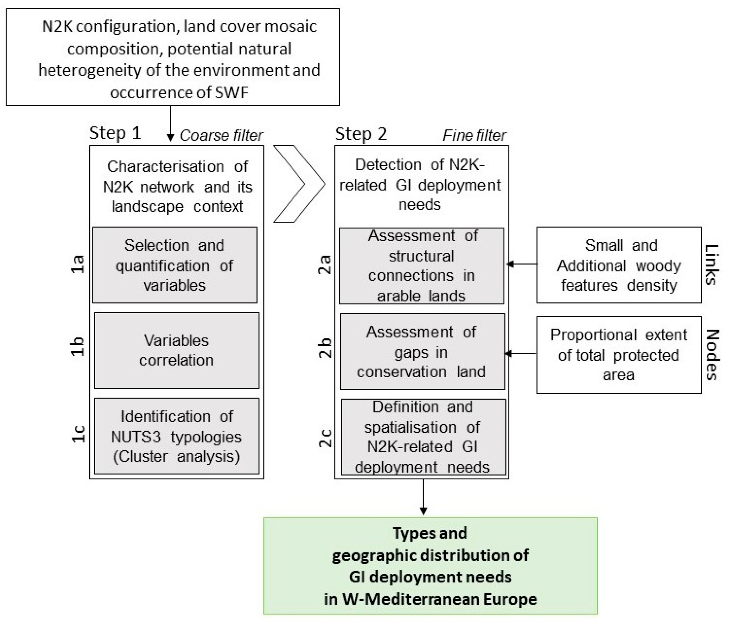
2.2. Research Design

This research was focused on W Mediterranean Europe NUTS3 and divided into two main steps (Figure 2). In the first step, aimed at coarsely characterising the N2K network and its landscape context, a set of pertinent variables was first selected and quantified (step 1a) and then correlated (step 1b). Therefore, only non-redundant variables were adopted for identifying different typologies of NUTS3 by means of a cluster analysis (step 1c).

The second step, designed to detect specific GI deployment needs across the study area, was focused on finer NUTS3 conditions in terms of nodes and links. As regards links, existing structural connections were especially investigated in arable lands, i.e., the most widespread landscape component within which N2K sites are interspersed. Accordingly, the cover density of residual woody elements was used as a variable to describe the arable land structural condition and was subsequently related to the NUTS3 typologies arising from the previous cluster analysis (step 2a). As far as nodes are concerned, in order to identify any gaps in conservation lands, the N2K network was complemented with alternative systems of protected areas (PAs) and the extent of the total protected area subsequently assessed (step 2b). Finally, by combining the overall information on network conditions, including the landscape context status that emerged from step 1, the N2K-related GI deployment needs were generalised and spatialised for individual NUTS3 (step 2c).

2.3. Characterisation of N2K Network and Its Landscape Context at the NUTS3 Level (Step 1)

2.3.1. Selection and Quantification of Landscape-Ecological Variables (1a) and Respective Correlation (1b)

In order to characterise the N2K network and its landscape context at the NUTS3 level, a set of spatial variables was selected and then quantified in a GIS environment (ArcGis 10.5). The selected variables concern the current N2K configuration, actual land cover mosaic composition, potential natural heterogeneity of the environment and occurrence of SWF (i.e., woody linear hedges and tree rows along field boundaries, riparian and roadside vegetation, and scattered patches of woods and shrubs) (

Table 1. Adopted variables, quantified by NUTS3, grouped into four main typologies: Natura2000 (N2K) network, land cover, potential natural heterogeneity of the environment and Small Woody Features (SWF).

Variable	Description	Source
Natura2000 network
Number of patches	Number of N2K patches	Natura2000 network vector layer [40]
Mean area	Total N2K area divided by the number of patches in km2
Patch density	Number of N2K patches with respect to the total area of NUTS3 in km2
Area density	Total N2K area with respect to the total area of NUTS3 in %
Edge density	Total edge area of N2K patches divided by the total area of NUTS3 (km/km2)
Land Cover
Artificial surfaces (CLC_art)	Percentage of artificial surfaces (map code 1, CLC 1st level) with respect to the total area of NUTS3 in %	Corine Land Cover (CLC) (land cover statistics from the “Land cover and change accounts 2000–2018” dataset) [45]
Agricultural surfaces (CLC_agr)	Percentage of agricultural surfaces (map code 2, CLC 1st level) with respect to the total area of NUTS3 in %
Natural surfaces (CLC_nat)	Percentage of natural surfaces (map code 3, CLC 1st level) with respect to the total area of NUTS3 in %
Arable land surfaces (21-Arable land)	Percentage of arable land surfaces (map code 21, CLC 2nd level) with respect to the total area of NUTS3 in %
Potential natural heterogeneity of the environment
Litho-morphological diversity (LM_diversity)	Shannon diversity index of litho-morphologic types	LANMAP3 [41]
Phytoclimatic diversity (PME_diversity)	Shannon diversity index of phytoclimatic types	Phytoclimatic map of Europe [46]
Small Woody Features (SWF)
Small woody feature cover density (SWF_D)	Cover density of linear and patchy SWF in the overall NUTS3 in %	“Small Woody Features” High-Resolution Layer [47]
Additional woody feature cover density (AWF_D)	Cover density of AWF, woody features connected to a valid SWF and isolated features larger than 1500 m2 (or wider than 30 m, if linear and out of specific patches) in the overall NUTS3 in %	“Small woody features” High-Resolution Layer [47]

).

To comprehensively consider the N2K network, contiguous and overlapping SCIs and SPAs were merged into unique patches and thus filtered according to a minimum threshold of 1 km².

The selected variables concerning the N2K extent and spatial configuration, including the number of patches, mean area, patch density, area density and edge density, were calculated with the Patch Analyst plugin (patch, size and edge metrics) [48].

Land cover variables, which are useful for characterising the landscape mosaic that hosts the N2K network in each NUTS3, include the proportional extent of artificial (CLC_art), agricultural (CLC_agr) and natural surfaces (CLC_nat, including wetlands and water bodies, besides forests and semi-natural areas), together with the proportional extent of arable land at a finer level of detail (21-Arable land), and were obtained from the CLC dataset provided by the European Environment Agency (land cover statistics from the “Land cover and change accounts 2000–2018” dataset) [45]. Among the second-level agricultural area types, which also include permanent crops, pastures and heterogeneous areas, arable lands were particularly investigated because they represent the most widespread land use type in the bioregion, often intensively managed, and therefore potentially affecting natural habitats’ persistence and connection more than the other agricultural surfaces [16,49,50,51].

Together with the actual landscape mosaic, biophysical variables were considered in order to characterise the NUTS3 in terms of the potential natural heterogeneity of the environment, which could, in turn, affect the consistency and condition of the N2K network. Combined parent material and morphological information were derived from LANMAP3 [41], with 33 litho-morphological classes occurring in the study area. Phytoclimatic information was derived from the phytoclimatic map of Europe (PME) [46], grouped into 50 types, 39 of which fall into the study area. For both litho-morphology and phytoclimate features, the NUTS3 environmental heterogeneity (LM_diversity and PME_diversity variables) was measured by means of the Shannon H index [52] based on the proportional extents of the classes [53].

SWF variables were selected due to the importance of small woody elements as (semi-) natural ecological links across highly fragmented landscapes [16,54,55]. Basic information on these features was retrieved from the raster layers of the Copernicus High-Resolution Layer product [47] at a resolution of 100 m, as recommended for large-scale landscape analyses [56]. Accordingly, the SWF density (SWF_D variable) and SWF + additional woody feature (AWF) density (SWF/AWF_D variable) were calculated for each NUTS3 with the ArcGis Zonal Statistics tool.

Thus, a correlation matrix was calculated using the Python 3.8.0 programming language (Python Software Foundation, 2022) to identify any redundant information among the selected variables listed in Table 1. Kendall Tau-b statistics [57] were employed for this purpose.

2.3.2. Identification of NUTS3 Typologies (1c)

In order to identify different NUTS3 typologies according to the selected variables, a K-medoids cluster analysis (default algorithm) was conducted with the Python package sklearn_extra.cluster.Kmedoids of scikit-learn. To avoid redundant information, one variable was excluded from clustering for each pair of significantly correlated variables with a correlation coefficient >+0.5 or <−0.5 [58,59]. Although non-linear models are not influenced by collinearity, excluding redundancies could prevent certain information from having greater weight than others [60].

K-medoids is a partitioning method of clustering n items into k clusters and is less sensitive to noise and outliers than the more commonly adopted K-means approach. Since the number of clusters (NC) should be chosen a priori, internal validation was undertaken in order to determine the optimal value [61]. Namely, for an NC ranging from 3 to 6, internal validation was carried out by means of the Silhouette coefficient and the Calinski–Harabasz criterion [62,63].

The Silhouette coefficient (S) ranges between −1 and +1 and scores the distances of each data point from its cluster and neighbouring clusters; it is calculated as:

$$S(i)=\frac{b\left(i\right)-a\left(i\right)}{max\left(b\right(i),a(i\left)\right)}$$

(1)

where a(i) is the average dissimilarity of i to all other data objects within the same cluster, and b(i) is the lowest average dissimilarity of i to any other cluster of which i is not a member.

A larger average Silhouette coefficient score indicates the better overall quality of the clustering result, showing either no substantial (below 0.25), weak (between 0.26 and 0.50), reasonable (0.51–0.70) or strong (more than 0.71) clustering structure [64,65].

The Calinski–Harabasz criterion (C) is a variance measure ratio of the within-cluster homogeneity and between-cluster heterogeneity [66]. It can be calculated as:

$$C=\frac{BGSS(N-K)}{WGSS(K-1)}$$

(2)

where WGSS is the sum of the within-cluster dispersions for all the clusters, and BGSS is the between-group dispersion. Its maximum average value determines the optimal NC [67].

Owing to its usefulness in outlier detection, the Silhouette coefficient has also been used to remove noisy observations and improve clustering performance [68]. Once the optimal NC was identified, observations with a negative Silhouette coefficient value were removed, and the algorithm was rerun.

Finally, the obtained and improved optimal NC was interpreted by means of a box plot and profile plot (the latter, for each n variable, was calculated as the ratio of the mean of the variable n in the k cluster to the overall mean of the same variable).

2.4. Detection of N2K-Related GI Deployment Needs (Step 2)

2.4.1. Links—Assessment of Existing Structural Connections in Arable Lands and Respective Relationships with Detected NUTS3 Typologies (2a)

In order to assess the existing structural connections in arable lands, which can be considered a proxy for the condition of this land cover type with respect to the ecological connectivity capacity [69], the density of existing natural and semi-natural landscape elements was quantified. For this purpose, two variables were measured: the proportional extent of arable land by NUTS3, retrieved from the national CLC vector layer [70], and the SWF + AWF (SAWF) cover density, derived from the respective 100 m raster layer. The latter was quantified by means of the Zonal Statistics tool for the arable land of each NUTS3 and then grouped into five classes according to quantiles.

To check the calculation accuracy, SAWF cover density measures were repeated in 8 randomly chosen NUTS3 based on the SWF vector layer (which includes linear, patchy and AWF classes) [47].

SAWF cover density values were then correlated with the proportional extent of arable land by means of the Spearman correlation coefficient [71] in XLSTAT 2022.2.1 software (Addinsoft, 2022). The level of significance was set at p ≤ 0.05.

Finally, in order to assess the relationships between arable land with different conservation statuses and the previously detected typologies of NUTS3, (i) the SAWF cover density quantiles were converted into categorical classes, (ii) the frequencies of these categorical classes were quantified for each cluster, and (iii) the significance of frequency differences among the clusters was assessed. Specifically, a Chi-square test was carried out [72], while the significance by cell and the strength of the association were assessed by means of Fisher’s exact test [73] and Cramer’s V statistics [74], respectively.

2.4.2. Nodes—Assessment of Gaps in Conservation Lands (2b)

In order to identify any gaps in terms of protected area coverage, the contribution of alternative systems of PAs with respect to N2K was considered. Namely, the layers of the national systems of PAs [75,76,77,78] were superimposed on the N2K network, and, for each NUTS3, the proportional extent of the total protected area was assessed.

A threshold of 10% was adopted as the minimum conservation target, where a smaller protected surface is considered a gap in the network system [79,80].

2.4.3. Definition and Spatialisation of N2K-Related GI Deployment Needs (2c)

Finally, to define the N2K-related GI deployment needs, the information arising from the evaluation of the specific conditions in terms of nodes and links was combined with the NUTS3 typologies (diagnostic of the coarser landscape context status) identified with the first research step. Thus, the detected GI deployment needs were described, hierarchically arranged (by giving more importance to node gaps over the deficit of links) and geographically represented.

3. Results

3.1. Landscape-Ecological Features of W Mediterranean Europe NUTS3 (Step 1)

3.1.1. Variable Quantification (1a)

The distribution of the 13 selected variables values in the analysed NUTS3, grouped by country (Spain, France, Italy and Portugal) and by typology (N2K, land cover, potential natural heterogeneity of the environment, and SWF), is summarised in Figure 3.

As regards N2K variables, the Mediterranean NUTS3 in Spain and France have a higher number of patches (33.47 and 33.76 mean values, respectively) than those in Italy and Portugal (19.80 and 6.85, respectively). The mean area of N2K patches is higher in Spain and Portugal (104.20 and 126.65 km², respectively) than in France and Italy (39.50 and 31.60 km², respectively), while the patch density is higher in France and Italy (0.65 and 0.82, respectively) than in the Iberian Peninsula (0.38 in Spain and 0.17 in Portugal). The edge density is very similar in Spain (0.22), France (0.24) and Italy (0.22), while it has a lower value in Portugal (0.09). Finally, the area density decreases from Spain (25.90%) to Portugal (15.80%) via France (22.66%) and Italy (18.29%), and it is the only variable without outliers.

As regards land cover variables, the Mediterranean NUTS3 in France and Italy show the highest mean values of artificial surfaces (6.00 and 5.00%, respectively); those in Spain and Italy have the highest values of agricultural surfaces (48.00 and 54.00%), especially arable lands; and those in France and Portugal have the highest values of natural areas (67.00 and 56.00%). Outliers were especially found in the distribution of artificial and arable land surfaces in Italy.

As regards the potential natural heterogeneity of the environment, the Mediterranean NUTS3 in Portugal have the lowest mean values for both litho-morphological (0.81) and phytoclimatic (0.74) diversity, but, overall, there are no marked differences between countries, and no outliers were identified.

Finally, both SWF variables have higher mean values in France and Portugal than in Spain and Italy. The mean SWF density values, for example, are equal to 4.09 and 2.28% for the former and 1.72 and 1.60% for the latter. Outliers occur for both variables, except for in France.

3.1.2. Correlation between Variables (1b)

Correlations between the selected variables are summarised in Figure 4. The strongest correlations, with a coefficient > +0.5 or <−0.5, emerged between the following pairs of variables: “Area density” and “Number of patches”; “Patch density” and “Mean area”; CLC_nat and CLC_agr; SWF_D and SWF/AWF_D; and CLC_nat and 21-Arable land. Accordingly, “Number of patches”, “Patch density”, “Edge density”, CLC_art, CLC_agr, 21-Arable land, SWF_D, LM_diversity and PME_diversity were retained for the following cluster analysis, while “Area density”, “Mean area”, CLC_nat and SWF/AWF_D were excluded.

3.1.3. Characteristic Features and Geographic Distribution of NUTS3 Clusters (1c)

According to the average Silhouette (0.494) and Calinski–Harabasz (234.385) scores, four NCs were considered (

Table 2. Average Silhouette and Calinski–Harabasz scores for numbers of clusters (NC) ranging from 3 to 6.

NC	Average Silhouette Score	Average Calinski–Harabasz Score
3	0.439	148.833
4	0.494	234.285
5	0.458	233.141
6	0.416	217.662

).

A total of 25 NUTS3 belong to cluster 1 (K1), 39 belong to cluster 2 (K2), 37 belong to cluster 3 (K3) and 28 belong to cluster 4 (K4). Seven outliers were identified and then removed, six from K1 (with a final total of nineteen NUTS3) and one from cluster K2 (with a final total of thirty-eight NUTS3). After their removal and algorithm reprocessing, the clustering performance improved, with an average Silhouette score that increased to 0.531, reaching a valid reasonable clustering structure [62,63], and an average Calinski–Harabasz score that increased to 275.797.

The profile plot of the variables included in the four clusters is shown in Figure 5.

On average, the NUTS3 belonging to the different clusters are characterised by (

Table 3. Mean and standard error of the mean values for each of the 8 selected variables by cluster (“Number of patches” (NP); “Patch density” (PD); CLC_art, percentage of artificial surfaces; CLC_agr, percentage of agricultural surfaces; SWF_D, density of small woody elements; “Edge density” (ED); LM_diversity, litho-morphological diversity; PME_diversity, phytoclimatic diversity; 21-Arable land, percentage of arable surfaces).

K	NP	PD	CLC_art	CLC_agr	SWF_D	ED	LM_Diversity	PME_Diversity	21-Arable Land
1	51.800 $\pm$2.700	0.630 $\pm$0.100	0.037 $\pm$0.001	0.540 $\pm$0.040	1.930 $\pm$0.400	0.230 $\pm$0.020	1.270 $\pm$0.080	0.940 $\pm$0.100	0.290 $\pm$0.040
2	28.280 $\pm$0.600	0.730 $\pm$0.100	0.052 $\pm$0.009	0.440 $\pm$0.030	2.210 $\pm$0.250	0.250 $\pm$0.020	1.340 $\pm$0.050	1.240 $\pm$0.070	0.190 $\pm$0.020
3	15.650 $\pm$0.500	0.510 $\pm$0.050	0.046 $\pm$0.007	0.520 $\pm$0.030	1.780 $\pm$0.200	0.190 $\pm$0.015	1.160 $\pm$0.060	0.950 $\pm$0.070	0.220 $\pm$0.026
4	5.860 $\pm$0.500	0.330 $\pm$0.060	0.048 $\pm$0.007	0.450 $\pm$0.030	2.050 $\pm$0.220	0.150 $\pm$0.020	0.850 $\pm$0.100	0.800 $\pm$0.070	0.110 $\pm$0.017

Values are conditionally formatted to highlight the variation in variable means among clusters (from lowest values in white to highest values in dark green).

):

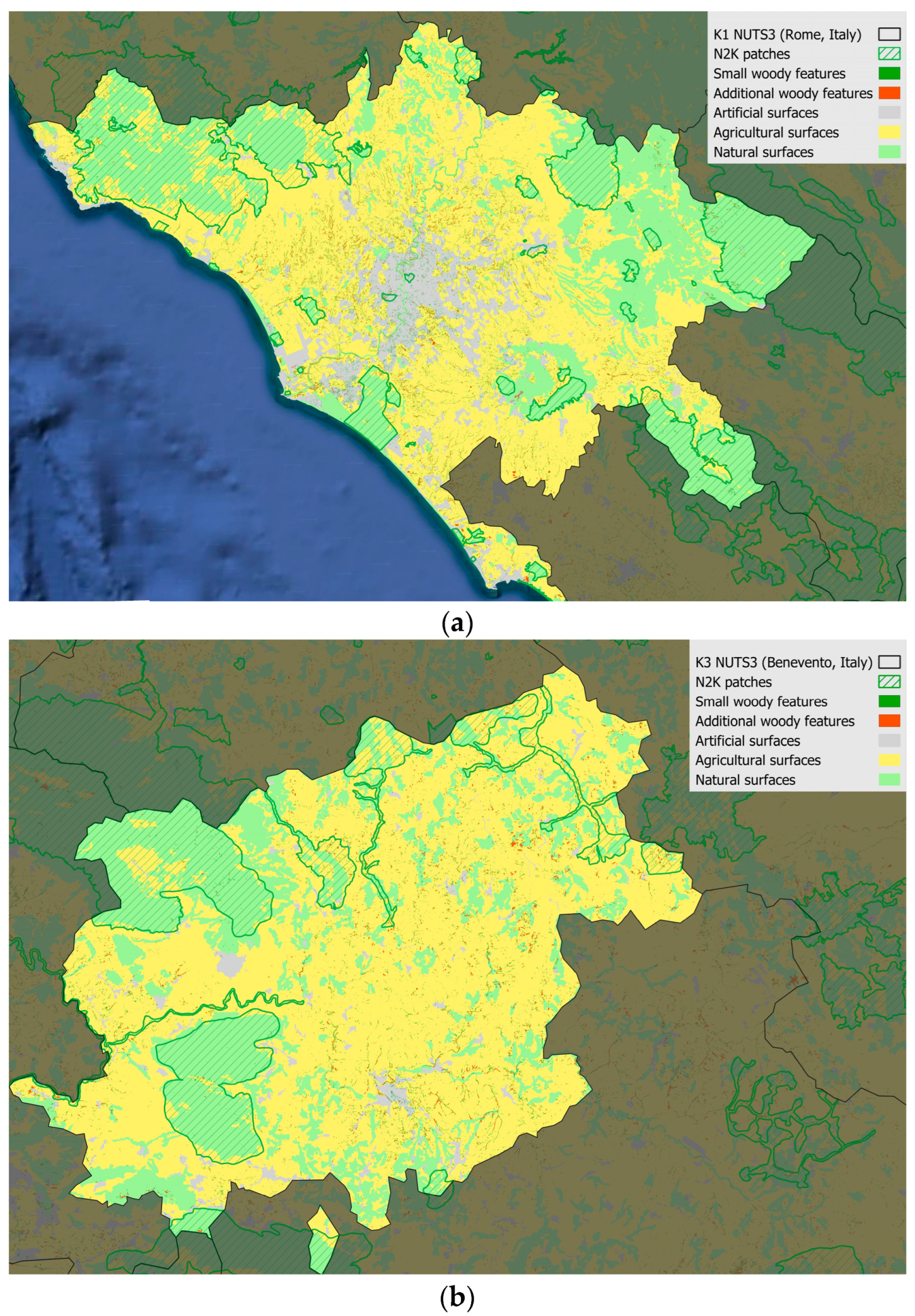
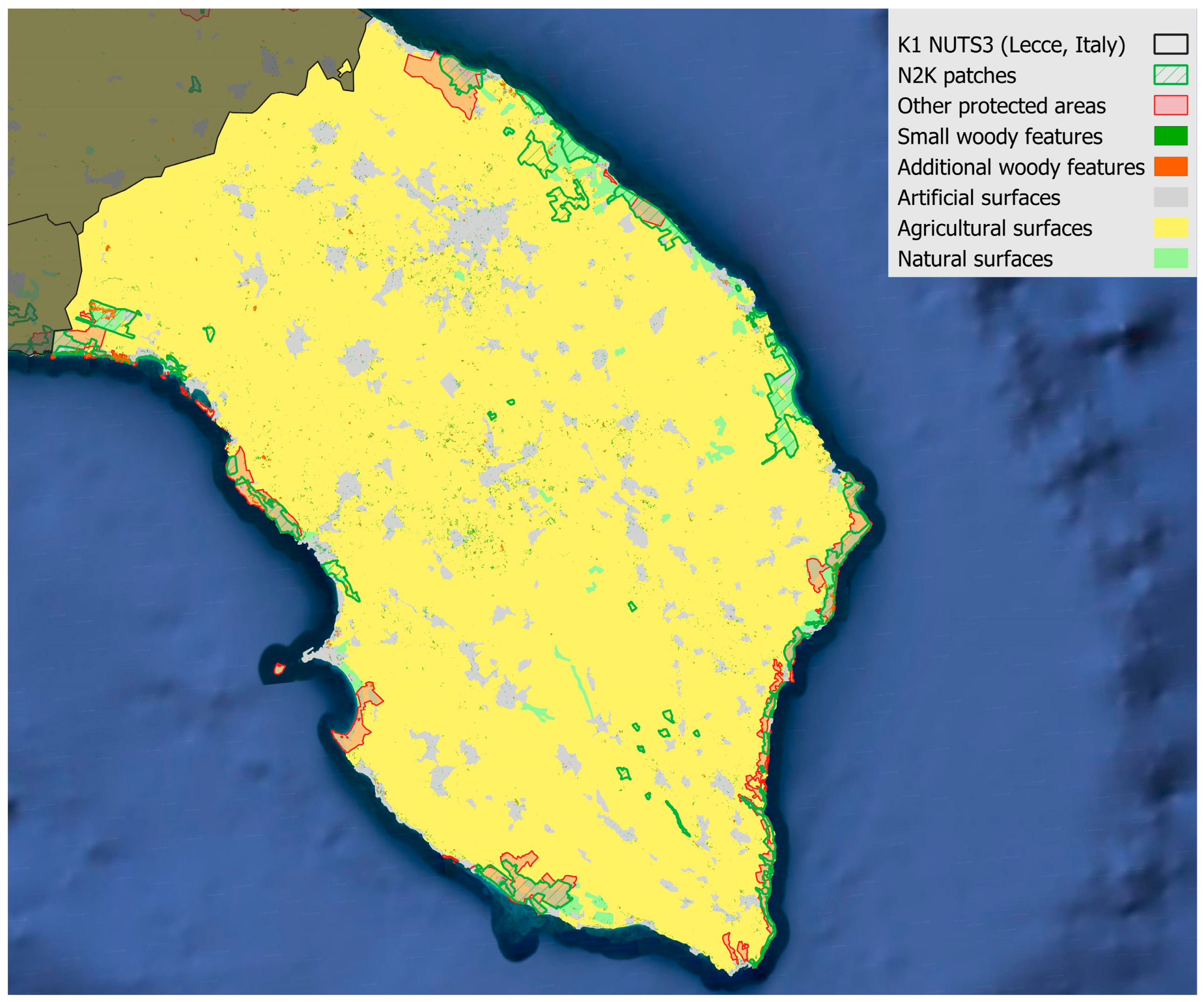
• K1—a high number of N2K patches, although not with the highest density, interspersed in agricultural matrices with a medium-low SWF density;
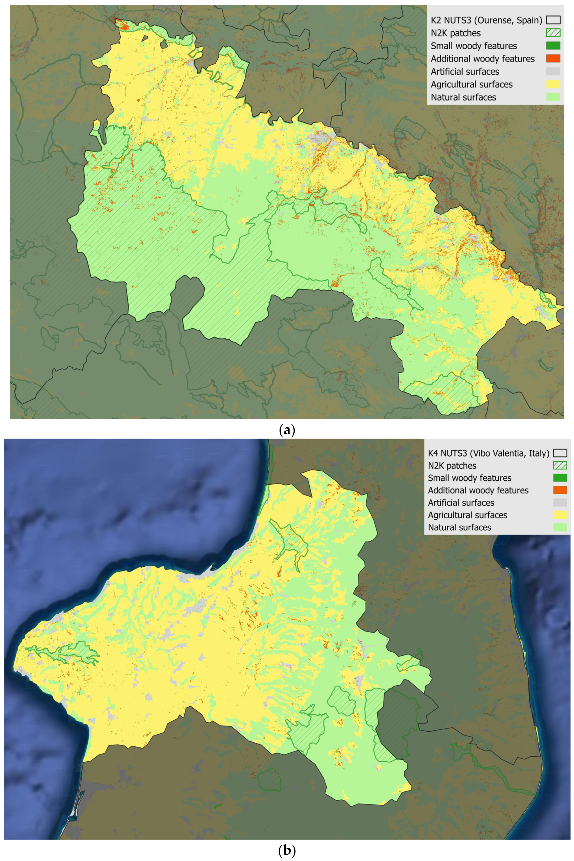
• K2—a medium-high number of N2K patches, with the highest density of patches and edges, interspersed in natural matrices with the highest SWF density and the highest litho-morphological and phytoclimatic diversity;
• K3—a medium-low number of N2K patches, with a medium-low density, interspersed in agricultural matrices with the lowest SWF density;
• K4—a small number of N2K patches, which also have the lowest density, interspersed in natural matrices with a high SWF density but low environmental heterogeneity.

Overall, according to the between-group variance, the number of N2K patches is the most discriminating variable between clusters (Figure 6). Apart from this feature, NUTS3 belonging to K1 and K3 share a more rural landscape character, with the dominance of arable lands and scattered SWF, while those belonging to K2 and K4 show a more natural landscape character with dense SWF.

In terms of geographic distribution (map provided in Appendix A), NUTS3 belonging to K1 are predominantly located in Mediterranean Spain, especially in inland sectors; NUTS3 belonging to K2 are predominantly located in mountain or high-hill sectors in Mediterranean France, where this type is the most widespread, Spain and Italy; NUTS3 belonging to K3 are mainly located in Italy; and those belonging to K4 prevail in Portugal, as well as in coastal Italy and insular Spain.

3.2. N2K-Related GI Deployment Needs in W Mediterranean Europe (Step 2)

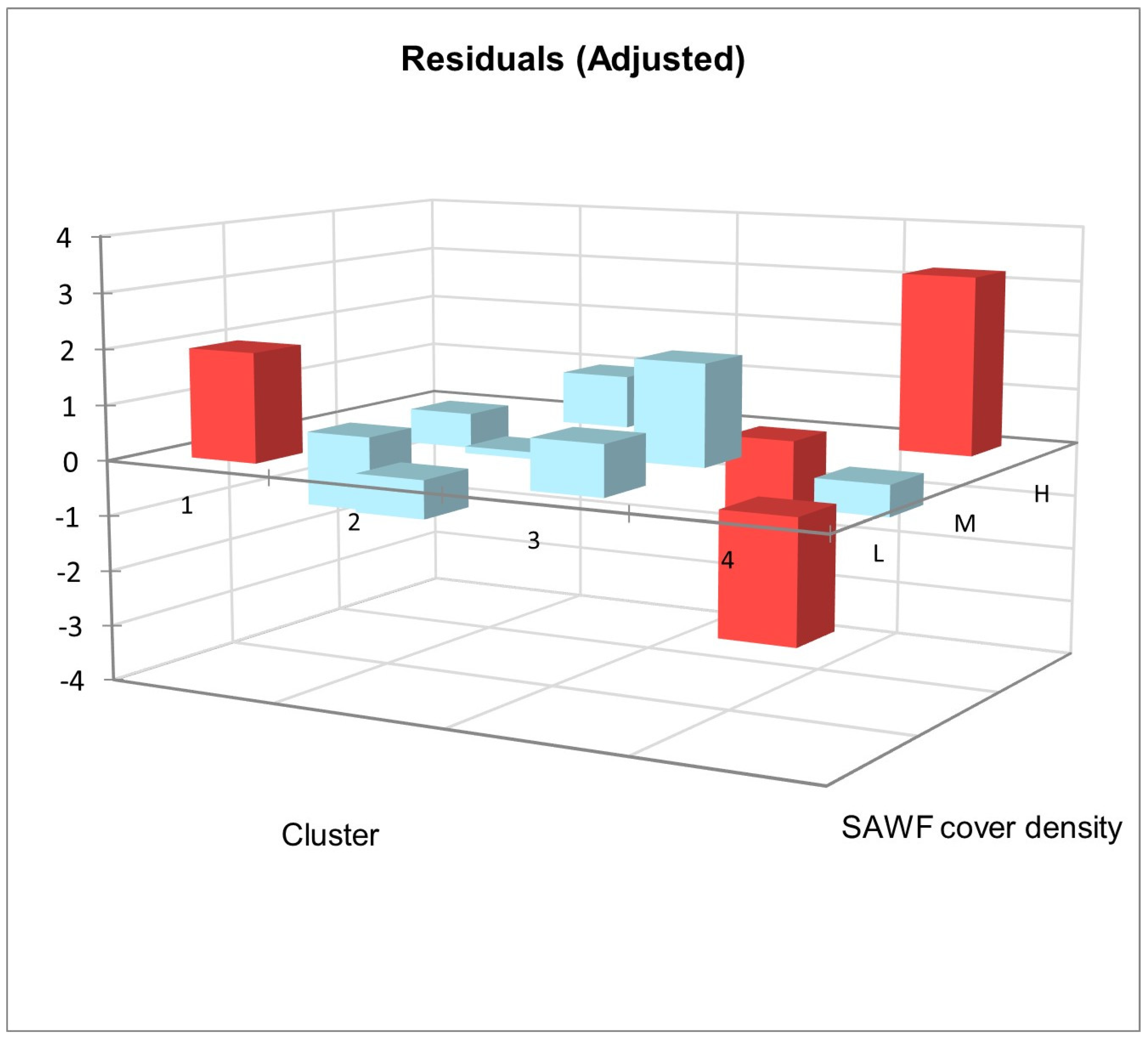
3.2.1. Structural Conditions of Arable Lands and Respective Relationship with the Detected NUTS3 Typologies (2a)

The SAWF cover density within arable lands in each of the 129 NUTS3 under study, grouped by quantiles, is shown in Figure 7. The higher the SAWF cover density, the better the considered arable land structural condition.

The density of residual natural elements in arable lands is higher than 10% (i.e., the percentage of agricultural area that should be converted to high-biodiversity landscape features according to the EU Biodiversity Strategy target) in just 13 NUTS3 out of the total. These NUTS3 are mostly located in northern Portugal and Mediterranean France, and 7 out of these 13 are characterised by a low proportional extent of arable lands (<5%—see Appendix B).

As regards the correlation between variables, Spearman statistics showed a significant negative association between the SAWF cover density and the proportional extent of arable land (coefficient = −0.55; p < 0.0001), suggesting that sizeable arable lands are likely to be characterised by intensive cultural practices that caused the disappearance of such landscape elements.

The verification of the SAWF cover density calculation shows that the density value calculated from the raster layer differs on average by $\pm \overline{0.1}$ from that calculated from the vector layer for the eight randomly selected NUTS3. Therefore, the calculation conducted on the basis of the raster was considered reliable.

The structural conditions assigned to arable lands, according to the categorical classes of the SAWF cover density, are shown in

Table 4. Classes of structural conditions assigned to arable lands according to SAWF cover density.

Quantile Class	Range (%)	SAWF Density Categorical Class	Arable Land Structural Condition
1st and 2nd	0–3	Low (L)	Unfavourable
3rd and 4th	3.1–6.5	Medium (M)	Adequate
5th	6.6–18.7	High (H)	Favourable

, while the frequencies of such classes in the four NUTS3 typologies are shown in Figure 8.

The test for independence highlights significant differences in the frequencies of SAWF cover density between clusters (Chi-square value = 20.2; p = 0.003). The significance by cell (Fisher’s exact test, p = 0.001) shows, in particular, the contribution of each value to the overall significance of the Chi-square test: the high frequencies of class H in K4, the low frequencies of the same class in K3 and the low frequencies of class L in K4 have the most significant values (p = 0.004, 0.001 and 0.047, respectively). According to the analysis of residuals (Figure 9), the high frequency of class L in K1 is significant as well (p < 0.05).

The overall strength of the association, assessed by Cramer’s V statistic, is equal to 0.280, which indicates a medium-intensity dependence between the variables [81].

These outcomes highlight the expected link between the clustering structure and the structural conditions of arable land and, especially considering the different behaviour of class H with respect to class L, suggest the potential role of arable land conditions in detecting N2K-related GI deployment needs. Namely, when under unfavourable conditions, arable lands are likely to behave as ecological barriers due to the low SAWF cover density, whereas, under favourable conditions, they could function as a permeable matrix due to the higher density of connecting elements (e.g., for woody plant dispersal [16]) (Figure 10).

Furthermore, in order to avoid an under- or overestimation of the potential barrier effect of arable lands, an unfavourable condition was assumed a priori for arable lands covering more than 33% (fifth extent quantile) of the respective NUTS3, while a favourable condition was assumed a priori for arable lands covering less than 5% of the respective NUTS3 (first extent quantile).

3.2.2. Total Protected Area by NUTS3 (2b)

The assessment of total conservation lands resulted in the identification of 14 NUTS with less than 10% of PAs (N2K + national PAs). Seven out of these fourteen belong to K4, where this deficiency is due to the small number of N2K patches that characterises the group. On the other hand, six belong to K3 and one belongs to K1, where the gap is due to the small sizes of protected sites (average area < 16 km²), although numerous, and to the frequent overlaps between the different protection systems.

3.2.3. General N2K-Related GI Deployment Needs (2c)

On the basis of the previous results, four different GI deployment needs were generalised for individual NUTS3 of the W Mediterranean EU: (a) the need for consolidating node and link conservation, (b) the need for connection restoration, (c) the need for the creation of new protected sites and (d) the need for N2K site enlargement.

Priority was given to gaps in conservation lands rather than those in potential connections between protected sites so that precedence was given to conditions in terms of nodes rather than links for the definition of prevalent GI needs. For NUTS3 with needs (a) and (b), no gaps were identified in conservation land.

(a)

Need for consolidating node and link conservation

The detected need for consolidating node and link conservation involves GI deployment aimed at strengthening efforts to conserve existing network components, which include both the habitat nodes already protected and the existing links that might benefit from more diffuse conservation measures. Overall, NUTS3 with conservation reinforcement needs, predominantly assigned within K2 and K4, show high natural cover ($\overline{0.580}\pm 0.022$%) coupled with a high average cover density of SWF/SAWFs (in total or in arable land only), which suggests the actual occurrence of an effective ecological network (Figure 11).

According to the assessed occurrence of structural links, these needs were assigned to all NUTS3 where the resulting arable land conditions are favourable or, alternatively, to NUTS3 in K2 and K4 (characterised by a low proportional extent of agricultural land combined with a relatively high SWF density) when the resulting arable land conditions are adequate.

(b)

Need for connection restoration

The detected need for connection restoration refers to GI deployment aimed at an improvement in the N2K network by placing additional (semi-)natural elements across the landscape matrix, with a focus on the dominant agricultural matrix and with expected benefits for both protected habitats and crop productivity.

Overall, NUTS3 with this need, predominantly assigned within K1 and K3, show little residual natural cover ($\overline{0.390}\pm 0.019$%) coupled with a low cover density of SWF/SAWFs (in total or in arable land only), which may mean a lack of GI components potentially acting as ecological links (Figure 12).

According to the current structural link occurrence, these needs were assigned to all NUTS3 where the resulting arable land conditions are unfavourable or, alternatively, to NUTS3 in K1 and K3 (characterised by a high proportional extent of agricultural land combined with a relatively low patch and overall SWF density) when the resulting arable land conditions are adequate.

(c)

Need for the creation of new protected sites

Due to a lack of an adequate proportion of protected natural areas, the need for the creation of new protected sites was detected in NUTS3 characterised by few N2K patches, despite the high coverage of natural habitat (i.e., those in K4), and with a proportional extent of the total protected area below the critical threshold of 10%. For these NUTS3, the establishment of new protected areas may be a feasible intervention due to the availability of natural habitats and may easily allow the minimum conservation target to be reached (Figure 13).

(d)

Need for N2K site enlargement

Still in terms of the 10% total protected area threshold, similar criticalities were found in NUTS3 with a higher coverage of agricultural lands (i.e., those in K1 or K3). In this case, the scarce availability of natural habitats prevents the establishment of new protected areas. As a result, and also considering the extremely small size of N2K areas (average area < 16 km²), the need for N2K site enlargement was recognised. To mitigate pressures from widespread agricultural practices, this action could also be implemented by defining buffer zones around N2K patches in which to promote restoration interventions and climate change adaptation practices (Figure 14).

The geographic distribution of the detected N2K-related GI deployment needs is shown in Figure 15.

Overall, the prevailing need for consolidating node and link conservation was identified for 52 NUTS3 (40%), primarily belonging to K2 and K4, which dominate Mediterranean Portugal and France and are widespread in the mountain and high-hill sectors of Spain and Italy. The prevailing need for connection restoration was identified for 63 NUTS3, which is about 49% of the total, mainly located in Mediterranean Spain and Italy and belonging to K1 and K3. The need for the creation of new protected sites, identified for seven NUTS3 (5.5%), prevails in Portugal and is located exclusively in K4 NUTS3. Lastly, the need for N2K site enlargement was identified for seven NUTS3 (5.5%) and is exclusive of Mediterranean Italy, mostly in the south and in K3 NUTS3.

According to the share of NUTS3 types for each GI deployment need (

Table 5. Number of NUTS3 with specific GI deployment needs per cluster (NUTS3 type).

		GI Needs
		Consolidating Node and Link Conservation	Connection Restoration	N2K Site Enlargement	New Protected Site Creation
Cluster	K1	5	19	1	0
	K2	22	17	0	0
	K3	8	22	6	1
	K4	17	5	0	6
	Total	52	63	7	7

), the cluster/need relationships are graphically represented in the radar plot in Figure 16.

The official NUTS3 codes, with the respective clusters to which they belong and the recognised GI deployment needs, are listed in Appendix C.

4. Discussion

To define the type and distribution of N2K-related GI deployment needs in W Mediterranean Europe, a multistep process was developed, which was divided into coarse- and fine-filter analyses, in line with previous research approaches [82,83,84].

By means of this preliminary wide-scale investigation, four different types of GI deployment needs were recognised and generalised at the NUTS3 level, which may facilitate the selection of priority areas in which to intervene for an effective improvement in the N2K network [9,85] before designing tailored actions at more local scales.

Following the identification of a number of contiguous NUTS3 with the same need, it also becomes possible to facilitate the selection of macro-areas for the construction or formalisation of a Trans-European Nature Network (TENN) [6,8]. For example, most of the detected needs are for connection restoration, and several neighbouring NUTS3 with this same requirement could lead to the selection of priority trans-country pathways (e.g., across contiguous NUTS3 in Spain and Portugal) [86]. On the other hand, the high conservation value of Mediterranean France and of the Italian Ligurian coasts has the potential to serve as an ecological corridor between the more anthropised NUTS3 in the rest of peninsular Italy and Spain, especially considering the good number of primary forests (i.e., forests having a high naturalness) still remaining in the sector [87,88].

Furthermore, our findings support the evidence that land biophysical features frequently predispose the area to different structural and functional ecological network conditions [16,89], which should prompt the combination of different intervention strategies based on the initially identified “ecological performance” [90]. For example, conservation reinforcement needs, as well as most of the protected areas, are mostly found in mountain or high-hill sectors, where the lack or abandonment of agricultural practices may have contributed less to habitat fragmentation [91,92]. On the contrary, most of the need for connection restoration is found in NUTS3 with abundant plain or low-hill areas, confirming the morphological predisposition of these sectors to the development of pervasive agricultural practices [22,23,24] and to urbanisation [93]. This result is certainly influenced by the adopted criteria but stresses the need to also consider the difference between the actual and potential cover of natural ecosystems during the prioritisation process [94]. In fact, as previously observed at more local scales [16], focusing directly on the spatial patterns of remaining habitats resulted in some sectors being ranked with a low priority in terms of reconnection, but only because they actually lack adequate natural cover.

Overall, the investigation was useful in understanding the N2K network GI deployment needs and how these are distributed across W Mediterranean Europe but is likely to be insufficient to suggest locally tailored GI conservation and restoration actions. In fact, a clear understanding of the complexity of the current ecological network, the assessment of ecological connection gaps [95] and the identification of specific priority sites to be preserved require finer spatial and thematic scales of analyses [96].

Taking this limitation into account, the detected need for consolidating node and link conservation allowed a NUTS3 group with potentially adequate N2K patch coverage and connectivity to be identified. In these NUTS3, more detailed conservation status assessments [94,97] and the identification of important biodiversity areas [98,99,100] should therefore be performed at the local scale to identify and prioritise specific conservation actions. Moreover, the fragmenting effect of artificial surfaces should be considered, besides that of agricultural land, especially for those NUTS3 with widespread urban areas (e.g., Naples and Caserta NUTS3 in Italy) [101].

The detected need for connection restoration highlights a group of NUTS3 that are potentially critical in terms of ecological connectivity. However, the identification of patches for effective reconnection requires the habitats and species occurring in N2K sites to be explicitly considered [102], intra- and inter-site fragmentation to be assessed [103], and structural and functional connectivity to be measured [16,100]. Since connectivity, especially in functional terms, is a species-specific landscape attribute [104], only studies that consider the specific needs of animal and plant organisms can propose coherent and targeted intervention strategies. In this case, due to the spatial extent of the study area, fine-scale connectivity analyses would have taken excessively long and would have gone beyond the aims of a preliminary investigation.

On the other hand, the detected need for the creation of new protected sites characterises a NUTS3 group lacking an adequate proportion of protected natural surfaces, i.e., below the critical 10% coverage threshold [79,80]. In order to maintain adequate biodiversity protection, each country is actually required by the international Convention on Biological Diversity to protect at least 10% of its total land area [105]. Even so, we demonstrate that several NUTS3 in W Mediterranean Europe (i) fail to achieve this minimum level of nature protection and (ii) are far from the target of protecting 30% of the land by 2030 set by the EU Biodiversity Strategy [10]. Not surprisingly, these gaps were found especially in Portugal where, along with Cyprus, Malta, Luxembourg and the Netherlands, terrestrial protected areas are very few in number (<500) and have a proportional extent lower than the EU average (22 vs. 28%, respectively) [106].

Likewise, the detected need for N2K site enlargement highlights NUTS3 with a total protected area of less than 10% but combined with typically small N2K patches (average area < 16 km²) that are mostly interspersed in a homogeneous agricultural matrix. As a result of the reduced presence of residual natural habitats, site enlargement may be better pursued in these cases, for example, by creating a buffer zone to mitigate the pressure from agricultural practices. The negative impact of the urbanisation and intensification of agricultural activity close to N2K sites has already been highlighted, but clear EU legislation on eligible land uses in N2K buffer areas is lacking and thus not preventing the loss of supporting ecosystems services provided by the network [107]. There is therefore a particular need to define and regulate when and how to incorporate buffer areas for enhancing the functionality of N2K sites.

This preliminary wide-scale investigation also allowed the structural condition of arable land in the W Mediterranean Europe to be assessed. According to the latest EU guidelines on ecosystem condition assessment [69], the arable land structural status was evaluated through the quantification of the SAWF cover density. As far as is known, this assessment is the first of its kind, offers a quite easy and fast calculation method even for very large areas and may contribute to achieving the target of converting at least 10% of agricultural areas to high-diversity landscape features [10]. The implementation of this last action actually emerged as a priority in W Mediterranean Europe NUTS3, considering that (i) despite the lack of comparison with other biogeographical regions, only 13 out of the 129 investigated NUTS3 (about 10%) have an SWF cover density above the EU target threshold, and (ii) the extent of arable land is inversely correlated with the SAWF cover density in NUTS3. Although predictive models would have provided more precise information on potential causality, these findings confirm the evidence that agriculture intensity represents a major cause of the loss of natural landscape elements [31,32,33,34] and suggest that the greater the arable land area, the more restoration actions required.

Despite these valuable insights, some considerations should be made about the methodology, especially as regards the adopted basic data. First, the available SWF layer [47] does not include the elements falling under permanent crops, even though these agricultural areas may represent an important “refuge” for biodiversity [108,109]. Second, accounting for only 30% of the total landscape features, SWF are not the only natural factor characterising “diffuse naturalness” in agricultural settings [18,67]. However, taking other small landscape features into account besides woody ones could result in unrealistic assessments of agroecosystem conditions. The very intensive agricultural matrix of the Po Valley in north-east Italy, for example, was found to have one of the highest densities of linear landscape elements in Europe due to grass ditches, despite the very poor conservation status of all the existing ecosystems and of the overall ecoregion [110,111].

Third, although the degree of naturalness affects their capacity to provide ecosystem services [112,113], the mapped SWF are not distinguished in terms of quality, e.g., according to the share of native plant species [16,114,115]. The present investigation should therefore be complemented with a finer SWF condition assessment, and, in general, the need to harmonise the understanding of the definition and type of these residual landscape features at the EU level has been confirmed [116].

5. Conclusions

This wide-scale preliminary investigation served as an initial filter to select priority areas for the effective improvement of the EU N2K network before intervening with tailored actions at the local level. Since the criteria for selecting these areas are usually comprised of various contrasting factors, our results could guide, with scientific backing, some of the choices regarding W Mediterranean Europe. The four detected GI deployment needs summarise the current status of the N2K network and highlight its main vulnerabilities, while the representation of their geographical distribution will allow these needs to be integrated into broader and more ambitious conservation strategies. This research also emphasised the role of agricultural land in preventing or promoting the structural coherence of the N2K network, as well as the relevance of small woody features in defining the conditions of this landscape component. Lastly, although useful for a preliminary GI priority setting and despite their high spatial resolution, the shortcomings related to European-level data were highlighted with respect to truly effective actions to be designed at more detailed scales.

References

1. Mézard, N.; Sundseth, K.; Wegefelt, S. Natura 2000: Protecting Europe’s Biodiversity; EC (European Commission), Directorate General for the Environment, Publications Office. 2008. Available online: https://data.europa.eu/doi/10.2779/23868 (accessed on 29 March 2023).
2. EC (European Commission). Natura 2000—Environment. 2022. Available online: https://ec.europa.eu/environment/nature/natura2000/index_en.htm#:~:text=Stretching%20over%2018%25%20of%20the,and%20threatened%20species%20and%20habitats (accessed on 29 March 2023).
3. EC (European Commission). Directive 2009/147/EC of the European Parliament and of the Council of 30 November 2009 on the Conservation of Wild Birds; Official Journal L 20, 26/01/2010, 7–25; European Commission: Brussels, Belgium, 2010. [Google Scholar]
4. EC (European Commission). Council Directive 92/43/EEC of 21 May 1992 on the Conservation of Natural Habitats and of Wild Fauna and Flora; Official Journal L 206, 22/07/1992, 7–50; European Commission: Brussels, Belgium, 1992. [Google Scholar]
5. Estreguil, C.; Caudullo, G.; de Rigo, D.; San-Miguel-Ayanz, J. Forest Landscape in Europe: Pattern, Fragmentation and Connectivity. Eur. Sci. Tech. Res. 2013, 25717, 18. [Google Scholar]
6. EEA (European Environment Agency). Contributions to Building a Coherent Trans-European Nature Network. 2020. Available online: https://www.eea.europa.eu/themes/biodiversity/green-infrastructure/building-a-coherent-trans-european/contributions-to-building-a-coherent/view (accessed on 29 March 2023).
7. Falcucci, A.; Maiorano, L.; Boitani, L. Changes in land-use/land-cover patterns in Italy and their implications for biodiversity conservation. Landsc. Ecol. 2007, 22, 617–631. [Google Scholar] [CrossRef]
8. EEA (European Environment Agency). Building a coherent Trans-European Nature Network. 2020. Available online: https://www.eea.europa.eu/publications/building-a-coherent-trans-european (accessed on 29 March 2023).
9. EC (European Commission). Criteria and Guidance for Protected Areas Designations—Staff Working Document. 2022. Available online: https://environment.ec.europa.eu/publications/criteria-and-guidance-protected-areas-designations-staff-working-document_en (accessed on 29 March 2023).
10. EC (European Commission). EU Biodiversity Strategy for 2030-Bringing Nature Back into Our Lives; Communication from the Commission to the European Parliament, the Council, the European Economic and Social Committee and the Committee of the Regions COM. 2020. Available online: https://eur-lex.europa.eu/legal-content/EN/TXT/?qid=1590574123338&uri=CELEX:52020DC0380 (accessed on 29 March 2023).
11. EC (European Commission). Communication from the Commission to the European Parliament, the Council, the European Economic and Social Committee and the Committee of the Regions. Green Infrastructure (GI)—Enhancing Europe’s Natural Capital. 2013. Available online: https://eur-lex.europa.eu/legal-content/EN/TXT/?uri=celex%3A52013DC0249 (accessed on 2 June 2023).
12. Honeck, E.; Moilanen, A.; Guinaudeau, B.; Wyler, N.; Schlaepfer, M.A.; Martin, P.; Sanguet, A.; Urbina, L.; von Arx, B.; Massy, J.; et al. Implementing Green Infrastructure for the Spatial Planning of Peri-Urban Areas in Geneva, Switzerland. Sustainability 2020, 12, 1387. [Google Scholar] [CrossRef] [Green Version]
13. Xia, H.; Ge, S.; Zhang, X.; Lei, Y.; Liu, Y. Spatiotemporal Dynamics of Green Infrastructure in an Agricultural Peri-Urban Area: A Case Study of Baisha District in Zhengzhou, China. Land 2021, 10, 801. [Google Scholar] [CrossRef]
14. Gómez-Villarino, M.T.; Gómez-Villarino, M.; Ruiz-Garcia, L. Implementation of Urban Green Infrastructures in Peri-Urban Areas: A Case Study of Climate Change Mitigation in Madrid. Agronomy 2021, 11, 31. [Google Scholar] [CrossRef]
15. Hanna, E.; Comín, F.A. Urban Green Infrastructure and Sustainable Development: A Review. Sustainability 2021, 13, 11498. [Google Scholar] [CrossRef]
16. Valeri, S.; Zavattero, L.; Capotorti, G. Ecological connectivity in agricultural green infrastructure: Suggested criteria for fine scale assessment and planning. Land 2021, 10, 807. [Google Scholar] [CrossRef]
17. Capotorti, G.; Alós Ortí, M.M.; Copiz, R.; Fusaro, L.; Mollo, B.; Salvatori, E.; Zavattero, L. Biodiversity and ecosystem services in urban green infrastructure planning: A case study from the metropolitan area of Rome (Italy). Urban For. Urban Green. 2019, 37, 87–96. [Google Scholar] [CrossRef]
18. Capotorti, G.; Valeri, S.; Giannini, A.; Minorenti, V.; Piarulli, M.; Audisio, P. On the Role of Natural and Induced Landscape Heterogeneity for the Support of Pollinators: A Green Infrastructure Perspective Applied in a Peri-Urban System. Land 2023, 12, 387. [Google Scholar] [CrossRef]
19. Yacamán Ochoa, C.; Ferrer Jiménez, D.; Mata Olmo, R. Green Infrastructure Planning in Metropolitan Regions to Improve the Connectivity of Agricultural Landscapes and Food Security. Land 2020, 9, 414. [Google Scholar] [CrossRef]
20. Chatzimentor, A.; Apostolopoulou, E.; Mazaris, A.D. A review of green infrastructure research in Europe: Challenges and opportunities. Landsc. Urban Plan. 2020, 198, 103775. [Google Scholar] [CrossRef]
21. Eurostat. Farm Indicators by Legal Status of the Holding, Utilised Agricultural Area, Type and Economic Size of the Farm and NUTS2 Region. 2023. Available online: https://ec.europa.eu/eurostat/databrowser/view/ef_m_farmleg/default/table?lang=en (accessed on 29 March 2023).
22. Caraveli, H. A comparative analysis on intensification and extensification in Mediterranean agriculture: Dilemmas for LFAs policy. J. Rural Stud. 2000, 16, 231–242. [Google Scholar] [CrossRef]
23. MacDonald, D.; Crabtree, J.R.; Wiesinger, G.; Dax, T.; Stamou, N.; Fleury, P.; Gutierrez Lazpita, J.; Gibon, A. Agricultural abandonment in mountain areas of Europe: Environmental consequences and policy response. J. Environ. Manag. 2000, 59, 47–69. [Google Scholar] [CrossRef]
24. Levers, C.; Schneider, M.; Prishchepov, A.V.; Estel, S.; Kuemmerle, T. Spatial variation in determinants of agricultural land abandonment in Europe. Sci. Total Environ. 2018, 644, 95–111. [Google Scholar] [CrossRef]
25. Overmars, K.P.; Schulp, C.J.; Alkemade, R.; Verburg, P.H.; Temme, A.J.; Omtzigt, N.; Schaminée, J.H. Developing a methodology for a species-based and spatially explicit indicator for biodiversity on agricultural land in the EU. Ecol. Indic. 2014, 37, 186–198. [Google Scholar] [CrossRef]
26. Sjödin, N.E.; Bengtsson, J.; Ekbom, B. The influence of grazing intensity and landscape composition on the diversity and abundance of flower-visiting insects. J. Appl. Ecol. 2008, 45, 763–772. [Google Scholar] [CrossRef]
27. Donald, P.F.; Green, R.E.; Heath, M.F. Agricultural intensification and the collapse of Europe’s farmland bird populations. Proc. R. Soc. Lond. 2001, 268, 25–29. [Google Scholar] [CrossRef] [Green Version]
28. Firbank, L.G.; Petit, S.; Smart, S.; Blain, A.; Fuller, R.J. Assessing the impacts of agricultural intensification on biodiversity: A British perspective. Philos. Trans. R. Soc. B 2008, 363, 777–787. [Google Scholar] [CrossRef]
29. Zavattero, L.; Frondoni, R.; Capotorti, G.; Copiz, R.; Blasi, C. Towards the identification and mapping of traditional agricultural landscapes at the national scale: An inventory approach from Italy. Landsc. Res. 2021, 46, 945–958. [Google Scholar] [CrossRef]
30. Skokanová, H.; Netopil, P.; Havlíček, M.; Šarapatka, B. The role of traditional agricultural landscape structures in changes to green infrastructure connectivity. Agric. Ecosyst. Environ. 2020, 302, 107071. [Google Scholar] [CrossRef]
31. Uroy, L.; Mony, C.; Ernoult, A.; Alignier, A. Increasing habitat connectivity in agricultural landscapes as a weed management strategy reconciling ecology and agronomy. Basic Appl. Ecol. 2022, 61, 116–130. [Google Scholar] [CrossRef]
32. Meeus, J.H.A. The Transformation of Agricultural Landscapes in Western Europe. Sci. Total Environ. 1993, 129, 171–190. [Google Scholar] [CrossRef]
33. Sánchez, I.A.; Lassaletta, L.; McCollin, D.; Bunce, R.G.H. The effect of hedgerow loss on microclimate in the Mediterranean region: An investigation in Central Spain. Agroforest. Syst. 2010, 78, 13–25. [Google Scholar] [CrossRef]
34. Arnaiz-Schmitz, C.; Herrero-Jáuregui, C.; Schmitz, M.F. Losing a heritage hedgerow landscape. Biocultural diversity conservation in a changing social-ecological Mediterranean system. Sci. Total Environ. 2018, 637, 374–384. [Google Scholar] [CrossRef]
35. EC (European Commission). Guidelines on Biodiversity-Friendly Afforestation, Reforestation and Tree Planting—Staff Working Document. 2023. Available online: https://environment.ec.europa.eu/publications/guidelines-biodiversity-friendly-afforestation-reforestation-and-tree-planting_en (accessed on 29 March 2023).
36. Faucqueur, L.; Morin, N.; Masse, A.; Remy, P.-Y.; Hugé, J.; Kenner, C.; Dazin, F.; Desclée, B.; Sannier, C. A new Copernicus high resolution layer at pan-European scale: Small woody features. In Proceedings of the Remote Sensing for Agriculture, Ecosystems, and Hydrology XXI, Strasbourg, France, 9–11 September 2019; Neale, C.M.U., Maltese, A., Eds.; SPIE: Philadelphia, PA, USA, 2019; Volume 11149, pp. 268–278. [Google Scholar]
37. Eurostat. GISCO Statistical Unit Dataset. 2021. Available online: https://ec.europa.eu/eurostat/web/gisco/geodata/reference-data/administrative-units-statistical-units/nuts (accessed on 29 March 2023).
38. EEA (European Environment Agency). Biogeographical Regions. 2016. Available online: https://www.eea.europa.eu/data-and-maps/data/biogeographical-regions-europe-3 (accessed on 29 March 2023).
39. Rivas-Martinez, S.; Penas, A.; Diaz, T.E. Biogeographic Map of Europe; Cartographic Service, University of Léon: Léon, Spain, 2001. [Google Scholar]
40. EEA (European Environment Agency). Natura 2000 Data—The European Network of Protected Sites. 2021. Available online: https://www.eea.europa.eu/data-and-maps/data/natura-14 (accessed on 29 March 2023).
41. Mücher, C.A.; Klijn, J.A.; Wascher, D.M.; Schaminée, J.H. A new European Landscape Classification (LANMAP): A transparent, flexible and user-oriented methodology to distinguish landscapes. Ecol. Indic. 2010, 10, 87–103. [Google Scholar] [CrossRef]
42. Cuttelod, A.; García, N.; Malak, D.A.; Templeand, H.; Vineet, K. The Mediterranean: A Biodiversity Hotspot under Threat. In The 2008 Review of the IUCN Red List of Threatened Species; Vié, J.-C., Hilton-Taylor, C., Stuart, S.N., Eds.; IUCN: Gland, Switzerland, 2019. [Google Scholar]
43. Buira, A.; Fernández-Mazuecos, M.; Aedo, C.; Molina-Venegas, R. The contribution of the edaphic factor as a driver of recent plant diversification in a Mediterranean biodiversity hotspot. J. Ecol. 2020, 109, 987–999. [Google Scholar] [CrossRef]
44. EC (European Commission). Commission Implementing Decision (EU) 2022/234 of 16 February 2022 Adopting the 15th Update of the List of Sites of Community Importance for the Mediterranean Biogeographical Region. 2022. Available online: https://eur-lex.europa.eu/legal-content/EN/TXT/?uri=CELEX%3A32022D0234&qid=1680190670579 (accessed on 29 March 2023).
45. EEA (European Environment Agency). Land Cover and Change Accounts 2000–2018. 2019. Available online: https://www.eea.europa.eu/sv/data-and-maps/dashboards/land-cover-and-change-statistics (accessed on 29 March 2023).
46. Botti, D. A Phytoclimatic Map of Europe. Cybergeo Eur. J. Geogr. 2018, 867, 2022. [Google Scholar] [CrossRef]
47. High Resolution Layers—Copernicus Land Monitoring Service. Small Woody Features. 2015. Available online: https://land.copernicus.eu/news/small-woody-features-march-2020-update#:~:text=Small%20Woody%20Features%20is%20a,5000m%C2%B2)%20across%20the%20EEA39%20countries (accessed on 29 March 2023).
48. Elkie, P.C.; Rempel, R.S.; Carr, A.P. Patch Analyst User’s Manual. A Tool for Quantifying Landscape Structure; Ontario Ministry of Natural Resources, Boreal Science, Northwest Science & Technology: Toronto, ON, Canada, 1999; pp. 4–12.
49. Smart, S.M.; Marrs, R.H.; Le Duc, M.G.; Thompson, K.E.N.; Bunce, R.G.H.; Firbank, L.G.; Rossall, M.J. Spatial relationships between intensive land cover and residual plant species diversity in temperate farmed landscapes. J. Appl. Ecol. 2006, 43, 1128–1137. [Google Scholar] [CrossRef]
50. Kleijn, D.; Kohler, F.; Báldi, A.; Batáry, P.; Concepción, E.D.; Clough, Y.; Díaz, M.; Gabriel, D.; Holzschuh, A.; Knop, E.; et al. On the relationship between farmland biodiversity and land-use intensity in Europe. Proc. R. Soc. B Biol. Sci. 2008, 276, 903–909. [Google Scholar] [CrossRef]
51. Kuemmerle, T.; Levers, C.; Erb, K.; Estel, S.; Jepsen, M.; Müller, D.; Plutzar, C.; Stürck, J.; Verkerk, P.J.; Verburg, P.H.; et al. Hotspots of land use change in Europe. Environ. Res. Lett. 2016, 11, 1–14. [Google Scholar] [CrossRef] [Green Version]
52. Shannon, C.E. A mathematical theory of communication. Bell Syst. Tech. J. 1948, 27, 623–656. [Google Scholar] [CrossRef]
53. Velázquez, J.; Gutiérrez, J.; García-Abril, A.; Hernando, A.; Aparicio, M.; Sánchez, B. Structural connectivity as an indicator of species richness and landscape diversity in Castilla y León (Spain). For. Ecol. Manag. 2019, 432, 286–297. [Google Scholar] [CrossRef]
54. Cadavid-Florez, L.; Laborde, J.; McLean, D.J. Isolated trees and small woody patches greatly contribute to connectivity in highly fragmented tropical landscapes. Landsc. Urban Plan. 2020, 196, 103745. [Google Scholar] [CrossRef]
55. Tiang, D.C.F.; Morris, A.; Bell, M.; Gibbins, C.N.; Azhar, B.; Lechner, A.M. Ecological connectivity in fragmented agricultural landscapes and the importance of scattered trees and small patches. Ecol. Process. 2021, 10, 20. [Google Scholar] [CrossRef]
56. EEA (European Environment Agency). Copernicus Land Monitoring Service—High. Resolution Layer Small Woody Features—2015 Reference Year. 2019. Available online: https://land.copernicus.eu/pan-european/high-resolution-layers/small-woody-features (accessed on 29 March 2023).
57. Kendall, M.G. A New Measure of Rank Correlation. Biometrika 1938, 30, 81–93. [Google Scholar] [CrossRef]
58. Midi, H.; Sarkar, S.K.; Rana, S. Collinearity diagnostics of binary logistic regression model. J. Interdiscip. Math. 2010, 13, 253–267. [Google Scholar] [CrossRef]
59. Riitters, K.H.; O’Neill, R.V.; Hunsaker, C.T.; Wickham, J.D.; Yankee, D.H.; Timmins, S.P.; Jones, K.B.; Jackson, B.L. A factor analysis of landscape pattern and structure metrics. Landsc. Ecol. 1995, 10, 23–39. [Google Scholar] [CrossRef]
60. Ketchen, D.J.; Shook, C.L. The application of cluster analysis in strategic management research: An analysis and critique. Strateg. Manag. J. 1996, 17, 441–458. [Google Scholar] [CrossRef]
61. Halkidi, M.; Batistakis, Y.; Vazirgiannis, M. On clustering validation techniques. J. Intell. Inf. Syst. 2001, 17, 107–145. [Google Scholar] [CrossRef]
62. Arima, C.; Hakamada, K.; Okamoto, M.; Hanai, T. Modified fuzzy gap statistic for estimating preferable number of clusters in fuzzy k-means clustering. J. Biosci. Bioeng. 2008, 105, 273–281. [Google Scholar] [CrossRef]
63. Rousseeuw, P.J. Silhouettes: A graphical aid to the interpretation and validation of cluster analysis. J. Comput. Appl. Math. 1987, 20, 53–65. [Google Scholar] [CrossRef] [Green Version]
64. Rousseeuw, P.J.; Kaufman, L. Clustering by means of medoids. In Statistical Data Analysis Based on the L1 Norm and Related Methods; Dodge, Y., Ed.; North-Holland/Elsevier: Amsterdam, The Netherlands, 1987; pp. 405–416. [Google Scholar]
65. Chen, G.X.; Jaradat, S.A.; Banerjee, N.; Tanaka, T.S.; Ko, M.S.H.; Zhang, M.Q. Evaluation and comparison of clustering algorithms in analyzing ES cell gene expression data. Stat. Sin. 2002, 12, 241–262. [Google Scholar]
66. Caliński, T.; Harabasz, J. A dendrite method for cluster analysis. Commun. Stat. Theory Methods 1974, 3, 1–27. [Google Scholar] [CrossRef]
67. Dudoit, S.; Fridlyand, J. A prediction-based resampling method for estimating the number of clusters in a dataset. Genome Biol. 2002, 3, research0036.1–research0036.21. [Google Scholar] [CrossRef]
68. Lodhi, P.; Mishra, O.; Rajpoot, D.S. Sorted Outlier Detection Approach Based on Silhouette Coefficient. In Lecture Notes in Electrical Engineering, Advances in Signal Processing and Communication; Rawat, B., Trivedi, A., Manhas, S., Karwal, V., Eds.; Springer: Singapore, 2019; Volume 526, pp. 187–198. [Google Scholar]
69. Vallecillo, S.; Maes, J.; Teller, A.; Babí Almenar, J.; Barredo, J.I.; Trombetti, M.; Abdul Malak, D.; Paracchini, M.L.; Carré, A.; Addamo, A.M.; et al. EU-Wide Methodology to Map and Assess Ecosystem Condition: Towards a Common Approach Consistent with a Global Statistical Standard; Publications Office of the European Union: Rue Mercier, Luxembourg, 2022. [Google Scholar]
70. High Resolution Layers—Copernicus Land Monitoring Service. CLC 2018. 2018. Available online: https://land.copernicus.eu/pan-european/corine-land-cover/clc2018?tab=mapview (accessed on 29 March 2023).
71. Spearman, C. The proof and measurement of association between two things. Am. J. Psychol. 1904, 15, 72–101. [Google Scholar] [CrossRef]
72. Pearson, K.X. On the criterion that a given system of deviations from the probable in the case of a correlated system of variables is such that it can be reasonably supposed to have arisen from random sampling. Lond. Edinb. Dublin Philos. Mag. J. Sci. 1900, 50, 157–175. [Google Scholar] [CrossRef] [Green Version]
73. Fisher, R.A. Statistical methods for research workers. In Breakthroughs in Statistics; Springer, Oliver & Boyd: New York, NY, USA, 1992; pp. 66–70. [Google Scholar]
74. Cramer, H. Mathematical Methods of Statistics; Princeton University Press: Princeton, NJ, USA, 1946; ISBN 0-691-08004-6. [Google Scholar]
75. ICNF (Instituto da Conservação da Natureza e das Florestas). Limites das Áreas Protegidas—RNAP. 2022. Available online: https://geocatalogo.icnf.pt/catalogo_tema1.html (accessed on 29 March 2023).
76. MASE (Ministero dell’Ambiente e della Sicurezza Energetica). Elenco Ufficiale Aree Protette—EUAP. 2010. Available online: https://geodati.gov.it/geoportale/visualizzazione-metadati/scheda-metadati/?uuid=m_amte:299FN3:06c67978-18c8-4da7-ff26-443d4f700c2d (accessed on 29 March 2023).
77. MITECO (Ministerio para la Transición Ecológica y el Reto Demográfico). Espacios Naturales Protegidos—ENP. 2021. Available online: https://www.miteco.gob.es/es/cartografia-y-sig/ide/descargas/biodiversidad/enp.aspx (accessed on 29 March 2023).
78. INPN (Inventaire National du Patrimoine Naturel). Espaces Protégés—EP. 2022. Available online: https://www.data.gouv.fr/fr/datasets/inpn-donnees-du-programme-espaces-proteges/ (accessed on 29 March 2023).
79. Rosati, L.; Marignani, M.; Blasi, C. A gap analysis comparing Natura2000 vs. National Protected Area network with potential natural vegetation. Community Ecol. 2008, 9, 147–154. [Google Scholar] [CrossRef]
80. Capotorti, G.; Guida, D.; Siervo, V.; Smiraglia, D.; Blasi, C. Ecological classification of land and conservation of biodiversity at the national level: The case of Italy. Biol. Conserv. 2012, 147, 174–183. [Google Scholar] [CrossRef]
81. Cohen, J. Statistical Power Analysis for the Behavioral Sciences; Routledge Academic: New York, NY, USA, 1988. [Google Scholar]
82. Capotorti, G.; De Lazzari, V.; Ortí, M.A. Local scale prioritisation of green infrastructure for enhancing biodiversity in Peri-Urban agroecosystems: A multi-step process applied in the Metropolitan City of Rome (Italy). Sustainability 2019, 11, 3322. [Google Scholar] [CrossRef] [Green Version]
83. Wang, Y.; Chang, Q.; Fan, P. A Framework to Integrate Multifunctionality Analyses into Green Infrastructure Planning. Landsc. Ecol. 2021, 36, 1951–1969. [Google Scholar] [CrossRef]
84. Zheng, W.; Barker, A. Green infrastructure and urbanisation in Suburban Beijing: An improved neighbourhood assessment framework. Habitat. Int. 2021, 117, 102423. [Google Scholar] [CrossRef]
85. Müller, A.; Schneider, U.A.; Jantke, K. Is large good enough? Evaluating and improving representation of ecoregions and habitat types in the European Union’s protected area network Natura 2000. Biol. Conserv. 2018, 227, 292–300. [Google Scholar] [CrossRef]
86. Jongman, R.H.G.; Bouwma, I.M.; Griffioen, A.; Jones-Walters, L.; Van Doorn, A.M. The Pan European Ecological Network: PEEN. Landsc. Ecol. 2011, 26, 311–326. [Google Scholar] [CrossRef]
87. Rossi, M.; Bardin, P.; Cateau, E.; Vallauri, D. Aperçu sur les forêts anciennes et matures de Méditerranée française et des montagnes limitrophes: Enjeux pour la conservation de la nature. Forêt Méditerranéenne. 2014, 35, 409–422. [Google Scholar]
88. Sabatini, F.M.; Burrascano, S.; Keeton, W.S.; Levers, C.; Lindner, M.; Pötschner, F.; Verkerk, P.J.; Bauhus, J.; Buchwald, E.; Chaskovsky, O.; et al. Where are Europe’s last primary forests? Divers. Distrib. 2018, 24, 1426–1439. [Google Scholar] [CrossRef] [Green Version]
89. Niquil, N.; Chaumillon, E.; Johnson, G.A.; Bertin, X.; Grami, B.; David, V.; Bacher, C.; Asmus, H.; Baird, D.; Asmus, R. The effect of physical drivers on ecosystem indices derived from ecological network analysis: Comparison across estuarine ecosystems. Estuar. Coast. Shelf Sci. 2012, 108, 132–143. [Google Scholar] [CrossRef]
90. Di Pirro, E.; Sallustio, L.; Capotorti, G.; Marchetti, M.; Lasserre, B. A scenario-based approach to tackle trade-offs between biodiversity conservation and land use pressure in Central Italy. Ecol. Modell. 2021, 448, 109533. [Google Scholar] [CrossRef]
91. Liu, J.; Jin, X.B.; Xu, W.Y.; Zhou, Y.K. Evolution of cultivated land fragmentation and its driving mechanism in rural development: A case study of Jiangsu Province. J. Rural Stud. 2022, 91, 58–72. [Google Scholar] [CrossRef]
92. Zannini, P.; Frascaroli, F.; Nascimbene, J.; Halley, J.M.; Stara, K.; Cervellini, M.; Di Musciano, M.; De Vigili, F.; Rocchini, D.; Piovesan, G. Investigating sacred natural sites and protected areas for forest area changes in Italy. Conserv. Sci. Pract. 2022, 4, e12695. [Google Scholar]
93. Sallustio, L.; De Toni, A.; Strollo, A.; Di Febbraro, M.; Gissi, E.; Casella, L.; Geneletti, D.; Munafo, M.; Vizzarri, M.; Marchetti, M. Assessing habitat quality in relation to the spatial distribution of protected areas in Italy. J. Environ. Manag. 2017, 201, 129–137. [Google Scholar] [CrossRef]
94. Capotorti, G.; Mollo, B.; Zavattero, L.; Anzellotti, I.; Celesti-Grapow, L. Setting Priorities for Urban Forest Planning. A Comprehensive Response to Ecological and Social Needs for the Metropolitan Area of Rome (Italy). Sustainability 2015, 7, 3958–3976. [Google Scholar] [CrossRef] [Green Version]
95. Estreguil, C.; Caudullo, G.; Rega, C.; Paracchini, M.L. Enhancing Connectivity, Improving Green Infrastructure. Cost-Benefit Solutions for Forest and Agri-Environment; A Pilot Study in Lombardy; Office for Official Publications of the European Union: Luxembourg, 2016. [Google Scholar]
96. Mikkonen, N.; Moilanen, A. Identification of top priority areas and management landscapes from a national natura 2000 network. Environ. Sci. Policy 2013, 27, 11–20. [Google Scholar] [CrossRef] [Green Version]
97. Louette, G.; Adriaens, D.; Adriaens, P.; Anselin, A.; Devos, K.; Sannen, K.; Van Landuyt, W.; Paelinckx, D.; Hoffman, M. Bridging the gap between the Natura 2000 regional conservation status and local conservation objectives. J. Nat. Conserv. 2011, 19, 224–235. [Google Scholar] [CrossRef]
98. Blasi, C.; Marignani, M.; Copiz, R.; Fipaldini, M.; Bonacquisti, S.; Del Vico, E.; Rosati, L.; Zavattero, L. Important plant areas in Italy: From data to mapping. Biol. Conserv. 2011, 144, 220–226. [Google Scholar] [CrossRef]
99. Marignani, M.; Blasi, C. Looking for important plant areas: Selection based on criteria, complementarity, or both? Biodivers. Conserv. 2012, 21, 1853–1864. [Google Scholar] [CrossRef]
100. Rincón, V.; Velázquez, J.; Gutiérrez, J.; Hernando, A.; Khoroshev, A.; Gómez, I.; Herráez, F.; Sánchez, B.; Pablo Luque, J.; García-abril, A.; et al. Proposal of new Natura 2000 network boundaries in Spain based on the value of importance for biodiversity and connectivity analysis for its improvement. Ecol. Indic. 2021, 129, 108024. [Google Scholar] [CrossRef]
101. Concepcion, E.D. Urban sprawl into Natura 2000 network over Europe. Conserv. Biol. 2021, 35, 1063–1072. [Google Scholar] [CrossRef]
102. de la Fuente, B.; Mateo-Sánchez, M.C.; Rodríguez, G.; Gastón, A.; Pérez de Ayala, R.; Colomina-Pérez, D.; Melero, M.; Saura, S. Natura 2000 sites, public forests and riparian corridors: The connectivity backbone of forest green infrastructure. Land Use Policy 2018, 75, 429–441. [Google Scholar] [CrossRef]
103. Lawrence, A.; Friedrich, F.; Beierkuhnlein, C. Landscape fragmentation of the Natura 2000 network and its surrounding areas. PLoS ONE 2021, 16, e0258615. [Google Scholar] [CrossRef]
104. Baguette, M.; Blanchet, S.; Legrand, D.; Stevens, V.M.; Turlure, C. Individual dispersal, landscape connectivity and ecological networks. Biol. Rev. Camb. Philos. Soc. 2013, 88, 310–326. [Google Scholar] [CrossRef]
105. United Nations (UN). Convention on Biological Diversity; 1760 UNTS 79; 31 ILM 818 (1992); United Nations: New York, NY, USA, 1992. [Google Scholar]
106. Biodiversity Information System for Europe. Available online: https://biodiversity.europa.eu/countries/portugal (accessed on 29 March 2023).
107. Pereira, P.; Misiūnė, I.; Depellegrin, D. Urban land use in Natura 2000 surrounding areas in Vilnius Region, Lithuania. In Proceedings of the EGU General Assembly Conference Abstracts. EGU General Assembly 2015, Vienna, Austria, 12–17 April 2015. [Google Scholar]
108. Kizos, T.; Plieninger, T.; Schaich, H.; Petit, C. HNV permanent crops: Olives, oaks, vineyards and fruit trees. In High Nature Value Farming in Europe; Oppermann, R., Beaufoy, G., Jones, G., Eds.; Verlag Regionalkultur: Ubstadt-Weiher, Germany, 2012; pp. 70–84. [Google Scholar]
109. Golicz, K.; Ghazaryan, G.; Niether, W.; Wartenberg, A.C.; Breuer, L.; Gattinger, A.; Jacobs, S.R.; Kleinebecker, T.; Weckenbrock, P.; Große-Stoltenberg, A. The role of small woody landscape features and agroforestry systems for national carbon budgeting in Germany. Land 2021, 10, 1028. [Google Scholar] [CrossRef]
110. JRC (Joint Research Centre). Lucas—The Eu’s Land Use and Land Cover Survey. 2017. Available online: https://ec.europa.eu/eurostat/documents/4031688/8503684/KS-01-17-069-EN-N.pdf/91e45d7a-ee8c-47ea-a666-f49600d1ee6c?t=1520237929000 (accessed on 29 March 2023).
111. INCC (Italian Natural Capital Committee). Natural Capital Inheritance. Fourth Report on the State of Natural Capital in Italy. Policy Brief. 2021. Available online: https://www.minambiente.it/pagina/il-rapporto-sullo-stato-del-capitale-naturale-italia (accessed on 29 March 2023).
112. Closset-Kopp, D.; Wasof, S.; Decocq, G. Using process-based indicator species to evaluate ecological corridors in fragmented landscapes. Biol. Conserv. 2016, 201, 152–159. [Google Scholar] [CrossRef]
113. Phillips, B.B.; Bullock, J.M.; Osborne, J.L.; Gaston, K.J.; Manning, P. Ecosystem service provision by road verges. J. Appl. Ecol. 2020, 7, 488–501. [Google Scholar] [CrossRef]
114. Blasi, C.; Capotorti, G.; Alós Ortí, M.M.; Anzellotti, I.; Attorre, F.; Azzella, M.M.; Carli, E.; Copiz, R.; Garfì, V.; Manes, F.; et al. Ecosystem mapping for the implementation of the European Biodiversity Strategy at the national level: The case of Italy. Environ. Sci. Policy 2017, 78, 173–184. [Google Scholar] [CrossRef]
115. Capotorti, G.; Alós Ortí, M.M.; Anzellotti, I.; Azzella, M.M.; Copiz, R.; Mollo, B.; Zavattero, L. The MAES process in Italy: Contribution of vegetation science to implementation of European Biodiversity Strategy to 2020. Plant. Biosyst. 2015, 149, 949–953. [Google Scholar] [CrossRef]
116. Czúcz, B.; Baruth, B.; Terres, J.M.; Gallego, J.; Hagyo, A.; Angileri, V.; Nocita, M.; Soba, M.P.; Koeble, R.; Paracchini, M.L. Classification and Quantification of Landscape Features in Agricultural Land across the EU.; European Commission: Brussels, Belgium, 2022. [Google Scholar]
Figure 1. Study area: selected NUTS3 (scale 1:1,000,000, reference year 2021) [37] and the existing N2K network (scale 1:1,000,000, reference year 2021) [40] in W Mediterranean EU biogeographical region (scale 1:1,000,000, reference year 2016) [38] with respect to the administrative boundaries of the four partially encompassed EU countries.
Sustainability 15 10191 g001
Figure 2. The multistep procedure adopted for identifying and mapping N2K-related GI deployment needs across W Mediterranean Europe NUTS3.
Sustainability 15 10191 g002
Figure 3. Boxplot of the 13 selected variables grouped by country (Spain, ES; France, FR; Italy, IT; Portugal, PT) and by variable typology: (a) “N2K” in yellow; (b) “Land cover” in green; (c) “Potential natural heterogeneity of the environment” in blue; (d) “SWF” in orange.
Sustainability 15 10191 g003aSustainability 15 10191 g003b
Figure 4. Correlation matrix between the 13 selected variables filtered for p-values, thus showing only the significant associations (p < 0.05). NP = “Number of patches”; MA = “Mean area”; PD = “Patch density”; AD = “Area density”; CLC_art = percentage of artificial surfaces; CLC_agr = percentage of agricultural surfaces; CLC_nat = percentage of natural surfaces; SWF_D = density of small woody elements; SWF/AWF_D = density of small and additional woody elements; ED = ‘Edge density’; LM_diversity = litho-morphological diversity; PME_diversity = phytoclimatic diversity; 21-Arable land = percentage of arable surfaces.
Sustainability 15 10191 g004
Figure 5. The profile plot of the standardised mean values of the 8 selected variables by cluster (“Number of patches” (NP); “Patch density” (PD); CLC_art, percentage of artificial surfaces; CLC_agr, percentage of agricultural surfaces; SWF_D, density of small woody elements; “Edge density” (ED); LM_diversity, litho-morphological diversity; PME_diversity, phytoclimatic diversity; 21-Arable land, percentage of arable surfaces.
Sustainability 15 10191 g005
Figure 6. “Number of patches” (NP) variable distribution among the four clusters.
Sustainability 15 10191 g006
Figure 7. Small and additional woody features (SAWF) cover density in arable lands by NUTS3 (a white asterisk labels NUTS3 with SAWF densities greater than 10%).
Sustainability 15 10191 g007
Figure 8. Relative frequencies of the categorical classes of SAWF cover density by cluster (L = low; M = medium; H = high).
Sustainability 15 10191 g008
Figure 9. Adjusted residuals of the Chi-square test (bars displayed in red are significant at the level alpha = 0.05; bars displayed in light blue are not significant).
Sustainability 15 10191 g009
Figure 10. Comparison between (a) unfavourable (Foggia NUTS3 in Apulia Region, Italy) and (b) favourable (Sassari NUTS3 in Sardinia Region, Italy) structural statuses of arable land according to SAWF cover density. Base map: Google Earth™ imagery.
Sustainability 15 10191 g010
Figure 11. Examples of NUTS3 with a need for consolidating node and link conservation: (a) Ourense (Spain) and (b) Vibo Valentia (Italy). Base map: Google Earth™ imagery.
Sustainability 15 10191 g011
Figure 12. Examples of NUTS3 with a need for connection restoration: (a) Rome (Italy) and (b) Benevento (Italy). Base map: Google Earth™ imagery.
Sustainability 15 10191 g012
Figure 13. Example of NUTS3 with a need for the creation of new protected sites: Lezira do Tejo (Portugal). Base map: Google Earth™ imagery.
Sustainability 15 10191 g013
Figure 14. Example of NUTS3 with a need for N2K site enlargement: Lecce (Italy). Base map: Google Earth™ imagery.
Sustainability 15 10191 g014
Figure 15. Geographic distribution of the detected N2K-related GI deployment needs in W Mediterranean Europe. Base map: Google Earth™ imagery.
Sustainability 15 10191 g015
Figure 16. Relationship between detected clusters of NUTS3 and detected GI deployment needs.
Sustainability 15 10191 g016