Unit Combination Scheduling Method Considering System Frequency Dynamic Constraints under High Wind Power Share

Abstract

Power systems with a high wind power share are characterized by low rotational inertia and weak frequency regulation, which can easily lead to frequency safety problems. Providing virtual inertia for large-scale wind turbines to participate in frequency regulation is a solution, but virtual inertia is related to wind power output prediction. Due to wind power prediction errors, the system inertia is reduced and there is even a risk of instability. In this regard, this article proposes a unit commitment model that takes into account the constraints of sharp changes in frequency caused by wind power prediction errors. First, the expressions of the equivalent inertia, adjustment coefficient, and other frequency influence parameters of the frequency aggregation model for a high proportion wind power system are derived, revealing the mechanism of the influence of wind power prediction power and synchronous machine start stop status on the frequency modulation characteristics of the system. Second, the time domain expression of the system frequency after the disturbance is calculated by the segment linearization method, and the linear expressions of “frequency drop speed and frequency nadir” constraints are derived to meet the demand of frequency regulation in each stage of the system. Finally, a two-stage robust optimization model based on a wind power fuzzy set is constructed by combining the effects of wind power errors on power fluctuation and frequency regulation capability. The proposed model is solved through affine decision rules to reduce its complexity. The simulation results show that the proposed model and method can effectively improve the frequency response characteristics and increase the operational reliability of high-share wind power systems.

1. Introduction

1.1. Motivation

In recent years, with the increasing demand for electricity, wind power, as an important renewable resource to replace fossil fuels, has developed rapidly. The cumulative installed capacity of global wind power has rapidly increased from 540 GW in 2017 to 906 GW in 2022, with a compound annual growth rate of 7.7%. The new grid connected capacity of global wind power will reach 680 GW in the next five years [1]. Wind power and other new energy sources have gradually become the main power sources for building new energy systems, and the power system is rapidly advancing towards power electronics and new energy subjectivity.

However, with the increase in the proportion of wind power, wind power has alleviated the energy crisis but also brought a series of challenges to the security and stability of the system [2]. On the one hand, the increase in the proportion of wind power has led to a reduction in the number of traditional synchronous generators, making the system’s inertia response and frequency modulation resources scarce. In response to high power shocks, the frequency dynamic support capacity is insufficient, which is likely to lead to rapid changes in the system frequency and trigger shut-down protection. On the other hand, although some literature have provided wind turbines with frequency regulation capability through virtual inertia control of converters, as the proportion of wind power increases, wind power exhibits strong randomness and large fluctuations, which not only affects the power balance of the system but also leads to fluctuations in the virtual inertia of wind power, further affecting the frequency regulation capability of the system [3,4]. Most traditional unit combination schemes only consider the steady-state constraints of system frequency [5], while in power systems with a high proportion of wind power, the dynamic safety problem of system frequency urgently needs to be solved.

1.2. Literature Review

There are now many papers dedicated to the study of unit combinations considering frequency safety. To improve the system frequency response, Restrepo et al. were the first to include frequency regulation as a constraint in the unit combination model to ensure frequency stability [6]; however, the study only considered the steady-state frequency error and did not consider the frequency transient drop speed. In [7], a unit scheduling method considering the synchronous inertia constraint was proposed to ensure system frequency safety and stability, but only the system inertia demand was considered, and whether the frequency nadir in the system dynamic response exceeded the bound was not considered. In [8], a joint day-ahead-intraday scheduling framework was constructed by introducing constraints on the system dynamic frequency response under the expected small power disturbance and large power disturbance. In [9], a frequency safety model was established by considering multispeed frequency constraints and inertia allocation in unit scheduling but did not consider the participation of wind turbines in primary frequency regulation. In summary, the existing studies can effectively mitigate the frequency deterioration caused by accidents by incorporating frequency safety constraints in the scheduling model, but the construction of constraints in the literature is often limited to local indicators of frequency changes, which can hardly reflect the dynamic safety of the system frequency.

With the increase in the grid-connected proportion of new energy, many papers have studied how new energy can provide frequency support in view of the low inertia characteristics of wind turbines, which lead to an insufficient frequency modulation capability of the system. In [10], by decoupling the active power control of wind power when a disturbance occurs, the kinetic energy of the wind turbine is released to participate in frequency modulation. Refs. [11,12,13] use the converter virtual synchronization algorithm to control and use the kinetic energy of the wind turbine rotor to provide the inertia response. However, the rotor speed and stored kinetic energy of the turbine are different under different operating conditions, and the virtual moment of inertia provided by the wind turbine is not fixed. Ref. [14] notes that the synthesis of virtual inertia based on the converter is limited by the energy source of the power generation side; [15,16,17] provided a unit combination scheduling model considering wind power uncertainty; and [18,19] provided a unit combination optimization model considering dynamic frequency constraints for wind power grid-connected systems. However, the above literature do not consider the influence of wind power uncertainty on the frequency modulation capability of the system. In view of the intermittence, fluctuation, and randomness of wind power output, the virtual inertia supply in a high proportion of wind power systems is affected by wind power prediction errors, which leads to potential security risks in the system frequency stability.

In response to the uncertainty of wind power prediction, Refs. [20,21] adopted a stochastic optimization method to establish a scheduling model that can consider multiple units providing frequency modulation services. However, the proposed model often fails to accurately obtain the specific distribution information of local wind power, resulting in insufficient robustness of stochastic optimization. Ref. [22] describes uncertain variables in the system by constructing a box-type uncertainty set; however, using a boxed uncertainty set may result in the scheduling model being too conservative when considering the worst-case scenario. Ref. [23] considers scenarios such as generator unit disconnection and wind power prediction errors by establishing scenario trees, but enumerating typical scenarios does not include consideration of the true distribution of uncertain variables. Although the above research takes into account wind power prediction errors in unit combinations, the consideration of errors focuses on setting aside a sufficient reserve power to maintain energy balance between the generation side and the load side, without giving attention to the risk of instability caused by wind power prediction errors.

1.3. Contributions

To solve the above problems, a unit scheduling model that jointly considers wind power prediction errors and frequency dynamic safety constraints is established in this paper, the model is solved utilizing an affine decision rule. The contributions of this paper are summarized below:

• For power systems with a high proportion of wind power, this paper considers the change in the inertia composition of a high proportion of wind power systems, constructs a model for the frequency response of the aggregated system considering wind power inertia and damping, and derives a time-domain expression for the system frequency response through Laplace inverse variation.
• In this paper, a linear constraint on the rate of frequency dip and frequency nadir after a frequency disturbance is constructed using a segmented linearization method. The effect of the low inertia characteristics of a high proportion of wind power systems on frequency stability under impact power is analyzed, and the interference of wind power prediction errors on the ability of the system to handle frequency fluctuations such as inertia response is investigated. The numerical results show that the power system with a high proportion of wind consists of both wind power and synchronous machines participating in frequency support and that the frequency regulation capability is influenced by the actual wind power output size.
• A two-stage robust optimization model is established to consider the impact of wind power prediction errors on the frequency safety of power systems with a high proportion of wind power. The model simultaneously considers the low inertia characteristics of wind power and prediction uncertainty. The numerical results show that the unit scheduling scheme considering frequency safety effectively improves the lowest point of the system frequency and reduces the maximum frequency drop speed, providing sufficient adjustment time for the system in accidents.

1.4. Paper Organization

The remainder of the paper is structured as follows: Section 2 introduces the frequency characteristics of highly proportional wind power systems and the method for linearizing the frequency safety constraints. Section 3 establishes a two-stage robust optimization model that considers wind power prediction errors. Section 4 shows the solution method for solving the model. Section 5 presents a case validation in the IEEE RTS-79 system. Lastly, Section 6 summarizes the conclusions and outlook.

2. Building Frequency Security Constraints for Power Systems with Wind Power

2.1. Dynamic Model of Power System Frequency

A set of wind turbogenerators is composed of two opposite rotating torques: the mechanical torque of the turbine and the electromagnetic torque of the generator. The motion equation can be expressed as follows:

$$2H\frac{d{\omega }_r}{dt}=T_m-T_e$$

(1)

Equation (1) represents the first-order swing equation, considering the system during steady state ${\omega }_{\mathrm{ro}}=1\mathrm{p}.\mathrm{u}.$, both sides of the equation can be divided by ${\omega }_{\mathrm{ro}}$ simultaneously to obtain the mechanical equations of motion expressed in terms of the active power:

$$\frac{d\Delta {\omega }_r}{dt}=\frac{1}{2H}\left(\Delta P_m-\Delta P_e\right)$$

(2)

Rocof (Rate of Change of Frequency) represents the rate of system frequency variation. At the instant when a power deficit occurs, the system frequency drops rapidly like an approximately straight line. By taking the derivative of the equation at time t, the maximum value of the rate of change of system frequency can be obtained:

$$Roco{f}_{0_{+}}={\frac{d\Delta f(t)}{dt}}_{0_{+}}=\frac{\Delta P_m(0_{+})-\Delta P_e(0_{+})}{2H}$$

(3)

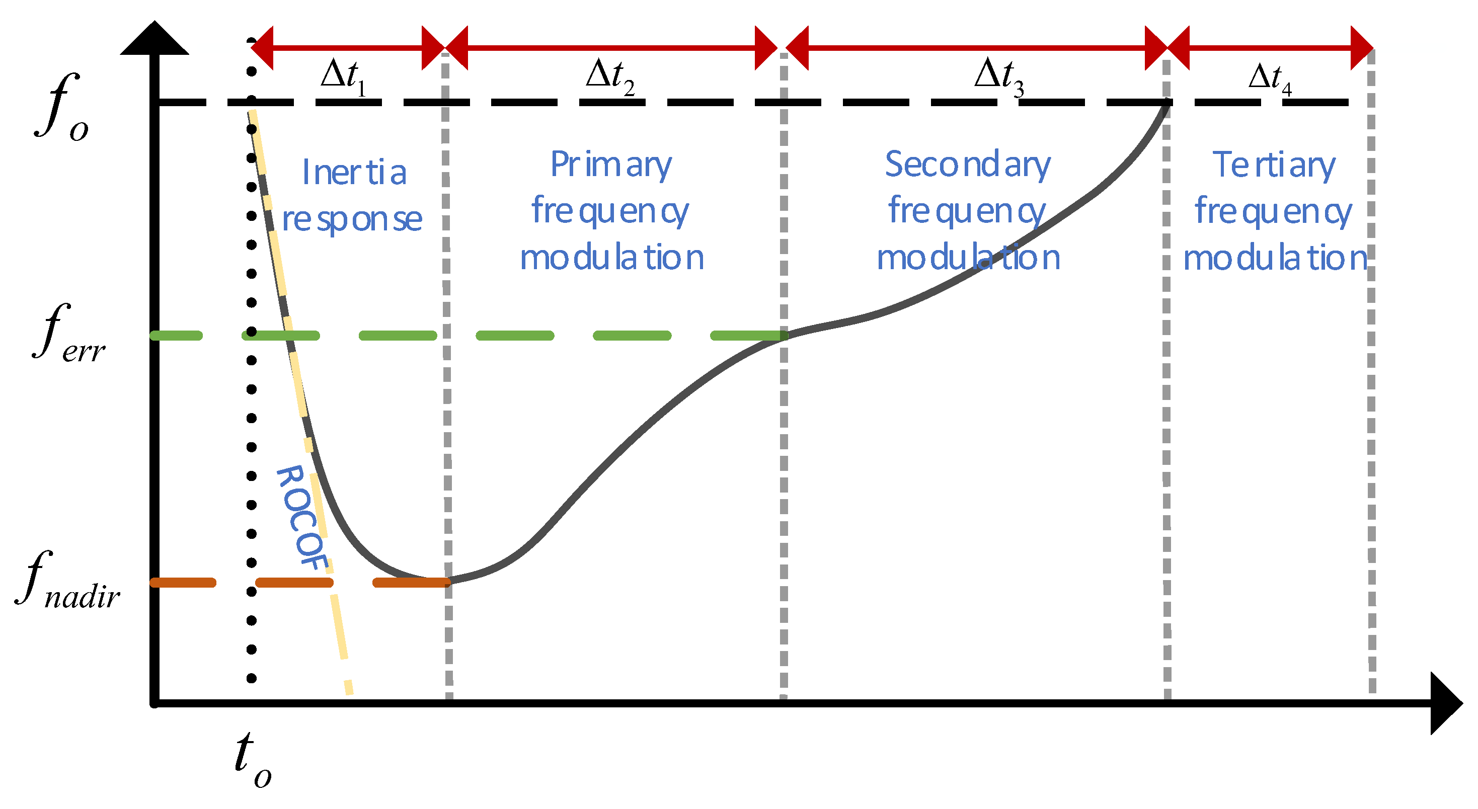
The frequency characteristic of a power system is related to the real-time active power balance of the system. Figure 1 shows the typical frequency dynamic curve of a power system after a fault disturbance, and the frequency change process can be divided into inertial response, primary frequency control, secondary frequency control, and tertiary frequency control. Some literature divides the time period before the inertial response into the fast response period.

The frequency stability of a power system may be challenged by major disturbances such as generator tripping, sudden heavy load changes, or system islanding events caused by breaker trips on interconnecting lines. After such disturbances, the system frequency will drop to a minimum point and then enter a new equilibrium point ($f_{nep}$) below the nominal value (i.e., 50 Hz). Several indicators are used to describe the dynamic performance of the system during this process, including the minimum frequency point ($f_{nadir}$), the time to reach the minimum frequency point ($t_{nadir}$), and the rate of frequency change ($Rocof$).

Inertial response takes effect immediately after a power system fault occurs before the governor begins to act. As shown by the yellow dashed line in Figure 1, the initial drop rate of the system frequency is directly proportional to the system inertia level, and the frequency drops in an approximately radial direction. In low-inertia systems, especially in power systems with a high proportion of renewable energy sources after grid connection, insufficient inertia level may lead to a rapid drop in frequency.

When the time exceeds the dead band of the speed controller, the speed controller begins to act, and the frequency drop rate gradually slows down. The speed controller increases the mechanical power output of the unit, thereby reducing the power deviation and suppressing the frequency drop. When the mechanical power is momentarily equal to the electromagnetic power, the lowest frequency drop $f_{nadir}$ appears at time $t_{nadir}$. The primary frequency control is proportional control, and the frequency rise stops at the steady-state value $f_{err}$. The duration of this stage $t_2$ is approximately 5 to 25 s.

The second frequency control stage initiates the AGC control to change the output power of the primary motor and slowly eliminate the frequency control deviation in the slow control region. The goal is to restore power balance at the rated frequency, and the duration is about 30 s to 15 min ($t_3$). Afterward, the third frequency control stage involves the unit’s rescheduling to respond to the next frequency safety incident, with a duration of more than 30 min ($t_4$).

It should be noted that, if we normalize both sides of the equation using the value of total load demand, then the damping of the load, represented by D, will be a constant that is independent of the load level. Meanwhile, the parameter H will be determined solely by the characteristics of the thermal generator and will not be affected by its installed capacity. In this article, it is assumed that all frequency equations are normalized by load demand.

2.2. Frequency Support Provided by Wind Turbines

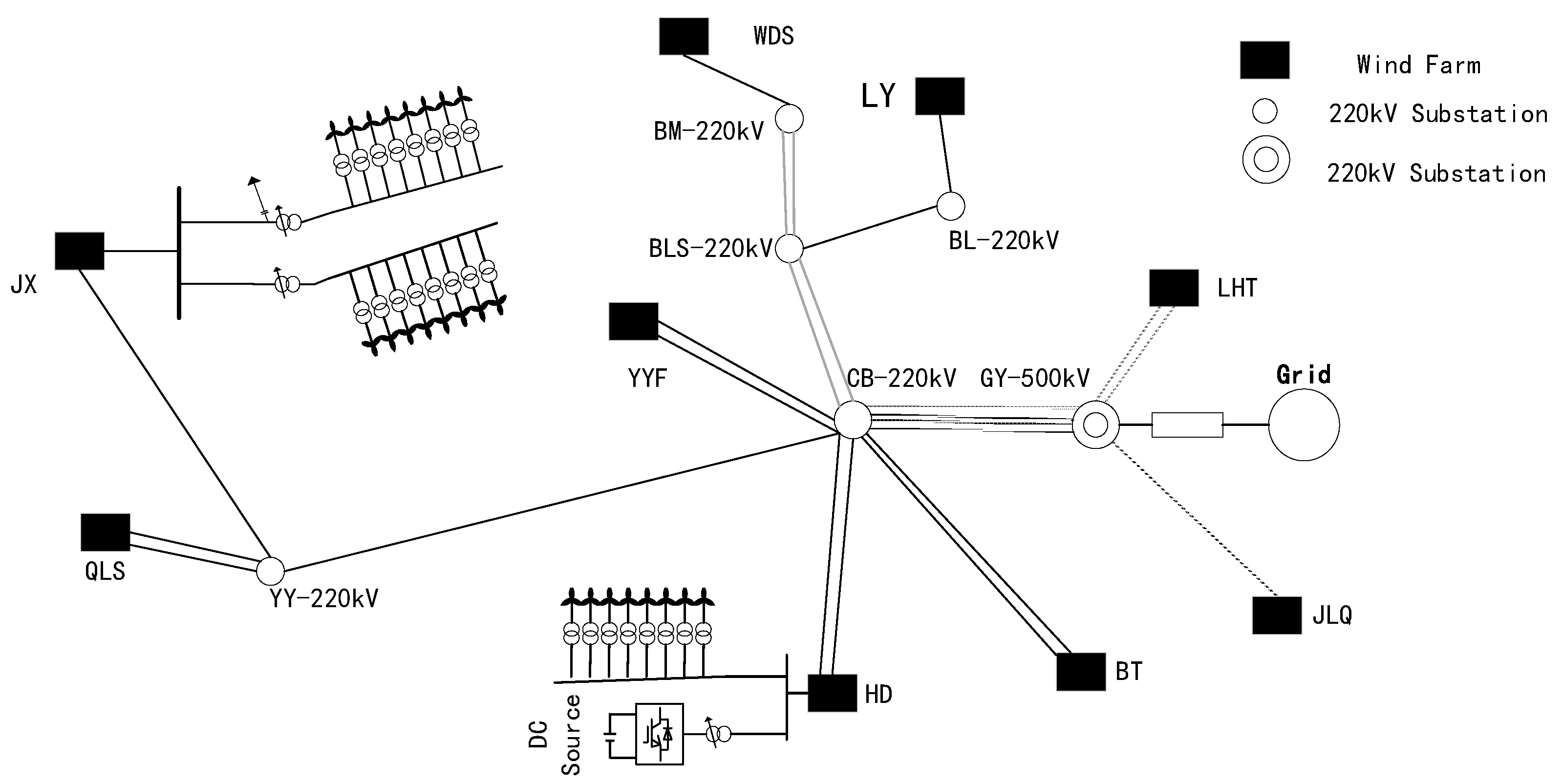
Renewable energy is connected to the grid through converters, and its power is decoupled from the grid frequency; therefore, it does not have the inertia and damping characteristics of synchronous generators. With the development of grid-connected inverters and virtual inertia control technology, renewable energy can provide frequency support through control strategies. At this point, the power system with renewable energy includes both Variable Renewable Energy (VRE) and thermal power units to provide equivalent inertia. Figure 2 presents the power system in northern China, which consists mainly of a combination of thermal generators and wind farms based on grid-connected power electronics. and the frequency response model is changed to:

$$2\left(H+{\displaystyle \sum _j{H}_{Vj}}\right)\frac{d\Delta f(t)}{dt}+D\Delta f(t)=\Delta P_m(t)+{\displaystyle \sum _j\Delta }{P}_{aj}(t)-\Delta P$$

(4)

$H_{Vj}$ represents the virtual inertia of the renewable energy system, and $\Delta P_a(t)$ represents the adjustment amount of the active power output of the VRE.

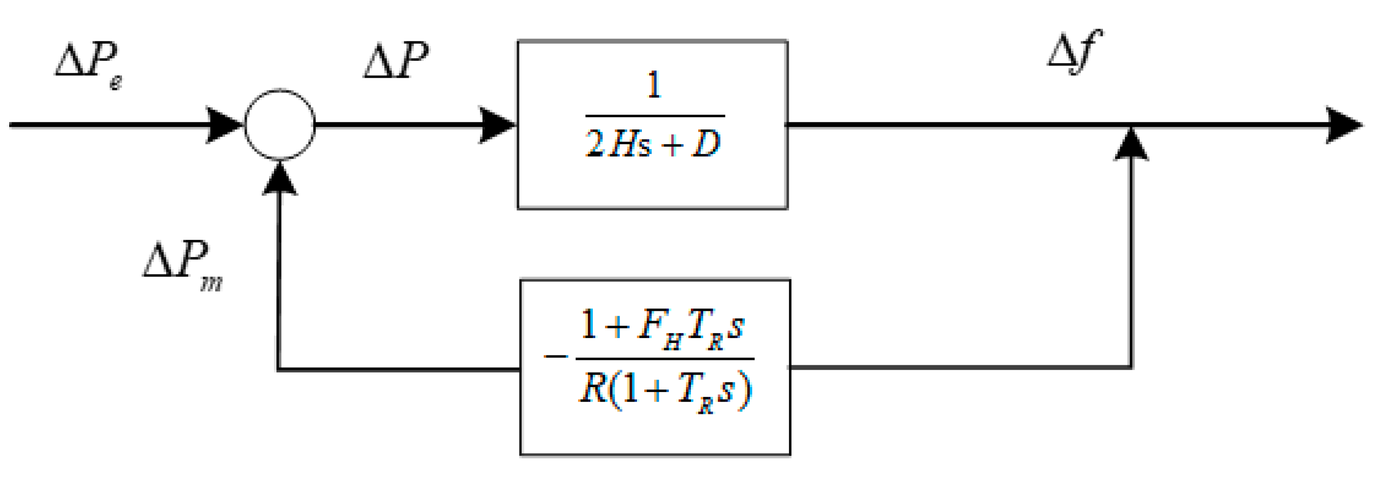
The frequency response characteristics of the system usually need to consider the regulating effect of damping, and the change of mechanical power is the co-determination determined by the governor and turbine characteristics. Figure 3 presents the frequency response model of the aggregated system, whereby the time domain expression of the system after power disturbance $\Delta P$ can be calculated:

$$\Delta f=\frac{R\Delta P}{DR+1}\left[1+\alpha e^{-\zeta {\omega }_{n}t}\sin \left({\omega }_e+\phi \right)\right]$$

(5)

The frequency security index is represented by the following equation:

$$\{\begin{array}{l}{t}_{\mathrm{nadir} }=\frac{1}{{\omega }_d}\arctan \left(\frac{{\omega }_d{T}_R}{\zeta {\omega }_d{T}_R-1}\right)\hfill \\ \Delta f_{\mathrm{nadir} }=\frac{R\Delta P}{DR+1}\left(1+\sqrt{1-{\zeta }^2}\alpha e^{-\zeta {\omega }_n{t}_{nadir}}\right)\hfill \\ \begin{array}{l}{f}_{\mathrm{nadir} }=f_0-\Delta f_{\mathrm{nadir} }\\ Rocof=\frac{d\Delta f(t)}{dt}=\frac{\Delta P_m(\mathrm{t})-\Delta P_e(t)}{2H}\end{array}\hfill \end{array}$$

(6)

where

$$\{\begin{array}{l}a=\sqrt{\frac{1-2T_R\zeta {\omega }_n+T_R^2{\omega }_n^2}{1-{\zeta }^2}}\hfill \\ {\omega }_d={\omega }_n\sqrt{1-{\zeta }^2}\hfill \end{array}$$

(7)

and

$$\varphi ={\varphi }_1-{\varphi }_2={\tan }^{-1}\left(\frac{{\omega }_d{T}_R}{1-\varsigma {\omega }_n{T}_R}\right)-{\tan }^{-1}\left(\frac{\sqrt{1-{\varsigma }^2}}{-\varsigma }\right)$$

(8)

$$K_m=\frac{P_m \mathrm{in} \mathrm{MW} }{S_{SB}}=\frac{1}{S_{SB}}{\displaystyle \sum _i{S}_{Bi}}{F}_{Pi}\left(1-f_{SR}\right)=F_P\left(1-f_{SR}\right)$$

(9)

Equation (6) represent the time-domain expression of the lowest point of the system frequency, the rate of frequency change, and the time of the lowest point of frequency drop, which are key indicators representing the frequency change after system disturbance. More details can be found in [25].

2.3. Modeling and Linearization of Safety Constraints for High Ratio Wind Power Frequency

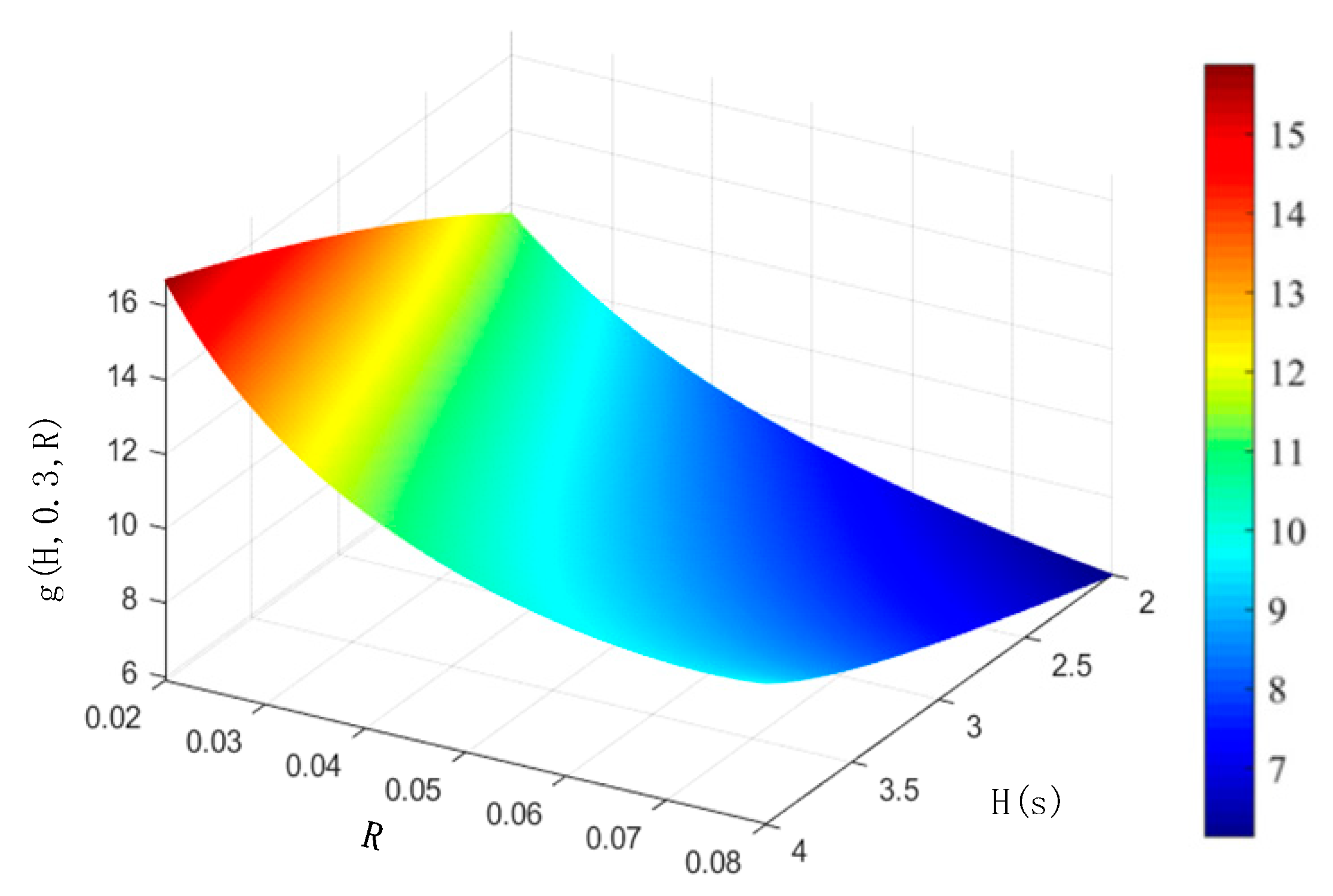
In this section, due to the complexity of the high-order non-linear function $g(H,F_H,R)$ mapping between the minimum frequency point and the shortage power, when $F_H$ is fixed, the $g$ function has a monotonic characteristic in a local range of a single parameter, as shown in Figure 4. However, it is still difficult to handle for establishing a constraint model. Therefore, it is necessary to segment and linearize the function, so that it can be included in the unit dispatch model as a solvable linear programming problem.

This subsection uses the piecewise linearization method to linearize the frequency power mapping function. First, a series of sample points ${\mathrm{g}}_k=g\left(H_k,F_{Hk},R_k\right)$ are generated through equation $\mathrm{g}\left(H,F_H,R\right)$, and the generated sample points are divided into K sample subspaces. In order to enable the resulting approximate function to be linearly represented by decision variables, [$H_k$$\frac{F_{Hk}}{R_k}$$\frac{1}{R_k}$] is selected as the variable for the sub-sample space. By establishing the following optimization model, the cutting plane parameters corresponding to each subspace can be calculated.

$$\min {\displaystyle \sum _{k\in S_j}Er{r}_k}$$

(10)

$$\begin{array}{l}s.t.\forall k\in S_j\\ \{\begin{array}{l}Er{r}_k=g(H_k,F_{Hk},R_k)-({\beta }_j^c+{\beta }_j^H{H}_k+{\beta }_j^F\frac{F_{Hk}}{R_k}+{\beta }_j^R\frac{1}{R_k})\\ Er{r}_K>=0\end{array}\end{array}$$

(11)

Since the optimization model specifies that the error between the original function plane and the hyperplane is positive, the resulting linearized function $\mathrm{g}\left(H,F_H,R\right)$ is more conservative than the original high-order function, strictly satisfying the frequency safety constraint. The linearization error can be controlled by the number of subspaces. In this paper, $N_J$ is set as 100 and the relative error is less than 3%.

Therefore, the frequency safety margin can be determined by the minimum value of the product of frequency deviation and all approximate hyperplanes, as shown in the following equation:

$$\Delta {\overline{P}}_j=\left(f_0-\underset{}{{\underset{\_}{f}}_{\min }}\right)\cdot \left({\beta }_j^c+{\beta }_j^H{H}_k+{\beta }_j^F\frac{F_{Hk}}{R_k}+{\beta }_j^R\frac{1}{R_k}\right)$$

(12)

3. Considerations about the Frequency Safety Unit Commitment and Dispatch Model with Wind Power Forecasting Errors

Due to the existence of forecasting errors, high-proportion offshore wind power cannot provide the expected synthetic inertia, resulting in difficulty in maintaining the system inertia with a high proportion of synthetic inertia to meet the requirements of unit frequency safety. Therefore, it is necessary to consider the impact of wind power forecasting errors on system frequency safety and total operating costs in the dispatch model with a high proportion of offshore wind power. This article establishes a two-stage day-ahead dispatch model. The first stage determines the start–stop plan for the units, and the second stage considers the impact of wind power forecasting errors on frequency safety under the unit combination determined in the first stage, in order to seek a unit dispatch plan that minimizes the total system cost while tolerating the forecasting errors.

3.1. Unit Commitment Model Considering Frequency Safety Constraints

The objective function is to minimize the operating cost over time periods from 1 to $N_T$, including start-up cost, shutdown cost, total output cost, and load shedding cost. The objective function is shown as follows:

$$\begin{array}{l}\min C^{sys}={\displaystyle \sum _{t=1}^{N_T}{\displaystyle \sum _{g=1}^{N_G}(C_g^{G,SU}{x}_{g,t}^{G,SU}+C_g^{G,SD}{x}_{g,t}^{G,SD}+C_g^G{P}_{g,t}^G}}+C_g^{G,B}{x}_{g,t}^G)\\ +{\displaystyle \sum _{t=1}^{N_T}{\displaystyle \sum _{n=1}^{N_N}\mathrm{VoLL}}}\cdot D_{n,t}^{Cur}\end{array}$$

(13)

The Renewable Energy Operational Constraints are as follows:

$$0\le P_{w,t}^W\le P_{w,t}^{W, \mathrm{Fore} },\forall w,\forall t$$

(14)

$$0\le P_{pv,t}^{pv}\le P_{pv,t}^{pv, \mathrm{Fore} },\forall pv,\forall t$$

(15)

Constraints (14) and (15) means that the actual wind power and photovoltaic output cannot be greater than the predicted value.

The conventional unit operating constraints are as follows:

$$x_{g,t}^G{P}_g^{G,Min}\le P_{g,t}^G\le x_{g,t}^G{P}_g^{G,Max},\forall g,\forall t$$

(16)

$$x_{g,t}^{G,SU}-x_{g,t}^{G,SD}=x_{g,t}^G-x_{g,t-1}^G,\forall g,\forall t$$

(17)

$$x_{g,t}^G,x_{g,t}^{G,SU},x_{g,t}^{G,SD}\in \{0,1\},\forall g,\forall t$$

(18)

$$P_{g,t}^G-P_{g,t-1}^G\le x_{g,t-1}^G{\alpha }_{g,t}^{G,UP}+x_{g,t}^{G,SU}{P}_g^{G,Min},\forall g,\forall t$$

(19)

$$P_{g,t-1}^G-P_{g,t}^G\le x_{g,t-1}^G{\alpha }_{g,t}^{G,DN}+x_{g,t}^{G,SD}{P}_g^{G,Min},\forall g,\forall t$$

(20)

$${\displaystyle \sum _{\tau =t-T_g^{G,on}-1}^{t-1}{x}_{g,\tau }^G}\ge x_{g,t}^{G,SD}{T}_g^{G,on},\forall g,\forall t$$

(21)

$${\displaystyle \sum _{\tau =t-T_g^{G,off}-1}^{t-1}\left(1-x_{g,\tau }^G\right)}\ge x_{g,t}^{G,SU}{T}_g^{G,off},\forall g,\forall t$$

(22)

Constraint (16) restricts the output of thermal power units to be less than the maximum capacity. Constraint (17) represents the state constraint of unit switching on and off, and the state variable is a binary variable. Equations (19) and (20) limit the unit’s ability to climb up and down per unit time. Equations (21) and (22) represents the maximum and minimum switching on and off time of the unit, limiting the frequent start and stop of the unit.

Nodal power balance constraint:

$${\displaystyle \sum _{g\in {\mathsf{\Omega }}_n^G}{P}_{g,t}^G}+{\displaystyle \sum _{w\in {\mathsf{\Omega }}_n^W}{P}_{w,t}^W}{\displaystyle \sum _{pv\in {\mathsf{\Omega }}_n^{PV}}{P}_{pv,t}^{PV}}-{\displaystyle \sum _{l\in {\mathsf{\Omega }}_n^{LS}}{F}_{l,t}^L}+{\displaystyle \sum _{l\in {\mathsf{\Omega }}_n^{LE}}{F}_{l,t}^L}=D_{n,t}^{Fore}-D_{n,t}^{Cur},\forall n,\forall t$$

(23)

$$0\le D_{n,t}^{Cur}\le D_{n,t}^{Fore},\forall n,\forall t$$

(24)

Equation (23) ensures the power balance between the generation side and the load side of the system at each time period, and Equation (24) limits the amount of load abandonment to be less than the predicted load value.

The transmission line power constraints are as follows:

$$F_{l,t}^L=B_l^L\left({\theta }_{l(+),t}-{\theta }_{l(-),t}\right),\forall l,\forall t$$

(25)

$$-\pi \le {\theta }_{n,t}\le \pi ,\forall l,\forall t$$

(26)

$$-F_l^{L,Max}\le F_{l,t}^L\le F_l^{L,Max},\forall l,\forall t$$

(27)

Constraint (25) represents the DC power flow equation and Equations (26) and (27) represent the node phase angle constraint and the maximum capacity constraint of the transmission line.

The system reserve power constraint is as follows:

$$\begin{array}{l}{\displaystyle \sum _g{x}_{g,t}^G}{P}_g^{G,Max}+{\displaystyle \sum _w{P}_{w,t}^{W, \mathrm{Fore} }}+{\displaystyle \sum _b{P}_b^{B,Max}}+{\displaystyle \sum _n{D}_{n,t}^{Cur}}\\ \ge \left(1+r_{res}\right)\left({\displaystyle \sum _n{D}_{n,t}^{\mathrm{Fore} }}+{\displaystyle \sum _w{P}_{w,t}^{W, \mathrm{Fore} }}+{\displaystyle \sum _{pv}{P}_{pv,t}^{PV, \mathrm{Fore} }}\right),\forall t\end{array}$$

(28)

Equation (28) indicates that the power output on the power generation side of the system needs to be greater than the power consumption on the load side to provide backup power for secondary frequency regulation of the system. Typically, a reserved proportional backup capacity is used for scheduling. In this article, a 10% reserve of the power consumption capacity is set as the reserve power.

The frequency safety constraints are as follows:

$$H_t=\frac{1}{{\displaystyle \sum _n{D}_{n,t}^{Fore}}}\left({\displaystyle \sum _g{x}_{g,t}^G}{H}_g^G{P}_g^{G,Max}+{\displaystyle \sum _w{u}_{w,t}^W}{H}_w^W{P}_{w,t}^{W,Fore}\right),\forall t$$

(29)

$$F_t=\frac{1}{{\displaystyle \sum _n{D}_{n,t}^{Fore}}}\left({\displaystyle \sum _g{u}_{g,t}^G}\frac{K_{mg}{F}_g^G}{R_g^G}{P}_g^{G,Max}\right),\forall t$$

(30)

$$\frac{1}{R_t}=\frac{1}{{\displaystyle \sum _n{D}_{n,t}^{Fore}}}\left(\begin{array}{l}{\displaystyle \sum _g{u}_{g,t}^G}\frac{K_{mg}}{R_g^G}{P}_g^{G,Max}+{\displaystyle \sum _w{u}_{w,t}^W}\frac{1}{R_w^W}{P}_{w,t}^{W,Fore}\hfill \\ +{\displaystyle \sum _{pv}{u}_{pv,t}^{PV}}\frac{1}{R_{pv}^{PV}}{P}_{pv,t}^{PV,Fore}\hfill \end{array}\right),\forall t$$

(31)

$$0\le u_{g,t}^G\le x_{g,t}^G,u_{g,t}^G\in \{0,1\},\forall g,\forall t$$

(32)

$$\left(f_0-{\underset{\_}{f}}_{\min }\right)\cdot \left({\beta }_j^c+{\beta }_j^H{H}_k+{\beta }_j^F\frac{F_{Hk}}{R_k}+{\beta }_j^R\right)\ge \Delta P,\forall j$$

(33)

$$\frac{d\Delta f(t)}{dt}=\frac{\Delta P}{2H}\le Roco{f}_{\max }$$

(34)

Equations (29)–(31) represent the frequency response model parameters of a high proportion wind power aggregation system. Since the frequency regulation capacity of each unit is related to its own capacity, assuming that the total generating capacity of the system is equal to the predicted value of the total load, the system aggregate parameters are determined by the frequency regulation status of each unit and the maximum output power Co-determination. Equation (32) indicates that the frequency regulation status variable composed of binary numbers is limited by the operating status of the unit, and Equation (33) limits that the lowest frequency point in the process of system frequency disturbance is not less than the specification value. Equation (34) limits the initial frequency drop speed.

Based on the objective function (13) and constraints (14)–(34), the proposed frequency safety model can be constructed, which can be solved through existing solvers.

3.2. Set of Uncertainties in Offshore Wind Power Forecasting Errors

In traditional unit commitment, as new energy sources account for a small proportion, a large number of online thermal power units participate in frequency response, and the overall system inertia is sufficient, so the prediction error of new energy only affects the power balance, with little impact on the system frequency response. However, as the scale of offshore wind power increases, its impact on the power system gradually increases, and the influence of wind power prediction errors on system frequency needs to be considered. Wind power units are controlled and connected to the grid by power electronic devices to provide virtual inertia, and wind power forecasts determine the estimated size of the synthetic inertia that can be provided. When the forecast produces errors, it will affect the frequency response of the power system, which is mainly composed of generated synthetic inertia.

The uncertainty of wind power output in the unit combination model can be represented by an error set to indicate the fluctuation range of wind power output forecast. The conventional box-type uncertainty set takes extreme environments that occur with a very low probability as the worst-case scenario to establish unit scheduling plans, which results in excessively high total operating costs. Therefore, this paper adopts a budget-based set to represent the uncertainty interval of new energy.

$$U_1=\left\{\xi :{\displaystyle \sum \left|\frac{{\xi }_i-{\widehat{\xi }}_i}{\overline{{\xi }_i}-\underset{\_}{\xi }}\right|}\le \mathsf{\Gamma },\left|\xi \right|\le e\right\}$$

(35)

In the formula, $\overline{{\xi }_i}$ and $\underset{\_}{{\xi }_i}$ represent the upper and lower bounds of the uncertain parameter i, $\widehat{\xi }$ represents the predicted value of the uncertain parameter, and $\mathsf{\Gamma }$ represents the number of uncertain parameters that can change to the maximum deviation. The size of $\mathsf{\Gamma }$ determines the conservatism of the system. The first to propose this type of uncertainty set were Bertsimas and Sim [26]. This type of uncertainty set is constructed based on the relative deviation of uncertain parameters and can accurately reflect the fluctuation of parameters.

3.3. Two-Stage Robust Optimization Model Considering Wind Power Forecast Error

This article proposes a two-stage robust optimization model considering wind power forecast uncertainty. In the first stage, the start–stop status of traditional units and whether that participates in frequency regulation are determined. As shown in the equation above, the system’s inertia, error correction coefficient, and generator reheating time constant are determined by the online status and whether the unit participates in frequency regulation. Therefore, the scheduling model under the first stage will ensure that the system’s frequency does not exceed a predetermined value at the lowest point under a pre-set affordable power shortage. Additionally, to meet the requirement that the initial frequency drop rate does not exceed the set value, the system’s inertia will be maintained at a corresponding value or higher. In the second stage, the power balance between generation and load is considered. The second stage seeks to minimize the cost while maintaining power balance under the worst-case scenario of wind power forecast deviation when the unit start–stop status is determined in the first stage.

The operating objective of the proposed model in this paper is to minimize the daily operating cost, as shown in the equation. The objective function includes the costs of unit start-up and shut-down, the costs of power generation from each unit, and the cost of abandoned load. The constraints to be satisfied include equality constraints, inequality constraints, and so on.

Its compact form can be expressed as:

$$\min C_{1}x+C_{2}y$$

(36)

$C_1$ represents the start-up and shut-down cost of the units; $C_2$ represents the generation cost and the cost of shedding load; $x$ represents the binary decision variables that indicate the start-up and shut-down states of the units; $y$ represents the continuous variables that represent the output of each unit, the output of the new energy, and the load shedding. The proposed UC model can be expressed as a typical two-stage formulation. The first-stage problem is to determine the operating states of the units using binary decision variables $x$ before the future wind power output is realized, after the start-up and shut-down states of the units are determined. The second-stage problem is to consider the output power of each unit under the worst-case scenario when the wind power generation deviates from the predicted value. This problem can be expressed as solving the min max min objective function:

$$\underset{x}{\min } \underset{\xi }{\max } \underset{y}{\min } C_{1}x+C_{2}y(\xi )$$

(37)

$$\mathrm{s}t.\{\begin{array}{l}A\mathrm{y}+Bx\ge E\hfill \\ C\mathrm{y}+Dx=F\hfill \end{array}$$

(38)

The variables x and y in the equation are optimization variables, and their specific expressions are:

$$\{\begin{array}{l}x={[x_{g,t}^G,x_{g,t}^{G,SU},x_{g,t}^{G,SD},u_{g,t}^G,u_{w,t}^W,u_{pv,t}^{PV}]}^T\hfill \\ y={[P_{g,t}^G,P_{w,t}^W,F_{l,t}^L,{\theta }_{n,t},D_{n,t}^{Cur}]}^T\hfill \end{array}$$

(39)

A, B, C, and D are the coefficient matrices of the variables under the corresponding constraints, E. F is a constant column vector. In Equation (39), the first line of the constraint condition represents the inequality constraints containing uncertain variables in the robust optimization model, including Equations (17), (23), and (25). The second line represents all equation constraints in the model, including the remaining equations in constraints (14)–(34).

4. Solution of the Model

For the conventional solution algorithms, it is generally difficult to solve the two-stage robust optimization model mentioned above, and the modified Bender decomposition method can be used for solution [27]. However, when extending to multi-stage robust optimization problems, decision criteria need to be used for approximate solution. The decision criteria methods currently used mainly include affine, piecewise affine, and trigonometric polynomial functions. In this paper, the affine decision criterion is adopted to represent the complex mapping relationship between random variables $\xi$ and decision variables $y$ by a linear feasible domain. The original problem is approximated and transformed into an easy-to-solve problem, and then:

Replacing the second-stage variable $y$ in the two-stage problem with the following linear equation with uncertain parameters can effectively reduce the number of iterations in traditional algorithm and obtain optimal solutions in some engineering applications.

$$y=y_0+Y\xi$$

(40)

where $y_0$ is the intercept and $Y$ is the coefficient. At this point, the two-stage problem is transformed into:

$$\underset{x}{\min } \underset{\xi }{\max } \underset{y}{\min } C_{1}x+C_2(y_0+Y\xi )$$

(41)

In this problem, the second stage is to determine the output of each node unit under the worst-case scenario. For any uncertain variable in the model, there exists a corresponding scheduling value of the continuous variable $y$ and the mapping relationship between the uncertain parameters and the continuous decision variables is complex and difficult to solve in the second stage. In the solution process, a large number of nonlinear problems are often encountered. By using the affine decision rule method to establish the linear mapping relationship between the continuous decision variables and the uncertain variables, the two-stage problem can be transformed into a conventional robust problem. At this point, as shown in the equation, the result obtained by exchanging the position of $y$ and the uncertain variable $\xi$ is still the optimal scheduling solution under the affine linear decision approximation.

$$\underset{x}{\min } \underset{y}{\min } \underset{\xi }{\max } C_{1}x+C_2(y_0+Y\xi )$$

(42)

$$\underset{x}{\min } \underset{\xi }{\max } C_{1}x+C_2(y_0+Y\xi )$$

(43)

At this time, the feasible solution set of the second stage $y$ determined by $\{y:\equiv \to {ℝ}^{N_2}\}$ converts to $\left\{\exists Y\in {ℝ}^{N_2\times K}, y_0\in {ℝ}^{N_2}, \mathrm{y}(\xi )=Y\xi +y_0\right\}$, which is defined by finite parameters, and the original two-stage model is transformed into a solvable robust formal model.

$$\begin{array}{ll}& Ay(\xi )+Bx\ge E(\xi )\hfill \\ \hfill \Rightarrow & A({\mathrm{y}}_o+y\xi )+Bx\ge E_0+\overline{E}\xi \hfill \\ \hfill \Rightarrow & \underset{a}{\underbrace{A{\mathrm{y}}_o+Bx-E_0}}+\underset{b}{\underbrace{(Ay-\overline{E})}}\xi \ge 0\hfill \end{array}$$

(44)

In summary, the model is a mixed-integer programming problem and can be effectively solved using existing solvers.

5. Case Study

5.1. Basic Data

This article verifies the calculation examples using the IEEE 24-node 38-bus system. The total load is set to 2850 MW, and the frequency safety constraint is set according to the European grid specification with an initial droop rate not exceeding 0.125 Hz/s [28]. It is assumed that the lowest frequency point is not less than 49.6 Hz. The modified generation combination is shown in

Table 1. Distribution of Node Units.

Node	U155	U350	U76	U197	Wind	PV	Sum
B1			76 × 2		500		652
B3			76 × 2		500	500	1152
B6	155 × 2					500	810
B7				197 × 3			591
B15			76 × 2		500		652
B16			76 × 2			500	652
B17		350 × 2					700
B21		350					350
B22		350					350
B23	155 × 2						310
Total	620	1400	608	591	1500	1500	6319

. Information on transmission lines and load demand can be found in reference [29].

The parameters of thermal generators are listed in

Table 2. Frequency response characteristics of generators and VRE devices.

Generation Type	U76	U155	U197	U350
Capacity (MW)	76	155	197	350
Variable cost (USD/MWh)	45	30	35	20
No-load cost (USD/h)	0	0	0	0
Start-up cost (USD/MW)	6	2	4	4
Shut-down cost (USD/MW)	6	2	4	4
Minimum online time (h)	4	8	4	8
Minimum offline time (h)	4	8	4	8
Ramp capacity (s)	80%	50%	80%	50%
Minimum output	20%	35%	80%	50%

.

Table 3. Frequency response characteristics of generators and VRE devices.

Generation Type	U76	U155	U197	U350	Wind	PV
Inertia constant (s)	4	6	6	8	3	0
Turbine factor $F_H$	0.25	0.3	0.3	0.35
Governor constant	0.033	0.05	0.033	0.05
Droop of VRE					0.067	0.067

shows the frequency response characteristics of traditional generators and renewable energy devices. The frequency support capability of VRE is based on [30]. As the range of the grid-connected inverters installed in VRE is large, we conservatively assume that the frequency support capability is 50% of the conventional thermal power generation capacity.

5.2. Analysis of Results

In order to ensure that the lowest frequency point of the system does not exceed the specified value under the set power shortage threshold, the start–stop status of thermal power generation units in each period of the system is shown in Figure 5. It can be seen that, when wind power is high, the number of unit starts will also increase, but the unit output will be lower. At this time, the thermal power generation units can not only meet the low output requirements but also have frequency modulation capabilities.

Figure 6 shows the output of each unit, photovoltaic, and wind turbine during different time periods, meeting the power balance requirements of each node and ensuring the stability of the system frequency.

Table 4. Operation cost of different schemes.

	Operating Costs (USD)	Abandon Wind	Abandon PV
Wind power error is not considered	690,130	1.61%	1.42%
Considering wind power error	725,175	2.78%	3.12%

shows that the operating cost of the robust model considering frequency security constraints is higher than that of the frequency security model that does not consider wind power uncertainty. When the total cost is converted into hourly costs, it can be found that the robust model will set more conventional units to remain online when wind power output is high. This is because, when wind power output is high, the system inertia will be lower. Since most of the system inertia is composed of synthetic inertia provided by new energy sources such as wind power, the system will exhibit poorer frequency characteristics in the event of prediction errors. Therefore, more conventional units need to be set online to provide more mechanical inertia.

Figure 7 analyzes the system inertia composition when the prediction error is 0.1. From Figure 7, it can be seen that, after 9 pm every day until 5 am the next day, new energy sources such as wind and photovoltaics cannot provide virtual inertia for frequency regulation due to their low output. At this time, the system inertia is mainly provided by thermal power units. However, when the output of new energy sources is high from 6 am to 8 pm, virtual inertia can be provided to participate in frequency regulation, and the maximum inertia that can be provided is about 2 s. This ensures that the power grid can meet the system frequency safety requirements even during periods when the physical inertia of thermal power units is insufficient.

From

Table 5. Influence of the number of uncertain variables on the operation cost ($\overline{{\xi }_i}$= 0.1).

$$\mathbf{\Gamma }$$	Operating Costs (USD)	Gap with Deterministic Scheduling %
0	690,130	0
5	704,626	2.1005
10	712,465	3.2363
15	719,892	4.3125
20	731,353	5.9732
25	747,656	8.3344
30	755,635	9.4917
35	768,765	11.3942
40	784,563	13.6833

, it can be seen that, when Gamma is 0, the proposed model is equivalent to a deterministic optimization scheduling problem. As the value of Gamma increases, more parameters are allowed to reach their maximum deviation in the model, and the scheduling cost of the system increases as uncertainty increases. When the increase in operating costs is mainly due to the uncertainty in the prediction of new energy sources such as wind and photovoltaics, prediction errors directly affect the frequency support provided by new energy sources because the relevant parameters affecting frequency, such as system inertia and regulation coefficient, are directly related to the predicted values of new energy sources. At this time, more conventional units need to remain online to provide corresponding frequency support, so as Gamma increases, the frequency support provided by new energy sources becomes unreliable, and more conventional units need to be used, which leads to higher operating costs.

In

Table 6. The impact of different prediction errors on operating costs.

$\mathbf{Prediction} \mathbf{Error} \overline{\mathit{\xi }}$	Cost (USD)	Gap with Deterministic Scheduling %
0	690,130	0
0.1	725,175	5.07800
0.2	745,764	8.0614
0.3	793,468	14.9737
0.4	832,354	20.6083
0.5	874,765	26.7537
0.6	944,578	36.8696
0.7	994,575	44.1142
0.8	1,027,654	48.9073
0.9	1,082,357	56.8338
1	1,122,346	62.6282

, it can be seen that the degree of deviation of new energy source prediction errors from the actual values, relative to the reference curve, is multiplied by the prediction error $\overline{\xi }$. When $\overline{\xi }$ = 0, it is equivalent to a deterministic scheduling model considering frequency safety constraints. As the deviation value continues to increase, the wind power output becomes more unstable, and the frequency characteristic parameters such as inertia of the power system fluctuate greatly, reducing system safety. At this time, the operating cost continues to increase, and the inertia component of the system mainly consists of traditional units.

Figure 8 shows the operating cost and cost difference ratio between the deterministic dispatch plan and the dispatch plan considering wind power prediction errors under different levels of new energy capacity. As the proportion of new energy increases, the uncertainty of wind power prediction has a greater impact. Therefore, as the new energy capacity increases, the cost required for the plan considering prediction errors increases more in order to meet the frequency safety requirements of the system.

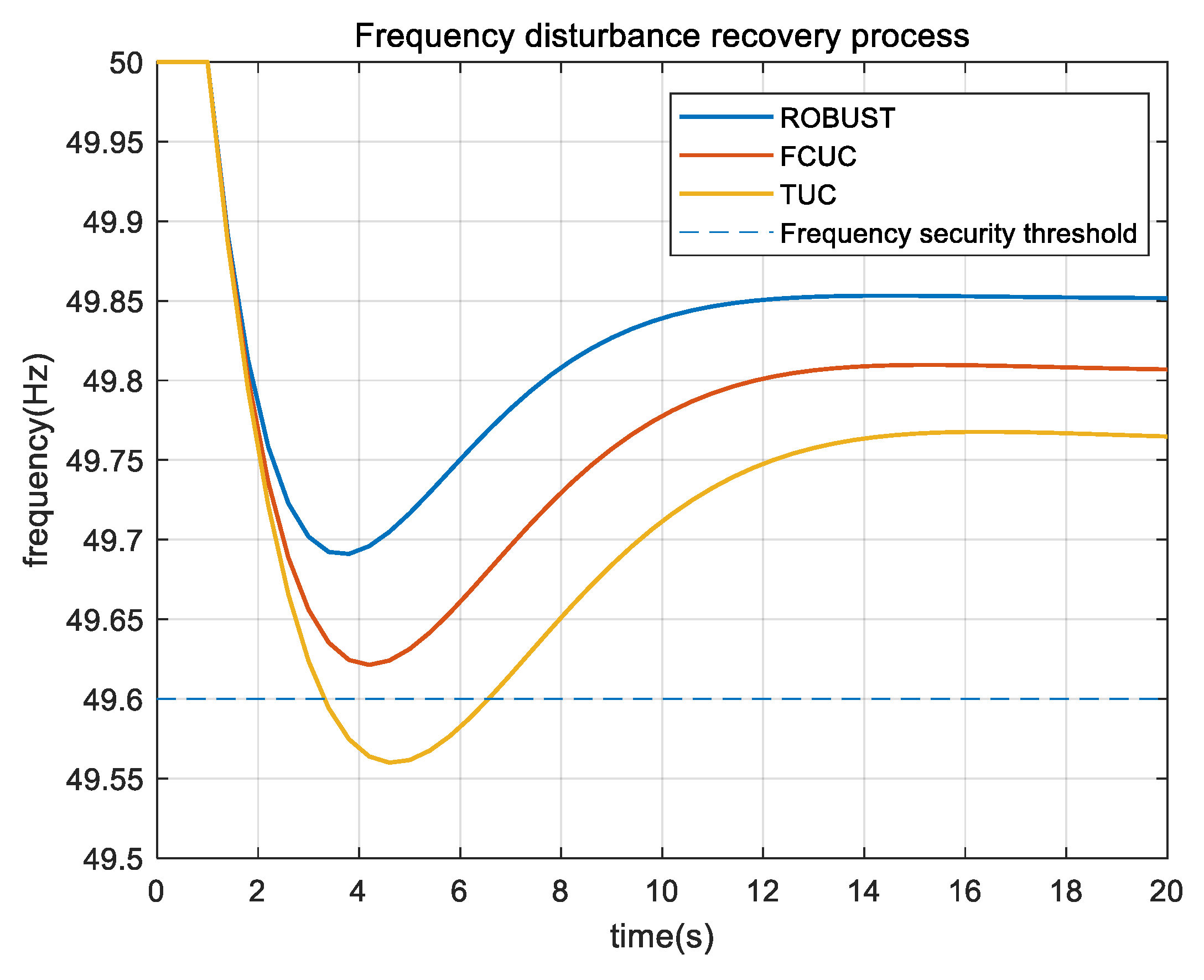
As shown in Figure 9, we compared the frequency response capability of the proposed model with Frequency Constrained Unit Commitment Model (FCUC) and Traditional Unit Commitment Model (TUC). The unit model without considering frequency safety constraints is more severe than the scheduling scheme that considers frequency safety constraints in terms of both frequency drop rate and lowest frequency point when facing the mismatch between load and generator power. When the system is in a safe margin, the proposed scheme in this paper can control the frequency safety index well without exceeding the limit. This is because the proposed scheme in this paper considers the Rocof constraint and frequency lowest point constraint in scheduling, which keeps the total system’s inertia related to frequency at a certain level to reduce the frequency drop rate. By controlling the frequency regulation capability of new energy sources, all parties involved in scheduling can coordinate to support frequency and ensure that the dynamic characteristics of the system frequency meet the frequency safety settings. When the power shortage amount exceeds the set safety margin, the proposed scheme can still perform better than the conventional unit scheduling scheme.

6. Conclusions

This article establishes a frequency safety unit optimization scheduling model that considers the uncertainty due to the grid connection of new wind power systems and the problem of inertia deficiency based on a two-stage robust optimization method. The analysis results show the following:

• The model proposed in this paper can effectively solve the frequency problem in power systems with large-scale integration of new energy sources. It quantifies the frequency safety index after the occurrence of power disturbances in the system, and through the rational scheduling of units, it ensures that there are enough frequency support units participating in the frequency regulation response in each period. The model can guarantee that the frequency drop rate and the lowest frequency point do not exceed the specified values when the system experiences a power shortage.
• This paper fully considers the impact of wind power prediction errors on the overall frequency characteristics of the system by establishing the relationship between new energy, system inertia, and regulation coefficients affecting frequency. By solving the two-stage model, the obtained unit combination scheme can ensure rapid and stable system frequency in each period within the prediction error setting range.
• The robust unit scheduling model proposed in this paper, which considers the uncertainty of wind power output, can provide a reference for the auxiliary service market of wind power units and other units in future power systems, where all participating units respond to the frequency regulation with their output below the safety margin set in the paper.

In the unit scheduling cost studied in this paper, only the start–stop status and output cost of conventional units were considered, and the control of the frequency response provided by wind power was based on whether it participated in frequency regulation. In future research, the cost analysis of wind power units providing frequency regulation services through collaborative control can be considered, and a scheduling scheme considering the temporal and spatial correlation of units can be established, fully utilizing the frequency regulation characteristics of new energy units.

References

- Ember. 2023 Global Wind Report [EB/OL]. 2023. Available online: https://gwec.net/globalwindreport2023/ (accessed on 19 June 2023).
- Kundur, P. Power System Stability and Control; McGraw-Hill: New York, NY, USA, 1994. [Google Scholar]
- Hou, Q.; Du, E.; Zhang, N.; Kang, C. Impact of High Renewable Penetration on the Power System Operation Mode: A Data-Driven Approach. IEEE Trans. Power Syst. 2020, 35, 731–741. [Google Scholar] [CrossRef]
- Fernández-Guillamón, A.; Gómez-Lázaro, E.; Muljadi, E.; Molina-García, A. Power systems with high renewable energy sources: A review of inertia and frequency control strategies over time. Renew. Sustain. Energy Rev. 2019, 115, 109369. [Google Scholar] [CrossRef] [Green Version]
- Zhang, C.; Liu, L.; Cheng, H.; Lu, J.; Zhang, J. Review and Prospects of Planning and Operation Optimization for Electrical Power Systems Considering Frequency Security. Power Syst. Technol. 2022, 46, 250–264. [Google Scholar]
- Restrep, J.F.; Galiana, F.D. Unit commitment with primary frequency regulation constraints. IEEE Trans. Power Syst. 2005, 20, 1836–1842. [Google Scholar] [CrossRef]
- Gu, H.; Yan, R.; Saha, T.K. Minimum Synchronous Inertia Requirement of Renewable Power Systems. IEEE Trans. Power Syst. 2018, 33, 1533–1543. [Google Scholar] [CrossRef] [Green Version]
- Wang, T.; Miao, S.; Yao, F.; Liu, Z.; Zhang, S. Day-ahead and Intra-day Joint Dispatch Strategy of High Proportion Wind Power System Considering Dynamic Frequency Response Constraints. Proc. CSEE 2023, 45, 1–19. [Google Scholar]
- Trovato, V.; Bialecki, A.; Dallagi, A. Unit Commitment With Inertia-Dependent and Multispeed Allocation of Frequency Response Services. IEEE Trans. Power Syst. 2019, 34, 1537–1548. [Google Scholar] [CrossRef]
- Yang, D.; Wang, X.; Yan, G.-G.; Jin, E.; Huang, J. Decoupling active power control scheme of doubly-fed induction generator for providing virtual inertial response. Int. J. Electr. Power Energy Syst. 2023, 149, 109051. [Google Scholar] [CrossRef]
- Yan, X.; Zhang, W.; Cui, S.; Huang, H.; Li, T. Frequency Response Characteristics and Adaptive Parameter Tuning of Voltage-Sourced Converters under VSG Control. Trans. China Electrotech. Soc. 2021, 36, 241–254. [Google Scholar]
- Nie, Y.; Liu, J.; Sun, B.; Zhao, Y.; Wu, Y. Research on Nonlinear Frequency Control Strategy of Wind Power Grid Connected System Based on Rotor Kinetic Energy Release. Proc. CSEE 2022, 10, 1–11. [Google Scholar]
- Koutroulis, E.; Kalaitzakis, K. Design of a maximum power tracking system for wind-energy-conversion applications. IEEE Trans. Ind. Electron. 2006, 53, 486–494. [Google Scholar] [CrossRef]
- Chen, J.; Liu, M.; Milano, F.; O’Donell, T. Adaptive Virtual Synchronous Generator Considering Converter and Storage Capacity Limits. CSEE J. Power Energy Syst. 2022, 8, 580–590. [Google Scholar]
- Ge, X.; Liu, Y.; Fu, Y. Distributed Robust Unit Commitment Considering the Whole Process of Inertia Support and Frequency Regulations. Proc. CSEE 2021, 41, 4043–4058. [Google Scholar]
- Zhao, C.; Wang, J.; Watson, J.P.; Guan, Y. Multi-Stage Robust Unit Commitment Considering Wind and Demand Response Uncertainties. IEEE Trans. Power Syst. 2013, 28, 2708–2717. [Google Scholar] [CrossRef]
- Xiong, P.; Jirutitijaroen, P.; Singh, C. A Distributionally Robust Optimization Model for Unit Commitment Considering Uncertain Wind Power Generation. IEEE Trans. Power Syst. 2017, 32, 39–49. [Google Scholar] [CrossRef]
- Wang, B.; Yang, D.; Cai, G. Dynamic Frequency Constraint Unit Commitment in Large-scale WindPower Grid Connection. Power Syst. Technol. 2020, 44, 2513–2519. [Google Scholar]
- Zhang, Z.; Du, E.; Teng, F.; Zhang, N.; Kang, C. Modeling Frequency Dynamics in Unit Commitment With a High Share of Renewable Energy. IEEE Trans. Power Syst. 2020, 35, 4383–4395. [Google Scholar] [CrossRef]
- Li, H.; Qiao, Y.; Lu, Z.; Baosen, Z.; Fei, T. Frequency-Constrained Stochastic Planning Towards a High Renewable Target Considering Frequency Response Support From Wind Power. IEEE Trans. Power Syst. 2021, 36, 4632–4644. [Google Scholar] [CrossRef]
- Sturt, A.; Strbac, G. Efficient Stochastic Scheduling for Simulation of Wind-Integrated Power Systems. IEEE Trans. Power Syst. 2012, 27, 323–334. [Google Scholar] [CrossRef]
- Liu, Y.; Guo, L.; Wang, C. Economic Dispatch of Microgrid Based on Two Stage Robust Optimization. Proc. CSEE 2018, 38, 4013–4022. [Google Scholar]
- Paturet, M.; Markovic, U.; Delikaraoglou, S.; Evangelos, V.; Petros, A.; Gabriela, H. Stochastic Unit Commitment in Low-Inertia Grids. IEEE Trans. Power Syst. 2020, 35, 3448–3458. [Google Scholar] [CrossRef] [Green Version]
- Ding, T.; Bo, R.; Sun, H.; Xing, F.L. A Robust Two-Level Coordinated Static Voltage Security Region for Centrally Integrated Wind Farms. IEEE Trans. Smart Grid 2016, 7, 460–470. [Google Scholar] [CrossRef]
- Shi, Q.; Li, F.; Cui, H. Analytical Method to Aggregate Multi-Machine SFR Model With Applications in Power System Dynamic Studies. IEEE Trans. Power Syst. 2018, 33, 6355–6367. [Google Scholar] [CrossRef]
- Bertsimas, D.; Sim, M. Robust discrete optimization and network flows. Math. Program. 2003, 98, 49–71. [Google Scholar] [CrossRef]
- Ayoub, J.; Poss, M. Decomposition for adjustable robust linear optimization subject to uncertainty polytope. Comput. Manag. Sci. 2016, 13, 219–239. [Google Scholar] [CrossRef] [Green Version]
- Ding, T.; Zeng, Z.; Qu, M.; Catalão, S.P.J.; Shahidehpour, M. Two-Stage Chance-Constrained Stochastic Thermal Unit Commitment for Optimal Provision of Virtual Inertia in Wind-Storage Systems. IEEE Trans. Power Syst. 2021, 36, 3520–3530. [Google Scholar] [CrossRef]
- Subcommittee, P. IEEE Reliability Test System. IEEE Trans. Power Appar. Syst. 1979, 6, 2047–2054. [Google Scholar] [CrossRef]
- Margaris, I.D.; Papathanassiou, S.A.; Hatziargyriou, N.D.; Hansen, D.A.; Sorensen, P. Frequency Control in Autonomous Power Systems With High Wind Power Penetration. IEEE Trans. Sustain. Energy 2012, 3, 189–199. [Google Scholar] [CrossRef]
Figure 1.
Power system frequency response model.
Figure 2.
China northern power grid with wind farms [24].
Figure 3.
Aggregated system frequency model.
Figure 4.
Mapping function g between the lowest point of system frequency and frequency parameters, fixed = 0.3.
Figure 5.
Unit online and offline status.
Figure 6.
Power generation results of the two-stage frequency safety constraint model.
Figure 7.
System inertia composition under = 30 = 0.1.
Figure 8.
Operation cost of each scheme under different new energy grid connection capacity.
Figure 9.
Frequency dynamic response curve under different schemes.