
Predicting Station-Level Peak Hour Ridership of Metro Considering the Peak Deviation Coefficient
1
School of Traffic and Transportation, Lanzhou Jiaotong University, Lanzhou 730070, China
2
Key Laboratory of Railway Industry on Plateau Railway Transportation Intelligent Management and Control, Lanzhou 730070, China
*
Author to whom correspondence should be addressed.
Sustainability 2024, 16(3), 1225; https://0-doi-org.brum.beds.ac.uk/10.3390/su16031225
Submission received: 25 December 2023
/
Revised: 21 January 2024
/
Accepted: 27 January 2024
/
Published: 1 February 2024
(This article belongs to the Collection Sustainable Rail and Metro Systems)
Abstract
:Subway station-level peak hour ridership (SPR) is a crucial input parameter for multiple applications, including the planning, design, construction, and operation of stations. However, traditional SPR estimation techniques may produce biased results. A unified peak hour factor (PHF) extracted from the line level is generally set for all attributed stations, which ignores the possible peak deviation that arises between the station and line and the wide variation of PHFs in practice. This study presents a comprehensive and refined estimation framework for SPR that accommodates the peak deviation context by introducing the peak deviation coefficient (PDC). Moreover, the estimation of the PDC and PHF variability is improved by constructing spatial regression based relationship models. The empirical results show that the proposed approach exhibits wider applicability and a higher prediction precision across all types of peak periods considered as compared to conventional methods (i.e., MAPE decreases of 0.115–0.351). The findings demonstrate the importance of the consideration of the peak deviation scenario and the spatial dependency in SPR estimation to achieve better decision making. Moreover, the underlying influencing mechanism of the PHF and PDC at distinct peak periods is further revealed using the spatial model. This provides critical theoretical references and policy implications to prudently deploy land-use resources to balance the travel demand between peak and off-peak periods and thus enhance the line operation efficiency.
1. Introduction
In recent years, the urban rail transit system has been aggressively constructed because of its large volume and environmental protection [1]. By the end of 2022, 545 cities had a rail transit system in operation, with 41,386.12 km worldwide. In transportation spatial networks, traffic demand and design basis are typically observed by predicting origin–destination (OD) patterns or analyzing the characteristics of hot spots [2,3]. Due to the ridership varying by the time [4], the ridership during peak hours is usually taken as the design basis of the urban rail transit system. Thus, accurate station-level peak hour ridership (SPR) estimation is the basis for station planning, facility design, and operational decisions [5]. Currently, traditional methods generally estimate the SPR based on a unified peak hour factor (PHF) that is extracted from the line level, which relies on the assumption that the station-level ridership peak hours and PHF are roughly equal to those at the line level [6,7]. Although this greatly simplifies the estimation process, erroneous estimation results may be produced due to its assumption that the station peak and the metro line peak simultaneously occurred.
However, the peak hour of stations may not completely align with that of the attributed line [8]. This phenomenon has been increasingly revealed in numerous cities worldwide in recent years, such as Osaka, Japan (an approximate half-hour peak deviation for most stations); Shanghai, China (30.36% of stations) [9]; and Chongqing, China (69.44%–70.83% of stations) [10]. In addition to the aforementioned cities, it has also been observed in regions such as London in the UK, Los Angeles in the US, Ontario Province in Canada, and Seoul in South Korea that the time distribution of ridership in stations has different forms [11,12,13,14]. The ignorance of peak deviation may induce underestimated SPR values, which can result in an insufficient capacity design at station service facilities and consequently lead to traffic congestion. A new specification, namely the Code for Prediction of Urban Rail Transit Ridership in China, supplements the requirement for estimating station ridership within station peak hours. This specification is aimed at stations whose peak time does not completely coincide with that of the line.
To calibrate the SPR, Chen et al. developed an index called the peak deviation coefficient (PDC) to measure the magnitude of the station ridership deviation between two peaks [8]. Subsequently, several methods have been proposed to determine the PDC and can be generally divided into three categories: statistical techniques, local models, and global models. For instance, Yu et al. utilized a statistical analysis technique to explore the associations between the PDC and the land-use type of the land surrounding the station [10] and applied a local model, namely a geographically weighted regression (GWR), to investigate the determinants of the PDC [15]. However, the application of these methods is limited to the ridership analysis of existing stations rather than the ridership estimation of planned stations due to the lack of a quantitative relationship model or the local suitability of the model parameters. Aiming at a PDC estimation, local models [16] have been employed to construct PDC relationship models. Nevertheless, these methods tend to assume that the PDC estimation is independent across stations. They ignore the fact that the subway system is a network in which the stations exhibit strong spatial correlations, which means that the ridership characteristic of a station might also be influenced by the attributes of its neighbors. The omission of the spatial dependency of station ridership in these models might produce erroneous estimations and interpretations for a PDC estimation.
Moreover, in practice, station PHF values vary widely with their station attribute characteristics and geographical location rather than having a unified value. Two types of station PHFs may be distinguished in existing research depending on whether the consistent peak assumption is adopted. Under the assumption of a consistent peak, Liu et al. found that the PHF value of subway stations in Guangzhou, China, changed in a wide range of 0.036 to 0.322 [17]. Considering the peak deviation phenomena, Zhao et al. revealed that the actual PHF values of stations in Nanjing, China, varied between 0.125 and 0.433 [18]. Similar research was carried out by Feng et al. [19] and Jin [20]. The method of assigning a unified PHF value to all types of stations is obviously coarse and flawed, regardless of whether research is carried out under the assumption of a consistent peak or considering the peak deviation phenomenon, which may further induce biased SPR estimation results.
To fill these research gaps, this study proposes a more comprehensive and refined estimation approach framework for SPR. The PDC is introduced to embrace the context of the station peak for methodological extensions, and a global spatial model, namely the spatial Durbin model (SDM), is employed to construct the quantitative relationship models of two key parameters (i.e., the PDC and PHF) for methodological improvement. In the proposed framework, the network-based distance is utilized instead of the Euclidean-based distance to characterize the spatial correlation feature of the station adapted to the context of subway networks. Moreover, a feature selection technique, namely the least absolute shrinkage and selection operator (LASSO), is adopted to eliminate the multi-collinearity and select significant variables before model input. Compared to the conventional approach, the main contributions of the present study concern the following aspects:
- The subway station-level PHR estimation approach is fine-tuned with PDC values using a spatial regression-based methodology framework. The case study results reveal that the proposed framework boosts the stability and accuracy of the station-level PHR forecasting results.
- The underlying causes of the peak deviation phenomenon and the temporal distribution patterns of asymmetric ridership are interpreted from a reliable and comprehensive perspective, with both direct and indirect effects of individual variables across different peak periods. This offers crucial insights for planners aiming to balance travel demand between peak and off-peak hours by more efficiently allocating land-use resources and thereby enhancing subway line performance.
2. Methodology
2.1. Theoretical Background
2.1.1. Basic Concepts
- (1)
- SPR
The SPR represents the highest ridership count at a given station during a peak hour, which is calculated based on the station’s daily ridership and the PHF.
- (2)
- PHF
The PHF is specified as the hour factor of station ridership within the line-level peak hour. It accounts for consistent ridership peaks throughout the day.
- (3)
- PDC
To account for the possibility that the peak hours of different stations may not align with each other, the PDC is introduced embracing the context of station peak deviation, as shown in Equation (1). For a subway station, the PDC denotes the ratio of station ridership during the peak hour of station and line. The larger the PDC value, the more significant the station ridership deviation between station and line peaks; when the peak time of the station is aligned with that of the line, the PDC takes the minimum value of 1.
where
: the estimated value of station ridership within the station’s peak hour;
: the station’s daily ridership given by forecasted results obtained from the conventional approach;
: the estimated value of the station ridership within the line peak hour;
: the estimated value of the peak deviation coefficient.
2.1.2. Main Variables
In this study, we set the PHF and PDC as two types of dependent variables. The PHF denoted the proportion of station passenger flow during the line peak hour to the whole day, as given by Equation (2). The PDC denoted the proportion of station ridership within the station rush hour to the line rush hour, as given by Equation (3).
where
: the values of the PHF of station ;
: the ridership of station within the line peak hour;
: the daily ridership of station ;
: the values of the PDC of station ;
: the ridership of station within the station peak hour.
By incorporating these definitions and equations, we established a theoretical frame- work that laid the foundation for our proposed method in the next section.
2.2. Proposed Method
The framework of the proposed approach can be divided into three steps. First, the three categories of candidate explanatory variables were calculated using the historical data from existing stations, set as independent variables to build the model. Then, the SDM was employed to portray the spatial relationship model of the PHF and PDC, and the network-based distance was adopted in the spatial weight matrix of the SDM to characterize the station spatial connectivity in subway networks. Next, the PHF and PDC of a new station can be estimated based on its related attribute characteristics and the estimated coefficients of the SDM.
2.2.1. Data Preprocessing
The candidate independent variables are classified into three categories, namely land use, station characteristics, and accessibility, which were chosen based on the findings of previous researchers [7] and data availability. In this study, an identical dataset of candidate variables was adopted for the PHF and PDC, as they both measure the imbalance of the station ridership distribution in the day-based time dimension.
- (1)
- Land use
Land use has been deemed an important index that shapes the temporal distribution of station ridership [17]. With the emergence of big data, points of interest (POIs) extracted from digital maps are considered precise land-use data and provide new opportunities for the accurate and comprehensive measurement of land use. The different numbers of categories of POIs can describe detailed land-use characteristics and thus better reflect the situation in a city [21,22].
According to the classification system adopted in China’s standard land-use planning and the category of POI data acquired using the Baidu Map, land-use factors were divided into seven groups (residence, offices, business, education, services, transport facilities, entertainment) for use in the model. Specifically, the information covered the number of residences, offices, government organizations, restaurants, retailers, schools, healthcare facilities, transport facilities, tourist spots, finance spots, living services, and hotels.
Land-use entropy, ranging from 0 to 1, was utilized to evaluate the diversity of land use, calculated as Equation (4). A smaller value suggested a single type of land use, and a larger value signified an even distribution of all land-use types.
where
: the land-use entropy of station ;
: the proportion of the u-th POI category at station ;
: the number of the u-th POI category at station i;
: the total number of POI categories.
- (2)
- Station characteristics
The station operating time, distance to the city center, and betweenness centrality were adopted to signify the station operating characteristics, location characteristics, and spatial connectivity characteristics, respectively. Stations with a longer operating time are typically located in urban centers and tend to exhibit a regular temporal distribution of ridership. Moreover, a longer distance to the city center tends to induce ridership peak deviation due to the long commuting distance. Betweenness centrality measures the importance of the station status in the subway network and is calculated as the number of shortest paths between an arbitrary pair of stations in the network via the station [23], as shown in Equation (6).
where
: the betweenness centrality of station ;
: the number of shortest paths from station to station via station ;
: the number of shortest paths from station to station in the subway network.
- (3)
- Accessibility
Considering that the accessed public transit facilities are conducive to expanding a station’s service area, the number of bus lines and the road density within the catchment area were selected as two accessibility indicators to measure the intermodal connectivity opportunities.
2.2.2. Spatial Regression Model Establishment
The SDM was employed to portray the spatial relationship model of the PHF and PDC, and the network-based distance was adopted in the spatial weight matrix of the SDM to characterize the station spatial connectivity in subway networks. As multi-collinearity exists in the variables, LASSO was utilized to select significant variables for SDM input to avoid biased estimation results.
Spatial econometric models are widely used to capture spatial autocorrelation [24]. The main spatial economic models can be divided into three categories, namely the SLM, SEM, and SDM, among which the SDM is essentially a synthesis extension of the SEM and SLM. Thus, the SDM is superior in ridership estimation tasks in transportation fields [1]. Moreover, the SDM is capable of revealing the change rule of the PHF and PDC from a more reliable and comprehensive spatial perspective [25]. Based on its methodological advantages and the preceding theoretical analysis, the SDM was adopted to model the spatial relationships of the PHF and PDC with their determinants.
In this study, the specific forms of the SDM for the PHF and PDC can, respectively, be given by Equations (7) and (8).
where
: a spatial weight matrix that corresponds to the spatial connectivity assigned to stations and ;
: the spatial lag effects of the PHF at station ;
: the spatial lag effects of the PDC at station ;
: the spatial lag effects of the independent variables of the PHF at station ;
: the spatial lag effects of the independent variables of the PDC at station ;
The other parameters are as defined previously, and the subscripts 1 and 2 denote parameters relevant to the PHF and PDC, respectively.
Due to the existence of spatial lag-dependent and spatial lag-independent variables in the SDM model, Equations (9) and (10) may produce endogeneity problems, which goes against the classical assumptions of the OLS method. Therefore, it is necessary to use viable methods to estimate the parameters. According to the suggestion of the theoretical and empirical literature [26], the maximum likelihood (ML) method enables the endogenous problem to be effectively addressed and generates a consistent estimation of the parameters for the SDM model. Therefore, the parameter estimates for the PHF and PDC spatial models in this study were conducted with ML.
Before estimating the SDM parameters, the spatial weight matrix must be set, as it is the formal representation of station spatial correlation. Considering that the correlation between pairwise stations generally declines with the increase in the distance in practice, the inverse of the distance between two stations was adopted as the basic element to construct the spatial weight matrix . When calculating the spatial distance between pairwise stations, it is necessary to consider the subway network layout, as the SDM is applied to subway station ridership prediction. In practice, one station in a subway network is connected to another station with a railway, so the commonly used Euclidean-based distance cannot reflect the actual distance between two stations. Hence, instead of the Euclidean-based distance, the network-based distance was used in this study to measure spatial connectivity.
2.2.3. Station SPR Estimation
- (1)
- PHF and PDC estimation
With the estimated coefficients of the SDM, the PHF and PDC of a new station can be estimated based on its related attribute characteristic, as given by Equations (11) and (12).
where
: the newly-constructed station;
: a spatial weight matrix that corresponds to the spatial connectivity assigned to the new station and existing stations.
- (2)
- SPR estimation
Based on the estimated PHF and PDC and the given predicted daily ridership of the new station, the SPR can be estimated by Equation (13).
where
: the daily ridership of the new station;
: station-level peak hour ridership of the new station.
3. Case Study
3.1. Study Area and Data Preprocessing
3.1.1. Study Area and Data Collection
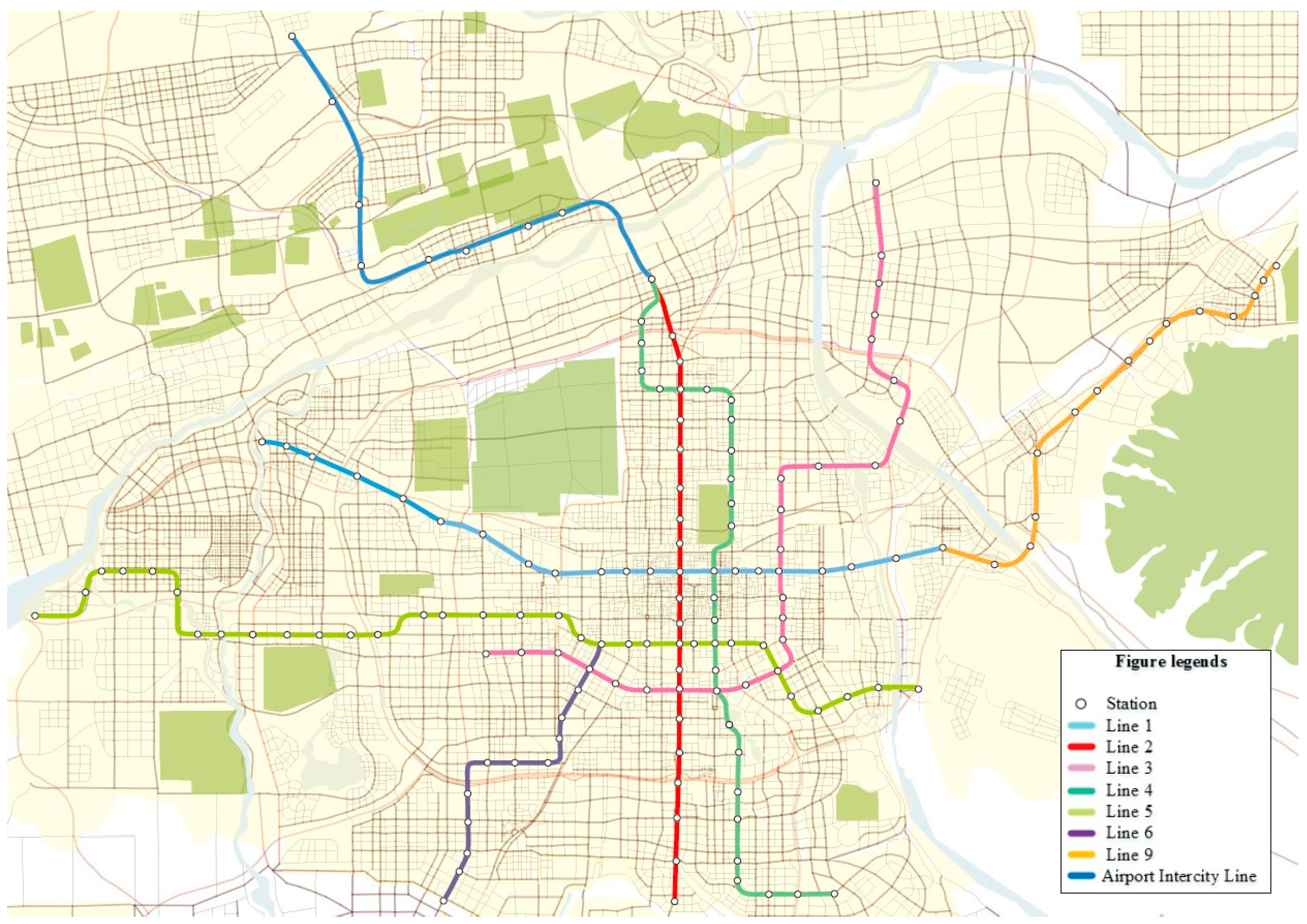
Xi’an, the first city to operate an urban rail transit system in Northwest China, was selected as the case study area. As of May 2021, Xi’an had a rail transit system in operation with 244 km, 8 lines, and 153 stations, as shown in Figure 1.
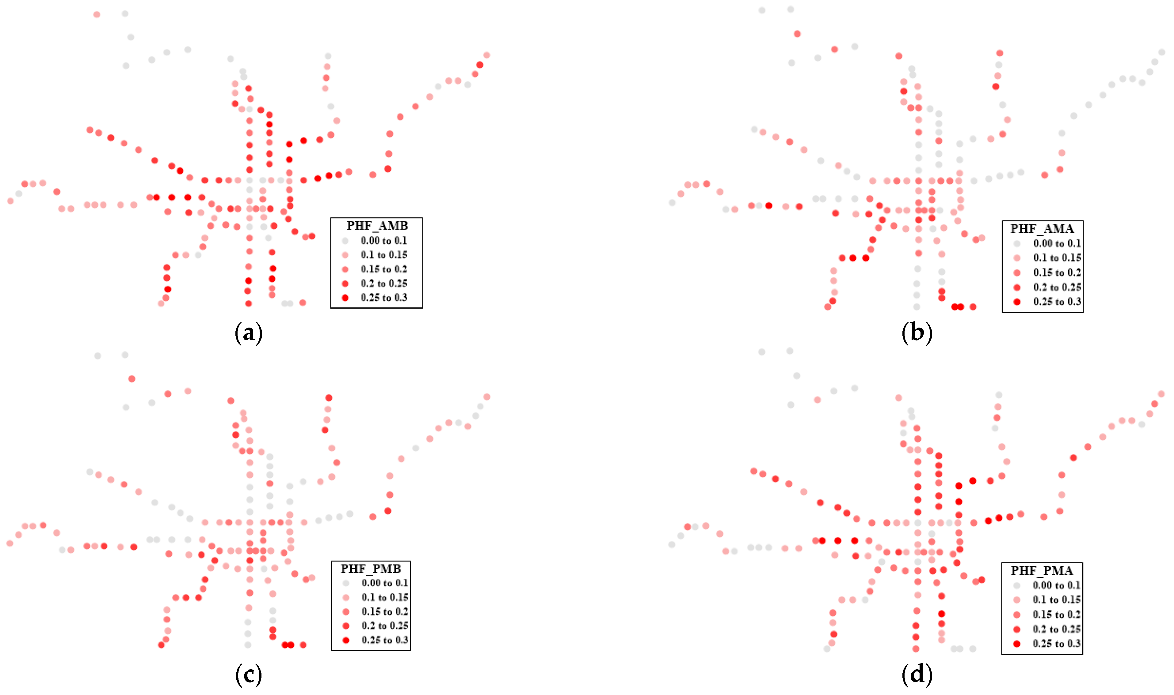
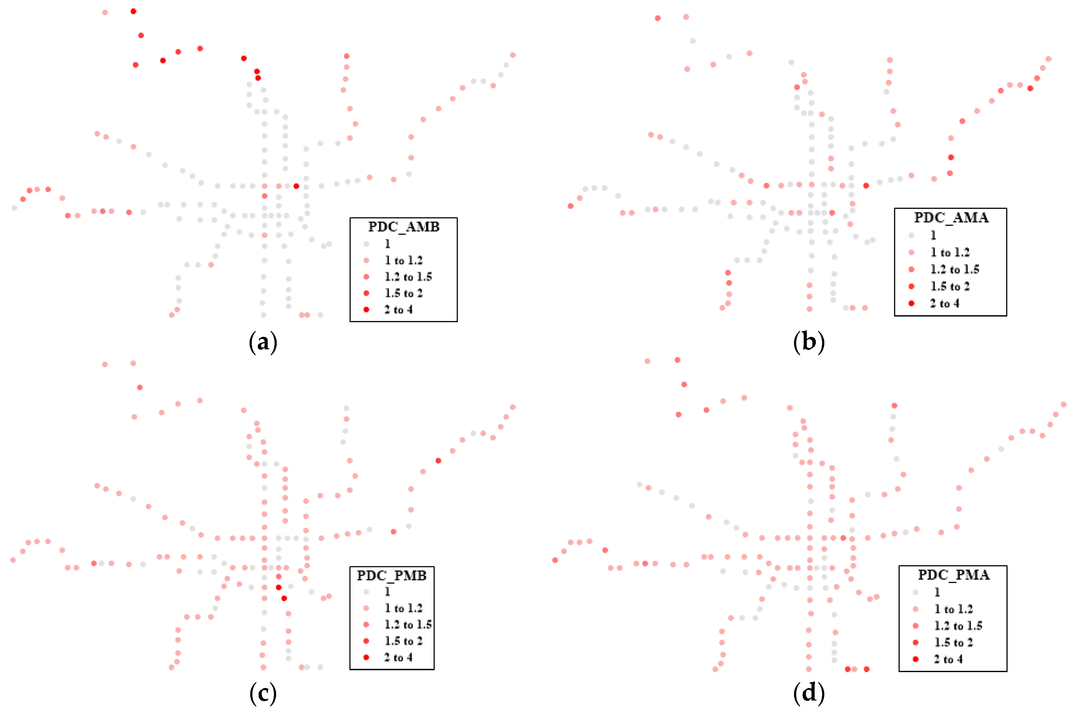
The historical subway ridership data were aggregated at 15 min intervals from smart card data acquired from the Xi’an Metro company, constituting a general dataset from 17–21 May 2021. The station ridership peaks in this study were subdivided into four types, including the morning boarding ridership peak (AMB), morning alighting ridership peak (AMA), evening boarding ridership peak (PMB), and evening alighting ridership peak (PMA). Accordingly, four PHFs (PHF_AMB, PHF_AMA, PHF_PMB, PHF_PMA) and four PDCs (PDC_AMB, PDC_AMA, PDC_PMB, PDC_PMA) corresponding to the four distinct peak periods were, respectively, calculated by Equations (2) and (3). These values were averaged across weekdays and set as dependent variables with the total sample size of 153 × 8 in the model input.
As for the data associated with dependent variables, POI data within the catchment areas were collected from Baidu Map with the assistance of API, based on which the land-use entropy was calculated using Equation (4). Regarding the station characteristic variables, the operating time was sourced from the official website of the Xi’an Rail Transit Group Company, Ltd., and the distance to the city center and betweenness centrality were calculated with the assistance of Baidu Maps. The data related to the accessibility variables were collected from Baidu Maps and calculated based on the Geographical Information System (GIS) spatial analysis tools.
The pedestrian catchment areas of subway stations should first be evaluated before collecting the data, such as land-use variables and station characteristics, aiming to determine the range of data collection. According to previous studies [25,26,27,28,29], a distance of 800 m was considered as the standard walking distance to delineate the pedestrian catchment areas of subway stations. The Thiessen polygon was used to deal with the possible buffer overlaps between some stations [30].
3.1.2. Data Preprocessing Results
Figure 2 and Figure 3 intuitively present the spatial distributions of the four types of PHF and PDC values of the existing 153 stations, respectively. A considerable number of stations had PDC values greater than 1 or that even exceeded 2 at certain peak periods, which indicates that the peak deviation phenomenon significantly exists in the subway stations in the case study. Moreover, the distribution of both the PHF and PDC exhibited spatial correlation and aggregation to a certain extent. Specifically, for the morning peaks, stations with a large PHF were found to be relatively concentrated in the city region in the boarding direction and densely clustered in the city center and southwest regions in the alighting direction, while this situation was the reverse for the evening peaks. Peak deviation was inclined to arise in stations peripheral to the city, especially during morning peak periods, and the ridership deviation magnitude was found to be generally positively associated with the distance from the station to the city center to some extent.
Table 1 displays the main descriptive statistics of the candidate independent variables of the PHF and PDC models.
3.2. PHF and PDC Estimation Result Analysis
3.2.1. Model Comparisons
Before the model was established, Moran’s I index was utilized to detect the spatial correlation of the dependent and candidate-independent variables. The results show that statistically significant spatial autocorrelation at the 1% level was identified for all dependent and candidate-independent variables. Then, the independent variables were retained in the PHF and PDC models selected by LASSO. All variables were adopted as their natural logarithm to reduce potential heteroscedasticity during model input. It can be seen that between 8 and 14 key PHF and PDC predictors were identified, as shown in Table 2.
3.2.2. PHF Estimation Results and Interpretation
Table 3 reports the estimation results of the PHF for the SDM. In general, the living services had the largest impact magnitude across all types of peak periods, but the impact direction differed in different peak periods. Specifically, a positive influence was generated in boarding ridership, and a negative influence was generated in alighting ridership for morning peak hours, which was reversed for evening peak hours. This largely reflects the trip pattern of resident commuters, implying that station-area living services are highly important in cultivating commuter residency, and this, in turn, may increase commuting trips.
The estimation coefficients of the other variables generally varied with the peak periods, and thus, the dominant factors differed in different peak periods. For morning peak hours, the distance to the city center, transport facilities, and residences had the highest impact magnitudes in the boarding direction, but their impact directions differed. The residences around the station contributed to the increase in ridership, while the long distance to the city center and transport facilities contributed to mitigating the burden of the peak ridership. Regarding the alighting ridership, offices, restaurants, and road density were found to generate the largest and most positive influences, indicating that more offices, more restaurants, and higher road density may effectively attract “working-purpose” trips. For evening peak periods, offices, the distance to the city center, and the road density generated the largest and most positive influences on boarding ridership. This finding seems to be related to the fact that residences and offices are not effectively integrated. A long commuting distance or high connection accessibility compels commuters to be more inclined to choose the subway as their main commuting mode. Regarding alighting ridership, retailers and transport facilities were found to play a dominating role in easing concentrated alighting demand in peak hours. This implies that passengers with the purpose of shopping or accessing transportation hubs are inclined to travel within off-peak periods, as they have a relatively flexible travel schedule.
Regarding the spatial neighboring effects, healthcare facilities, living services, and operation time were found to have significant influences in all types of peak periods. Specifically, healthcare facilities generated a positive influence, indicating that an increase in the healthcare facilities of the surrounding stations might promote the overall travel demand. The living services and operation time generated a positive influence for morning boarding and evening alighting peak ridership but a negative influence for morning alighting and evening boarding peak ridership; this indicates that the living services of neighboring stations may attract resident commuters, which, in turn, promotes go-to-work trips. The impact magnitudes of other significant spatial lag variables differed in the four peak periods. In terms of morning peak hours, schools generated the largest positive influence, and hotels generated the largest negative influence in the boarding direction. Offices and the distance to the city center, respectively, generated the largest positive and negative influences on the PHF for the alighting direction. Regarding evening peak hours, the road density and land-use entropy, respectively, generated the largest positive and negative influences in the boarding direction, while the operation time and transport facilities, respectively, generated the largest positive and negative influences in the alighting direction. In addition, the coefficients of the spatial lag variable (WY) indicate that a spatial spillover effect existed in the PHF in all four peak periods.
3.2.3. PDC Estimation Results and Interpretation
Table 4 reports the estimation results of the PDC for the SDM. In general, retailers, healthcare facilities, and the operation time were found to have significant effects regardless of the peak period. This suggests that the allocation of retailers and healthcare facilities is the key to avoiding the risks posed by the deviation in station ridership peaks and must therefore be prudently planned. Specifically, the influence of retailers was negative for the morning boarding and evening alighting peak periods and positive for the morning alighting and evening boarding peak periods, while the influence of the operation time was reversed. The impact of healthcare facilities was negative in the boarding direction peaks, while it was positive in the alighting direction peaks.
The estimation coefficients of individual variables generally varied with the peak periods, and the dominant factors differed in the four peak periods. For morning peak periods, transport facilities were found to have a dominant role in peak deviation, while residential units were a key factor that mitigated the magnitude of peak deviations in the boarding direction. Regarding the alighting direction, the distance to the city center had the largest and most positive impact, indicating that suburban stations are more prone to attracting irregular “non-commuting purpose” trips because the majority of jobs and schools are generally located in or close to the city center. Offices had the largest and most negative impact, indicating that offices are crucial for avoiding the risk of alighting ridership deviation, as “working-purpose” trips generally have fixed and consistent commuting times. For evening peak periods, residences and land-use entropy, respectively, played a dominating role in mitigating and contributing peak deviation in the boarding direction. In terms of the alighting direction, the land-use entropy and the number of bus lines played a dominant role in mitigating the magnitude of peak deviations. This implies that reasonable land resource allocation and good connection accessibility are more likely to attract resident commuters, and this, in turn, contributes to the generation of regular travel.
Concerning the spatial neighboring effects, retailers, healthcare facilities, and operation time were found to have significant influences in all types of peak periods. Healthcare facilities generated a negative influence in the boarding direction, whereas they had a positive influence in the alighting direction. Retailers and the operation time generated a negative influence during the morning boarding and evening alighting peak periods but a positive influence during the morning alighting and evening boarding peak periods; this indicates that commuters are more prone to reside near stations with strong commerce or a long operation time, and this, in turn, contributes to avoiding the risk of peak deviation due to the considerably regular “go-to-work” trips generated. Regarding the other significant spatial lag variables, their impact magnitudes differed in the four peak periods. In terms of morning peak hours, transport facilities and offices, respectively, generated the largest positive and negative influences in the boarding direction, and the road density and retailers generated the largest and most positive influences in the alighting direction. Regarding evening peak hours, the land-use entropy and the number of bus lines, respectively, generated the largest positive and negative influences in the boarding direction, while the land-use entropy and restaurants generated the largest and most negative influences in the alighting direction. In addition, tourist spots had an obvious negative effect on the PDC in the alighting direction, which is indicative of the fact that individuals traveling for “tourism purposes” are inclined to avoid rush hours, as they have a relatively flexible schedule. The coefficients of the spatial lag variable (WY) indicate that a spatial spillover effect existed in the PDC in all four peak periods.
3.2.4. SPR Estimation Results Analysis
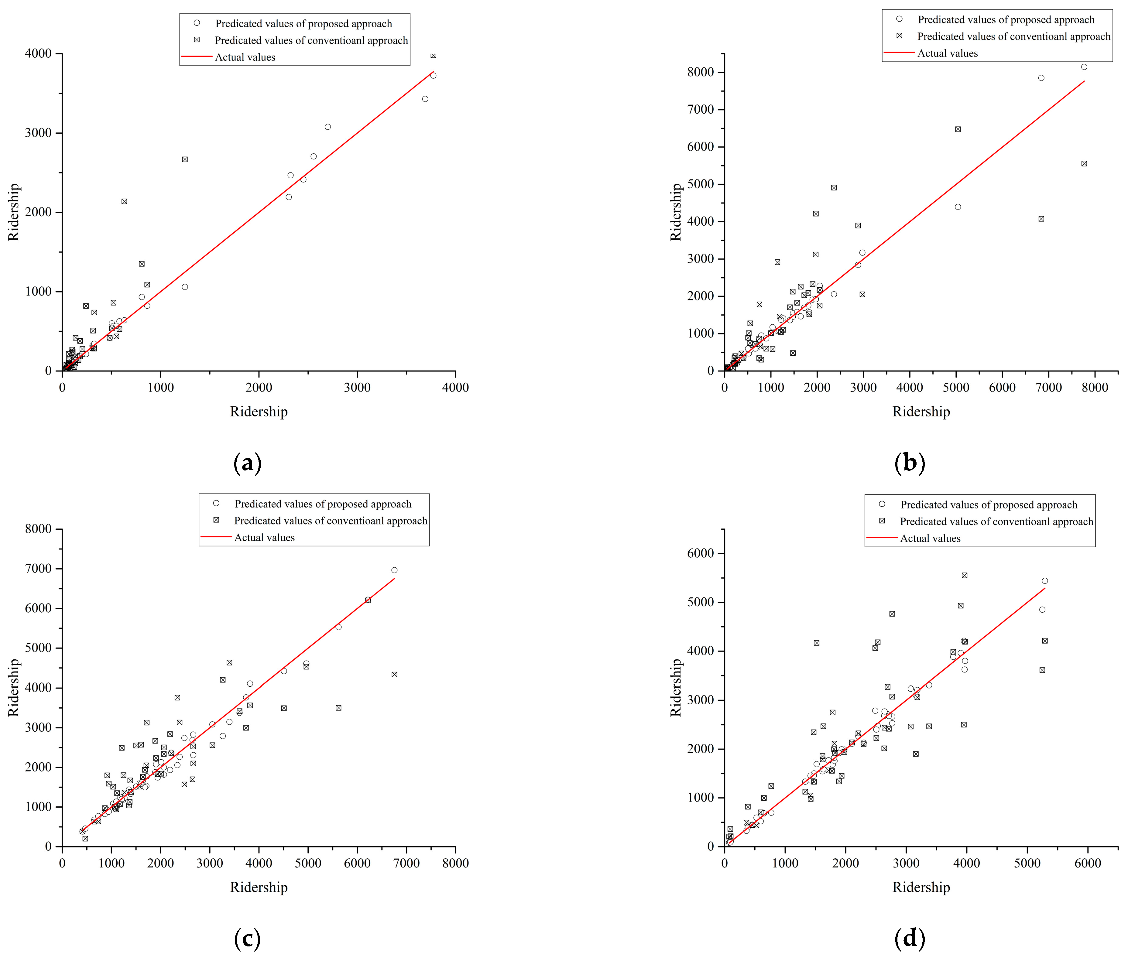
Relying on the constructed PHF and PDC spatial relationship models produced by the SDM, the SPR values were computed according to Equation (13). The results are shown in Figure 4. To examine the performance of the proposed approach, the mean absolute percentage error (MAPE) was computed, as shown in Table 5. The MAPE values of the proposed approach fell between 0.096 and 0.194, demonstrating excellent prediction precision. The proposed approach achieved a decrease in the MAPE value of 0.158–0.396 compared to the traditional approach (four-step methods [6,31]), indicating a significant improvement in the prediction accuracy. It can be seen that the traditional approach exhibited poor applicability with the MAPE value, reaching 0.590 during the morning boarding peak period. By comparison, the proposed approach exhibited significant superiority in terms of estimation errors and performance stability. These pieces of evidence demonstrate that the proposed approach exhibits wider applicability and higher estimation accuracy for SPR estimation.
4. Discussion and Conclusions
This study proposed a comprehensive and refined framework for SPR estimation that can simultaneously accommodate the scenarios of stations with peak consistency and peak deviation. The proposed framework introduces the PDC to calibrate the SPR estimation results of peak deviation stations and employs a spatial regression model, namely the SDM, to model and determine the two key parameters in the SPR estimation process (i.e., the PHF and PDC). The empirical results demonstrate the wider applicability and higher estimation accuracy of the proposed approach.
The construction of the subway would increase the inequity of the city [32], forcing the government to make more residents enjoy subway travel by increasing feeder buses or raising land-use construction around stations. This presents a challenge for planning authorities, namely how to achieve the optimal allocation of land-use attributes along subway lines. The land generating commuter flow makes the peak sharp, while the land generating life travel makes the peak inconsistent with the lines’ peak. The PHF and the PDC reflect the time aggregation characteristics of station-level ridership from two aspects, meaning the aggregation and deviation of peaks. The results show that land-use attributes that greatly influence the two parameters have opposite signs, revealing that the same property of the land can only cause the ridership to exhibit one of the aggregation or deviation phenomena. The better estimation results of the spatial model imply that the PHF and PDC of a station are also influenced by the attributes of its neighbors. Thus, when planning the land around stations, we need to balance different types of land, reducing the ridership peak value and preventing the peak deviation at the same time.
Regarding land use, morning boarding and evening alighting can be recognized as a group, while morning alighting and evening boarding can be considered another group. The fitting results of most factors to PHF have the same plus and minus signs in the same group, while they have different plus and minus signs in different groups. This indicates that these lands contribute to forming the commuter flow and have opposite influences on the generation or attraction in the peak hour. However, the fitting results of PDC do not have this regularity, implying the disorder of non-commuting travel. In the morning peak hour, living services, residences, and healthcare are the main sources of generation, and restaurants and finance spots are the main sources of attraction. The regression coefficients of PHF in these two groups have the opposite law of positive and negative effects, but the coefficients of PDC are negative influences. The impacts on PHF of retailers are negative both in boarding and alighting, suggesting that this land does not produce commuter traffic, and its PDCs in boarding and alighting are diverse. However, schools have little influence on PHF, this may be related to the policy of attending a designated primary school belonging to the living location issued by the Chinese government, which reduced the travel distance of attending school. Thus, planners can use these results to balance the peak and off-peak travel demands to improve the operating efficiency of subway lines.
The distance to the city center has a highly positive influence on PHF in morning alighting and evening boarding, while it has a highly negative influence on PDC in morning boarding and evening alighting and a highly positive influence in morning alighting. This finding seems to be related to the fact that the Xi’an city skeleton enlarged and the travel distance lengthened with the relocation of its government from the city center to the north, the maturity of the high-tech industrial area in the southwest, and the education area in the south.
Furthermore, the SDM enables the underlying spatial influencing mechanisms of the PHF and PDC to be revealed, which provides a theoretical reference for decision-makers to prudently deploy land-use resources while incorporating a spatial perspective, thereby balancing the travel demand between peak and off-peak periods and thus improving the line operation efficiency.
However, this study was characterized by some limitations. For instance, more related influencing factors should be considered in the PHF and PDC models if the data are available. Moreover, the spatial model performance will be further improved by constructing more complicated schemes of the spatial weight matrix [33].
Author Contributions
Conceptualization, Y.Z. and J.W.; Methodology, Y.Z. and J.W.; Software, Y.Z. and J.W.; Formal analysis, Y.Z. and J.W.; Investigation, Y.Z.; Writing—original draft, Y.Z.; Writing—review and editing, J.W., H.L. and Y.H.; Visualization, Y.Z.; Supervision, J.W., H.L. and Y.H. All authors have read and agreed to the published version of the manuscript.
Funding
This work was jointly supported by the Key Research and Development Project of Gansu Provincial Science and Technology Department (22YF7GA142) and the Systematic Major Project of China National Railway Group (P2021S012).
Data Availability Statement
Data are available on request due to restrictions. The data presented in this study are available on request from the corresponding author. The data are not publicly available due to data protection or privacy concerns.
Conflicts of Interest
The authors declare no conflict of interest.
References
- Wang, J.; Li, Y.; Jiao, J.; Jin, H.; Du, F. Bus ridership and its determinants in Beijing: A spatial econometric perspective. Transportation 2022, 50, 383–406. [Google Scholar] [CrossRef]
- Wu, P.; Chen, T.; Wong, Y.D.; Meng, X.; Wang, X.; Liu, W. Exploring key spatio-temporal features of crash risk hot spots on urban road network: A machine learning approach. Transp. Res. Part A Policy Pract. 2023, 173, 103717. [Google Scholar] [CrossRef]
- Li, G.; Wu, J.; He, Y.; Li, D. CQDFormer: Cyclic quasi-dynamic transformers for hourly origin-destination estimation. Appl. Sci. 2023, 13, 11257. [Google Scholar] [CrossRef]
- Ahad, A.P.; Yang, Q.; Zhang, S.; Pishro, M.A.; Zhang, Z.; Zhao, Y.; Postel, V.; Huang, D.; Li, W. Node, place, ridership, and time model for rail-transit stations: A case study. Sci. Rep. 2022, 12, 16120. [Google Scholar] [CrossRef]
- Pan, P.; Wang, H.; Li, L.; Wang, Y.; Jin, Y. Peak-hour subway passenger flow forecasting: A tensor based approach. In Proceedings of the 21st International Conference on Intelligent Transportation Systems (ITSC), Maui, HI, USA, 4–7 November 2018. [Google Scholar] [CrossRef]
- Liu, J.; Ma, X.; Liu, C.; Wang, Y.; Wang, J. Temporal distribution analysis of Beijing’s subway ridership. In Proceedings of the 16th COTA International Conference of Transportation Professionals, Shanghai, China, 6–9 July 2016. [Google Scholar] [CrossRef]
- Wei, J.; Cheng, Y.; Chen, K.; Wang, M.; Ma, C.; Hu, X. Nonlinear model-based subway station-level peak-hour ridership estimation approach in the context of peak deviation. Transp. Res. Rec. 2022, 2676, 549–564. [Google Scholar] [CrossRef]
- Chen, K.; Yu, L.; Ma, C. Differentiated peak hours at urban rail transit stations in Xi’an. Urban Transp. China 2018, 16, 51–58. [Google Scholar] [CrossRef]
- Gu, L.; Ye, X. Research on peak time of passenger flow entering and leaving stations in Osaka rail transit stations. Compr. Transp. China 2014, 2, 57–61. [Google Scholar]
- Yu, L.; Chen, Q.; Chen, K. Deviation of peak hours for urban rail transit stations: A case study in Xi’an, China. Sustainability 2019, 11, 2733. [Google Scholar] [CrossRef]
- Park, Y.; Choi, Y.; Kim, K.; Yoo, J.K. Machine learning approach for study on subway passenger flow. Sci. Rep. 2022, 12, 2754. [Google Scholar] [CrossRef]
- Zhong, C.; Batty, M.; Manley, E.; Wang, J.; Wang, Z.; Chen, F.; Schmitt, G. Variability in regularity: Mining temporal mobility patterns in London, Singapore and Beijing using smart-card data. PLoS ONE 2016, 11, e0149222. [Google Scholar] [CrossRef] [PubMed]
- Lee, J.; Boarnet, M.; Houston, D.; Nixon, H.; Spears, S. Changes in service and associated ridership impacts near a new light Rail transit line. Sustainability 2017, 9, 1827. [Google Scholar] [CrossRef]
- Shantz, A.; Casello, J.; Woudsma, C.; Guerra, E. Understanding factors associated with commuter rail ridership: A demand elasticity study of the GO transit rail network. Transp. Res. Rec. 2022, 2676, 131–143. [Google Scholar] [CrossRef]
- Yu, L.; Cong, Y.; Chen, K. Determination of the peak hour ridership of metro stations in Xi’an, China using geographically- weighted regression. Sustainability 2020, 12, 2255. [Google Scholar] [CrossRef]
- Wei, J.; Cheng, Y.; Yu, L.; Zhang, S.; Chen, K. Improved approach for forecasting extra-peak hourly subway ridership at station-level based on LASSO. J. Transp. Eng. Part A Syst. 2021, 147, 4021079. [Google Scholar] [CrossRef]
- Liu, S.; Yao, E.; Li, B. Exploring urban rail transit station-level ridership growth with network expansion. Transp. Res. Part D Transp. Environ. 2018, 73, 391–402. [Google Scholar] [CrossRef]
- Zhao, X.; Wu, Y.; Ren, G.; Ji, K.; Qian, W. Clustering analysis of ridership patterns at subway stations: A case in Nanjing, China. J. Urban Plan. Dev. 2019, 145, 04019005. [Google Scholar] [CrossRef]
- Feng, X.; Sun, Q.; Liu, J.; Yang, Y.; Liang, X. Time characteristic of input passenger in urban rail transit stations among high density residential areas. In Proceedings of the 29th Chinese Control Conference, Beijing, China, 29–31 July 2010. [Google Scholar]
- Yu, J. Characteristics of peak hour passenger flow at rail transit stations in Shanghai. Urban Transp. China 2019, 17, 50–57. [Google Scholar] [CrossRef]
- Wang, J.; Yamamoto, T.; Liu, K. Spatial dependence and spillover effects in customized bus demand: Empirical evidence using spatial dynamic panel models. Transp. Policy 2021, 105, 166–180. [Google Scholar] [CrossRef]
- Zhu, P.; Huang, J.; Wang, J.; Liu, Y.; Li, J.; Wang, M.; Qiang, W. Understanding taxi ridership with spatial spillover effects and temporal dynamics. Cities 2022, 125, 103637. [Google Scholar] [CrossRef]
- Kong, X.; Yang, J. A new method for forecasting station-level transit ridership from land-use perspective: The case of Shenzhen city. Sci. Geogr. Sin. 2018, 38, 2074–2083. [Google Scholar] [CrossRef]
- Jiao, J.; Wang, J.; Zhang, F.; Jin, F.; Liu, W. Roles of accessibility, connectivity and spatial interdependence in realizing the economic impact of high-speed rail: Evidence from China. Transp. Policy 2020, 91, 1–15. [Google Scholar] [CrossRef]
- Wang, H.; Cui, H.; Zhao, Q. Effect of green technology innovation on green total factor productivity in China: Evidence from spatial durbin model analysis. J. Clean. Prod. 2020, 288, 125624. [Google Scholar] [CrossRef]
- Anselin, L. Spatial Econometrics: Methods and Models; Springer: Dordrecht, The Netherlands, 1998. [Google Scholar]
- Sung, H.; Oh, J. Transit-oriented development in a high-density city: Identifying its association with transit ridership in Seoul, Korea. Cities 2011, 28, 70–82. [Google Scholar] [CrossRef]
- Cardozo, O.D.; García-Palomares, J.C.; Javier, G. Application of geographically weighted regression to the direct forecasting of transit ridership at station-level. Appl. Geogr. 2012, 34, 548–558. [Google Scholar] [CrossRef]
- Zhao, J.; Deng, W.; Yan, S.; Zhu, Y. What influences metro station ridership in China? insights from Nanjing. Cities 2013, 35, 114–124. [Google Scholar] [CrossRef]
- Li, S.; Lyu, D.; Huang, G.; Zhang, X.; Gao, F.; Chen, Y.; Liu, X. Spatially varying impacts of built environment factors on rail transit ridership at station level: A case study in Guangzhou, China. J. Transp. Geogr. 2020, 82, 102631. [Google Scholar] [CrossRef]
- Wang, J.; Liu, J.; Ma, Y.; Sun, F.; Chen, F. Temporal and spatial passenger flow distribution characteristics at rail transit stations in Beijing. Urban Transp. China 2013, 11, 18–27. [Google Scholar] [CrossRef]
- Yu, L.; Cui, M. How subway network affects transit accessibility and equity: A case study of Xi’an metropolitan area. J. Transp. Geogr. 2023, 108, 103556. [Google Scholar] [CrossRef]
- Lu, J.; Zhang, L. Modeling and prediction of tree height diameter relationships using spatial autoregressive models. For. Sci. 2011, 57, 252–264. [Google Scholar] [CrossRef]
Figure 1.
Spatial distribution of stations in the case study area.

Figure 2.
Spatial distribution of PHF. (a) AMB. (b) AMA. (c) PMB. (d) PMA.

Figure 3.
Spatial distribution of PDC. (a) AMB. (b) AMA. (c) PMB. (d) PMA.

Figure 4.
Comparison of the SPR values in the traditional approach and proposed approach. (a) AMB. (b) AMA. (c) PMB. (d) PMA.
Figure 4.
Comparison of the SPR values in the traditional approach and proposed approach. (a) AMB. (b) AMA. (c) PMB. (d) PMA.


Table 1.
Descriptive statistics of candidate independent variables.
| Categories | Independent Variables | Notation | Mean | Min. | Max. |
|---|---|---|---|---|---|
| Land use | Number of residences | 46 | 0 | 177 | |
| Number of offices | 128 | 1 | 1084 | ||
| Number of government organizations | 42 | 0 | 210 | ||
| Number of restaurants | 324 | 0 | 1344 | ||
| Number of retailers | 451 | 0 | 2762 | ||
| Number of schools | 82 | 0 | 326 | ||
| Number of healthcare | 61 | 0 | 193 | ||
| Number of transport facilities | 72 | 2 | 222 | ||
| Number of tourist spots | 8 | 0 | 123 | ||
| Number of finance spots | 23 | 0 | 101 | ||
| Number of living services | 329 | 0 | 1577 | ||
| Number of hotels | 78 | 0 | 820 | ||
| Land-use entropy | 0.78 | 0.41 | 0.89 | ||
| Station characteristics | Distance to city center (km) | 10.65 | 0.24 | 30.6 | |
| Betweenness centrality | 0.1 | 0 | 0.48 | ||
| Operating time (year) | 3.5 | 0.38 | 9.67 | ||
| Accessibility | Number of bus lines | 55 | 1 | 169 | |
| Road density (km/km2) | 3.43 | 0.93 | 9.07 |
Table 2.
Model performance comparison of PHF and PDC estimation based on testing set.
| Peak Types | Evaluation Indexes | PHF | PDC | ||||||
|---|---|---|---|---|---|---|---|---|---|
| OLS | SLM | SEM | SDM | OLS | SLM | SEM | SDM | ||
| AMB | AIC | −418.56 | −457.59 | −471.74 | −489.32 | 157.16 | 145.77 | 132.43 | 89.214 |
| LRT | 0.11 | 14.26 | 23.34 | 1.58 | 12.91 | 14.43 | |||
| AMA | AIC | −411.37 | −423.98 | −418.06 | −448.44 | −221.34 | −224.39 | −222.56 | −227.61 |
| LRT | 15.34 | 17.42 | 19.22 | 0.01 | 3.18 | 4.64 | |||
| PMB | AIC | −524.39 | −541.43 | −537.61 | −583.67 | −177.36 | −181 | −180.52 | −188.5 |
| LRT | 8.89 | 10.07 | 13.72 | 0.53 | 0.06 | 3.1 | |||
| PMA | AIC | −613.59 | −642.75 | −657.69 | −678.4 | −234.97 | −253.29 | −258.61 | −347.09 |
| LRT | 2.23 | 17.17 | 20.49 | 0.36 | 5.68 | 7.51 | |||
1. The first longitudinal term “AMB, AMA, PMB, PMA” denotes four types of peaks, corresponding to the morning boarding ridership peak (AMB), morning alighting ridership peak (AMA), evening boarding ridership peak (PMB), and evening alighting ridership peak (PMA), respectively; 2. The second longitudinal term “AIC, LRT” denotes two evaluation indexes, namely the Akaike Information Criterion (AIC) and Likelihood Ratio Test (LRT); 3. The second transverse term “OSL, SLM, SEM, SDM” denotes four methods, namely ordinary least squares (OSL), spatial lag model (SLM), spatial error model (SEM), and spatial Durbin model (SDM).
Table 3.
PHF estimation results of SDM.
| Variables | AMB | AMA | PMB | PMA | ||||
|---|---|---|---|---|---|---|---|---|
| X | WX | X | WX | X | WX | X | WX | |
| 0.0205 * | −0.0026 | −0.0022 * | −0.0056 | — | — | — | — | |
| 0.0020 * | −0.0047 | 0.0332 *** | 0.0184 | 0.0203 *** | 0.0134 | — | — | |
| — | — | 0.0004 * | 0.0010 | — | — | −0.0022 * | −0.0037 | |
| −0.0189 *** | 0.0024 | 0.0236 *** | −0.0041 | — | — | — | — | |
| −0.0056 * | −0.0082 | −0.0148 *** | −0.0071 | — | — | −0.0061 * | −0.0020 | |
| −0.0110 * | 0.0076 | — | — | — | — | — | — | |
| 0.0198 *** | 0.0071 | −0.0110 * | 0.0167 | −0.0026 * | 0.0088 | 0.0049 * | 0.0005 | |
| −0.0216 *** | −0.0081 | 0.0107 * | 0.0035 | — | — | −0.0079 * | −0.0075 | |
| — | — | — | — | — | — | 0.0007 * | 0.0010 | |
| −0.0137 *** | −0.0081 | 0.0130 *** | 0.0032 | — | — | −0.0041 * | −0.0026 | |
| 0.0498 *** | 0.0213 | −0.0502 *** | −0.0262 | −0.0242 *** | −0.0239 | 0.0226 *** | 0.0139 | |
| 0.0007 * | −0.0103 | −0.0091 * | 0.0059 | −0.0020 * | 0.0052 | — | — | |
| — | — | — | — | 0.0009 * | −0.0142 | — | — | |
| — | — | 0.0177 * | 0.0138 | 0.0130 * | 0.0150 | 0.0010 * | −0.0074 | |
| — | — | — | — | — | — | −0.0036 * | −0.0023 | |
| −0.0054 * | 0.0031 | 0.0098 * | −0.0053 | 0.0007 * | −0.0009 | −0.0030 * | 0.0014 | |
| −0.0277 * | 0.0026 | 0.0115 * | −0.0088 | 0.0108 * | −0.0008 | — | — | |
| 0.0008 * | 0.0042 | −0.0063 * | −0.0008 | — | — | — | — | |
| — | −0.0144 | — | 0.0377 | — | −0.0044 | — | 0.0038 | |
| 0.1504 | — | 0.0874 | — | 0.0936 | — | 0.0511 | — | |
1. The first transverse term “AMB, AMA, PMB, PMA” denotes four types of peaks, corresponding to the morning boarding ridership peak (AMB), morning alighting ridership peak (AMA), evening boarding ridership peak (PMB), and evening alighting ridership peak (PMA), respectively; 2. The second transverse term “X, WX” denotes the direct effects and indirect effects of independent variables, respectively; 3. * means that the variable is retained in the model; ***, and * indicate significant levels at 1% and 10%, respectively; 4. The prefix “ln” before the explanatory variables denotes a logarithmic form.
Table 4.
PDC estimation results of SDM.
| Variables | AMB | AMA | PMB | PMA | ||||
|---|---|---|---|---|---|---|---|---|
| X | WX | X | WX | X | WX | X | WX | |
| −0.1243 *** | −0.0291 | — | — | −0.0457 *** | 0.0159 | — | — | |
| −0.0591 *** | −0.0824 | −0.0302 *** | −0.0123 | — | — | — | — | |
| — | — | 0.0187 * | 0.0093 | — | — | 0.0221 *** | 0.0048 | |
| — | — | — | — | — | — | −0.0291 *** | −0.0327 | |
| −0.0194 * | −0.0001 | 0.0050 * | 0.0124 | 0.0403 *** | 0.0139 | −0.0362 *** | −0.0196 | |
| — | — | −0.0080 * | −0.0060 | −0.0109 * | 0.0126 | 0.0339 *** | −0.0118 | |
| −0.0171 * | −0.0718 | 0.0277 * | 0.0117 | −0.0297 * | −0.0220 | 0.0116 * | 0.0147 | |
| 0.1138 *** | 0.2327 | — | — | — | — | — | — | |
| −0.0234 * | −0.0289 | 0.0014 * | −0.0062 | — | — | 0.0005 * | 0.0019 | |
| −0.0351 | 0.0384 | −0.0215 * | −0.0030 | — | — | 0.0154 * | 0.0062 | |
| — | — | — | — | — | — | −0.0207 * | 0.0237 | |
| — | — | — | — | −0.0026 | −0.0032 | 0.0143 ** | 0.0053 | |
| — | — | — | — | 0.3102 *** | 0.1253 | −0.3938 *** | −0.1643 | |
| −0.0182 * | −0.0648 | 0.0157 * | 0.0198 | — | — | −0.0281 * | 0.0083 | |
| — | — | — | — | 0.0073 * | −0.0246 | −0.0452 *** | 0.0212 | |
| 0.0303 * | −0.0002 | −0.0169 * | 0.0016 | −0.0063 * | 0.0053 | 0.0116 * | −0.0076 | |
| — | — | 0.0743 * | 0.0006 | — | — | — | — | |
| — | — | 0.0093 * | −0.0031 | 0.0055 * | −0.0014 | 0.0086 * | −0.0057 | |
| — | −0.2560 | — | −0.1042 | — | 0.0263 | — | −0.0575 | |
| 1.8264 | — | 1.0102 | — | 1.0299 | — | 1.3434 | — | |
1. The first transverse term “AMB, AMA, PMB, PMA” denotes four types of peaks, corresponding to the morning boarding ridership peak (AMB), morning alighting ridership peak (AMA), evening boarding ridership peak (PMB), and evening alighting ridership peak (PMA), respectively; 2. The second transverse term “X, WX” denotes the direct effects and indirect effects of independent variables, respectively; 3. * means that the variable is retained in the model; ***, **, and * indicate significant levels at 1%, 5%, and 10%, respectively; 4. The prefix “ln” before the explanatory variables denotes a logarithmic form.
Table 5.
The MAPE of SPR.
| MAPE | AMB | AMA | PMB | PMA |
|---|---|---|---|---|
| Traditional approach | 0.590 | 0.377 | 0.255 | 0.324 |
| Proposed approach | 0.194 | 0.118 | 0.097 | 0.096 |
| Decreased value | 0.396 | 0.259 | 0.158 | 0.228 |
Disclaimer/Publisher’s Note: The statements, opinions and data contained in all publications are solely those of the individual author(s) and contributor(s) and not of MDPI and/or the editor(s). MDPI and/or the editor(s) disclaim responsibility for any injury to people or property resulting from any ideas, methods, instructions or products referred to in the content. |
© 2024 by the authors. Licensee MDPI, Basel, Switzerland. This article is an open access article distributed under the terms and conditions of the Creative Commons Attribution (CC BY) license (https://creativecommons.org/licenses/by/4.0/).
Share and Cite
MDPI and ACS Style
Zhao, Y.; Wei, J.; Li, H.; Huang, Y. Predicting Station-Level Peak Hour Ridership of Metro Considering the Peak Deviation Coefficient. Sustainability 2024, 16, 1225. https://0-doi-org.brum.beds.ac.uk/10.3390/su16031225
AMA Style
Zhao Y, Wei J, Li H, Huang Y. Predicting Station-Level Peak Hour Ridership of Metro Considering the Peak Deviation Coefficient. Sustainability. 2024; 16(3):1225. https://0-doi-org.brum.beds.ac.uk/10.3390/su16031225
Chicago/Turabian StyleZhao, Ying, Jie Wei, Haijun Li, and Yan Huang. 2024. "Predicting Station-Level Peak Hour Ridership of Metro Considering the Peak Deviation Coefficient" Sustainability 16, no. 3: 1225. https://0-doi-org.brum.beds.ac.uk/10.3390/su16031225
Note that from the first issue of 2016, this journal uses article numbers instead of page numbers. See further details here.