Article

Comparative Evaluation of Crash Hotspot Identification Methods: Empirical Bayes vs. Potential for Safety Improvement Using Variants of Negative Binomial Models

1
UGent, Department of Civil Engineering, Technologiepark 60, 9052 Zwijnaarde, Belgium
2
UHasselt, Transportation Research Institute (IMOB), Martelarenlaan 42, 3500 Hasselt, Belgium
3
UHasselt, Faculty of Engineering Technology, Agoralaan, 3590 Diepenbeek, Belgium
*
Author to whom correspondence should be addressed.
Sustainability 2024, 16(4), 1537; https://0-doi-org.brum.beds.ac.uk/10.3390/su16041537
Submission received: 22 January 2024 / Revised: 6 February 2024 / Accepted: 8 February 2024 / Published: 11 February 2024
(This article belongs to the Collection Emerging Technologies and Sustainable Road Safety)

Abstract

:
The empirical Bayes (EB) method is widely acclaimed for crash hotspot identification (HSID), which integrates crash prediction model estimates and observed crash frequency to compute the expected crash frequency of a site. The traditional negative binomial (NB) models, often used to estimate crash predictive models, typically struggle with accounting for the unobserved heterogeneity in crash data. Complex extensions of the NB models are applied to overcome these shortcomings. These techniques also present new challenges, for instance, applying the EB procedures, especially for out-of-sample data. This study applies a random parameter negative binomial (RPNB) model within the EB framework for HSID using out-of-sample data, comparing its performance with a varying dispersion parameter NB model (VDPNB). The research also evaluates the potential for safety improvement (PSI) scores for both models and compares them with EB estimates using three generalised criteria: high crashes consistency test (HCCT), common sites consistency test (CSCT), and absolute rank differences test (ARDT). The results yield dual insights. Firstly, the study highlights associations between crash covariates and frequency, emphasising the significance of roadway geometric design characteristics (e.g., lane width, number of lanes, and parking type) and traffic volume. Some variables also influenced overdispersion parameters in the VDPNB model. In the RPNB model, annual average daily traffic (AADT) and lane width emerged as random parameters. Secondly, the HSID performance assessment revealed the superiority of the EB method over PSI. Notably, the RPNB model, compared to the VDPNB, demonstrates superior performance in EB estimates for HSID with out-of-sample data. This research recommends adopting the EB method with RPNB models for robust HSID.

1. Introduction

1.1. Hotspot Identification

Transportation agencies across the world are confronted with the increased public demand to reduce road crashes because of their adverse economic and societal impact on the victims, their acquaintances, and the broader national fabric [1]. Over the past two decades, this issue has been raised on numerous global platforms, resulting in initiatives such as the Safe System Approach and Vision Zero [2]. Moreover, the United Nations adopted the Decade of Action for Road Safety 2021–2030 [3] and included road safety in the Sustainable Development Goals (SDG) [4]. Specifically, SDG target 3.6 seeks a 50% reduction in road traffic injuries and deaths by 2030 (aligning with the objectives of the Decade of Action for Road Safety 2021–2030) [4]. The SDG target 11.2 emphasises providing secure, cost-effective, accessible, and sustainable transportation systems for all by 2030, with a concerted effort to enhance road safety [4]. Similarly, the policy directives of the European Union about road safety are also very clear [5,6]. These efforts are further reinforced by publications such as the Highway Safety Manual (HSM) [7], the Road Safety Manual [8], and a global status report on road safety [9]. Consequently, the number of road traffic crashes has decreased in high-income countries. However, the situation in low- and middle-income countries is still far from improving, representing over 90% of global road traffic fatalities [9].
One of the strategies to reduce road crashes involves the identification of high-risk locations within the transportation system and subsequently enhancing their safety. The most common road safety program for such identification is the hotspot identification (HSID) program, which is the first step in the highway safety management process [7,8]. It includes identifying, diagnosing, and remedying the hotspot locations (also known as black spots, hazard sites, crash-prone sites, high-risk sites, and sites with promise or priority investigation locations). More in detail, HSID systematically uncovers transportation system elements with a high risk of crashes and enlists them for detailed engineering studies to identify crash patterns, examine and reveal contributing factors, and propose potential countermeasures [10]. Consequently, cost-effective projects are selected to safeguard the best use of available limited funds [10]. Theoretically, a crash hotspot is a location within a transportation system where more crashes are reported than similar locations during a specific time due to local risk factors [11]. Accurate crash HSID is crucial as errors may result in numerous false positives (i.e., safe locations that are incorrectly labelled as hazardous) and false negatives (i.e., dangerous sites that are mistakenly labelled as safe) [12]. These mistakes decrease the overall effectiveness of the safety management process and lead to inefficient use of the valuable resources dedicated to safety improvements. It is, therefore, essential to have a reliable HSID method that could accurately identify hazardous roadway locations and effectively implement a relevant highway safety improvement plan.

1.2. Hotspot Identification Methods

Several methods have been proposed, presented, and applied for crash HSID. Initially, researchers used crash frequency and crash rate to rank hotspots, for example, in Laughland et al. [13]. Hauer and Persaud [14] and Hauer [15] demonstrated that relying solely on a simple ranking of crash counts or crash rates could lead to significant numbers of false positives and false negatives due to the random fluctuations of crashes from year to year. Thus, other methods should be developed to overcome this issue. Despite this, crash frequency and crash rate enjoyed rare popularity among the transportation community, as evidenced by various studies [8,16,17,18]. Others applied methods such as equivalent property damage only (EPDO) and the relative severity index, accounting for the crashes’ cost [7,8].
The crash frequency, crash rates, EPDO, and relative severity index all have limitations: they primarily rely on the observed crash data and do not account for the regression-to-mean bias (RTM) phenomenon [15]. Hauer [15] noted that relying solely on crash counts may not always provide an unbiased estimate of the expected long-term crash frequency due to the potential random fluctuations in crash counts over the observation period. This observation resulted in an interest in methodologies that aim to mitigate the impact of such random fluctuations in recorded crash counts; the empirical Bayes (EB) technique is one example [15]. The EB technique has been frequently applied in the current literature for HSID [10,19,20,21,22,23]. The EB method estimates the expected number of crashes at a particular site by combining the actual crash data observed there with crash counts predicted based on similar locations.
Another HSID approach to account for the RTM is the level of service of safety method [24]. According to the LOSS method, locations are divided into four distinct groups based on the degree to which the observed crashes and the EB estimates of crash frequency differ. Sites falling within the highest group level are identified as hazardous locations. The research conducted by Kononov et al. [24] demonstrates that the level of service of safety method effectively addresses the issue of skewness in crash distribution. Moreover, a technique called the potential for safety improvement (PSI), which quantifies the difference between the observed (or empirically estimated using the Bayes method) and expected crash frequencies, has been used as an HSID method [8,19,25]. This method assumes that only excess crashes over those expected from similar sites can be prevented by applying appropriate treatments. Identical to the EB method, the PSI method can handle the random fluctuation of crashes. Manepalli and Bham [22] used the crash factor measure, Wang et al. [18] used the relative severity index, excess predicted average crash frequency using the method of moments, and cross-sectional analysis, and Washington et al. [26] used quantile regression to identify crash hotspots. Moreover, interested readers are referred to a study by Karamanlis et al. [27] that reviewed various other HSID methods and thoroughly assessed the approaches adopted by key European countries.

1.3. Performance of Different HSID Methods

Researchers have paid closer attention to comparing the performance of various HSID methods to verify their reliability. For instance, Maher and Mountain [28] employed a simulation-based approach to compare two HSID methods: annual crash frequency and model-based predictions. Their findings favoured the crash frequency method over the prediction method due to potential inaccuracies in crash predictions derived from statistical models. Cheng and Washington [12] utilised experimentally derived simulated data to evaluate three HSID methods—ranking using crash frequency, ranking by confidence interval, and ranking using the EB method. They calculated false negatives and false positives for method comparison. They found that the EB method produced the fewest false positives and false negatives, making it the recommended choice if sufficient quality site data were available [12]. Montella [10] compared the crash frequency, crash rate, EB methods, and PSI approach in HSID and reported the EB method as the top performer. Cafiso and Di Silvestro [25] assessed the performance of EB estimation, PSI, observed crash frequency, and crash rate. The findings indicated that the EB and PSI methods outperformed the crash frequency and crash rate methods in identifying hazardous sites. Likewise, Elvik [11] affirmed the superiority of the EB approach over other HSID methods in his study on operational definitions of hazardous road locations in some European countries. Manepalli and Bham [22] evaluated the performance of various hotspot identification methods using both crash frequency and crash severity measures. The study tested the EB method for total crash frequency and the EB method for severe crashes (injury and fatal crashes), along with crash factor measure, EPDO, crash frequency measures, and crash rate. The crash factor measure method employs crash severity and volume that have been adjusted for the segment’s length and the duration of time over which the accident data were gathered. Both simulated and empirical data were used for this analysis. The results favoured the EB method for total crash frequency and the crash factor measure method for crash severity measures. Li and Wang [19] used crash frequency, EB estimates, PSI, and full Bayesian (FB) methods for the HSID of urban arterials. They reported that EB and PSI outperformed the other methods, regardless of site type (i.e., intersection, segment, or meso-level transportation entity).
On the other hand, Washington et al. [26] chose the quantile regression method, especially for right-skewed data with a high number of zeros, over the EB method. Khodadadi et al. [29] compared the EB and the FB or hierarchical methods and found comparable results. They recommended the EB and FB methods over the traditional NB and NB–Lindley models. Ultimately, they preferred the EB method due to its lower computational costs than the FB method. Others have also applied the FB method for hotspot identification, e.g., [19,29,30]. Still, they noted that this method can be computationally intensive, particularly for complex models involving a large number of observations and variables. The FB approach also requires consideration of a prior distribution on all unknown parameters, posing challenges in finding a well-reasoned and well-defined prior distribution for the specific problem. In contrast, the EB method is a promising alternative to the conventional FB paradigm. The expected crash frequency estimated through the EB method is considered a good approximation for the expected values obtained from the FB method; it effectively addresses the RTM, can refine the predicted mean of an entity [23], and yields similar estimates as FB estimates with comparable precision but less computational cost [30].
To conclude, researchers have used various methods to perform HSID. While each method has its strengths and weaknesses, the EB stands out as it accounts for RTM bias and has been found to have superior performance compared to other methods. As such, it has become a gold standard for hotspot identification (HSID) among professionals and researchers.

1.4. Criteria for Evaluation of HSID Methods

A crucial aspect of evaluating the performance of various HSID methods is to have robust and informative quantitative and qualitative measures. Cheng and Washington [16] made pioneering contributions in this realm by developing several criteria to assess different HSID approaches. For example, the evaluation framework presented by Cheng and Washington [16] involved five distinct quantitative tests: the site consistency test, method consistency test, total rank differences test, false identification test, and Poisson mean differences test. Four of these tests were novel. These tests comprehensively evaluated different aspects of each HSID method’s performance. For instance, the site consistency test measures how effectively each method identifies sites with consistently poor safety performance over time. The method consistency test and the total rank differences test measure the reliability and consistency of HSID methods in identifying hotspots with consistent underlying safety issues over a relatively short timeframe. The false identification test and the Poisson mean differences test assess each method’s performance regarding false HSID and the resulting consequences of such errors. The latter two tests require prior knowledge of the truth and are most useful in simulated environments where the ground truth is known by design. Montella [10] introduced an additional test, the total score test, which combines the site consistency test, method consistency test, and total rank differences test, providing a relatively comprehensive index to evaluate the overall effectiveness of each HSID method using only observed crash data.
While the criteria proposed by Cheng and Washington [16] have been widely used for evaluating HSID methods, as seen in works [10,19,21], Guo et al. [31] identified limitations in these criteria. According to Guo et al. [31], these criteria were effective only in assessing the performance of HSID methods across two consecutive periods (i.e., prior and subsequent), and the total rank differences test had a counterbalancing problem. To address these shortcomings, Guo et al. [31] generalised Cheng and Washington’s [16] criteria, overcoming the counterbalanced rank difference problem and facilitating multiperiod hotspot analysis. Consequently, Guo et al. [31] introduced three new tests: (1) high crashes consistency test (HCCT), (2) common sites consistency test (CSCT), and (3) absolute rank differences test (ARDT). Given the limited application of these new criteria in the existing literature, this study investigates their relevance when applied to urban road segments.

1.5. Crash Prediction Models/Safety Performance Functions

The Highway Safety Manual (HSM) emphasises the importance of prediction models, particularly through safety performance functions (SFPs), in identifying hotspots. The SPFs are statistical models that relate crashes to various potential explanatory variables, such as traffic data, road environment and geometric design characteristics, land use attributes, etc. High-risk sections could be identified using the estimates from the SPFs as adopted by several studies [10,21,32,33]. The SPFs are typically developed at the micro-level, focusing on intersections, segments, or corridors [29,34,35,36,37]. Some researchers have also explored macro-level models such as zones or census units, thereby incorporating safety in transportation planning [38,39,40]. Recently, meso-level SPFs have been proposed [19]. However, micro-level models are more common than the other types.
The negative binomial (NB) model is primarily used for crash frequency prediction due to its ability to account for overdispersion, often observed in crash data [17]. Overdispersion occurs when the variance is larger than the mean of the data. Traditionally, NB models have been estimated with a fixed dispersion parameter for all sites in the dataset. Hauer [41] was the first to apply VDPNB models and argued that the dispersion parameter should vary across observations as a function of the site characteristics. The proponents of the VDPNB models asserted that the real-world crash data heterogeneity is too complex to be captured by a single nonvariant dispersion parameter. In the following years, other studies also challenged the FDP assumption for the NB models for all sites and periods, for instance [42,43,44]. These studies concluded that the model performance improves when an appropriate variance structure and reasonably chosen dispersion function are used compared to fixed dispersion values.
Another critique of the traditional NB models is that they assume a fixed impact of each parameter across all observations. However, past studies have established that this may not adequately capture the unobserved differences among different observations in the data [17,45], which can affect the hotspot identification accuracy of the EB methods when crash data are heterogeneous. To enhance crash prediction accuracy and address various types of heterogeneities in crash data, researchers have modelled crash frequency data using relatively advanced statistical models such as finite mixture of negative binomial models [33], generalised estimating equation models [46], finite mixture regression models [33], random effects models [47], random parameters models [45], Bayesian hierarchical models [30], and quantile regression models [26], among others (see Lord and Mannering [17] for further details). In this study, we develop a random parameter negative binomial (RPNB) model, which overcomes the weakness of the traditional NB model and can be employed to enhance traffic safety analysis methodologies beyond crash prediction (i.e., hotspot identification and treatment evaluations) with relatively less computational costs compared to more complex approaches.

1.6. Problem Statement

The literature review established that the EB stands out over the alternative HSID methods, attributing its superiority to its ability to account for the RTM bias and considering the observed and predicted crash counts in estimating expected crash frequency. The EB method has been found to have superior performance than or is comparable to most of the competing HSID methods based on various criteria. However, the increasing applications of highly complex extensions of the NB models to understand the problematic characteristics of crash data also present a new set of challenges, such as applying the EB procedure or predicting crash frequency for the out-of-sample data. The deeper we go into this hierarchy and the more intricate these extensions become, the closed forms of their distributions either become unavailable or pose analytical and computational challenges. This situation underscores the importance of exploring how the EB method can be effectively applied when dealing with these advanced models and applying these models for the out-of-sample data. Some studies have made efforts to adapt the EB framework to work with complex models, such as the Sichel model [23], the negative binomial–Lindley model [29], or the finite mixture NB model [33], to address this need. In this study, we took the challenge of applying the random parameter negative binomial models to hotspot identification using the EB method and its derivative potential for safety improvement (PSI) for out-of-sample data. The PSI method was chosen for comparison because it can also account for random fluctuations in the crash data and has been reported to have superior performance for road segments (our target road entity in this study). We also developed an NB model with varying dispersion parameters to compare its performance and calculated corresponding EB and PSI estimates. The EB and PSI estimates were then subjected to a comprehensive evaluation based on generalised criteria for hotspot identification, providing a more rigorous assessment compared to previous methods.

2. Material and Method

2.1. Crash Prediction Models

2.1.1. Negative Binomial Model

Crash prediction models were estimated using the NB modelling framework, which is preferred over the Poisson regression model because Poisson distribution restricts the mean and variance to be equal, which is not often the case with crash data. Assuming crashes as the outcome variable, the probabilistic structure of the NB model is given by the following:
Y i | λ i ~ P o λ i , i = 1 , 2 , 3 , , I ,
where Y stands for the number of crashes, ‘I’ stand for the total sites (road segment, intersection, roundabout, etc.) in the dataset, and λ i for the expected number of crashes. The subscript “i” represents the ith site.
Conditional on its mean λ i , Y i in Equation (1) is assumed (a) to follow a Poisson distribution and (b) be independent over all sites. The mean, λ i , as a function of explanatory variables, is typically given by the following log-linear function:
λ i = exp β X i + e i ,
where X represents a vector of explanatory variables, β represents a vector of estimable coefficients, and e i is the model error term. The error term ‘exp ( e i )’ is gamma-distributed with mean equals one and variance α = 1 / ϕ (with ϕ > 0) for all I [17]. This additional term allows the variance to differ from the mean λ i , which is given by λ i + α λ i 2 . Note that the term ‘ α ’ is known as the dispersion parameter of the NB distribution. In many studies, ϕ = 1 / α , the inverse dispersion parameter, is reported.
The probability density function of the NB error structure, as in Anastasopoulos and Mannering [45], is given by the following:
P y i | λ i , α = Γ y i + α 1 Γ α 1 y i ! α 1 λ i + α 1 α 1 λ i λ i + α 1 y i ,
where y i is the response variable for the site I, λ i is the mean value of the response for site i, and Γ is the gamma function. The negative binomial model reduces to the Poisson model as α approaches 0.
The NB models’ overdispersion parameter varies among observations to account for the unobserved heterogeneity in crash data [41]. Hence, the dispersion parameters of the NB model were estimated as a function of the dataset’s characteristics. Using the same probability density function as the traditional NB, the varying dispersion parameter is given by Lord and Park [44]:
α i = exp Z i δ ,
where α i is the dispersion parameter for the site i, Z i is a vector of the covariates of the dispersion parameter (could be but is not necessarily the same as those used in the estimation of μ i ), and δ represents the estimable coefficients corresponding to Z i . Studies have shown superior predictive performance and goodness-of-fit performance of VDPNB models, which is why it was chosen in this paper [21,42,44,48].
Choosing the correct functional form that links crashes to variables is essential in developing statistical relationships. In this study, the following functional form was used:
Y ^ i = E ( λ i ) = β 0 A A D T i β 1 L i β 2 exp i = 3 n ( β i X i ) ,
where i is an observation unit, λ i is the expected number of crashes per year on segment i, AADT represents a traffic volume as vehicles per day for segment i, L is the length of segment i (in km), X represents the explanatory variables, β 0 is the intercept, and β 1 , β 2 , and β i are the estimated coefficients. Note that some studies use the segment length as an offset variable. However, in this study, this was considered a variable with an exponential regression coefficient, like AADT.

2.1.2. Random Parameter NB Model

Another commonly used modelling framework to account for the heterogeneity in crash data is the random parameters negative binomial model (RPNB), which allows coefficients of predictor variables to vary across individual observations (i.e., no fixed parameter across observations). The RPNB uses the same basic functional form of the NB model as in Equation (2). However, the only difference is that parameters in the RPNB approach can be described using a fixed and random component. The random component of the RPNB model as given in Anastasopoulos and Mannering [45]:
β i , j = β ¯ j + φ i , j ,
where β i , j represents a regression coefficient specific to the jth independent variable for the observation i, β ¯ j is the average value for this jth coefficient across all observations, and φ i , j is a randomly distributed error term applied to the jth coefficient for observation i following some established distributions. Unlike the traditional NB model, by specifying β i j as a predefined distribution with mean β j ¯ and variance σ j 2 , each observation now has its individual coefficients. Theoretically, β i j can be assumed to follow any distribution, but the normal distribution is mostly used, given its better statistical fit [49].
Based on the above assumption, the expected crash frequency λ i in the RPNB model is conditioned on a randomly distributed term and is given by λ i | φ i = e x p ( β X i + ε i ) . The log-likelihood of the RPNB model is given in Anastasopoulos and Mannering [45]:
L L = i l n φ i g φ i P ( y i | φ i ) d φ i ,
where g (.) is the probability density function of φ i and P ( y i | φ i ) is the Poisson probability of the segment having y i crashes conditioned on φ i .
The random terms in the coefficients shown in Equation (7) do not have a closed-form expression, which makes the standard maximum likelihood estimation computationally too intensive to perform. Consequently, RPNB models were estimated using a simulation-based maximum likelihood approach [50]. The widely adopted simulation method uses Halton draws, known for offering a more efficient distribution of draws for numerical integration than purely random draws [51]. Please see Greene [50] for further details on random parameters count models.
A challenge, however, arises when an analyst has to utilise the estimated random parameter model to predict crash frequency for out-of-sample observations. Recent studies reported that the RPNB model underperformed compared to the fixed parameter counterparts for out-of-sample crash predictions [37,49], which could be attributed to using predictions only based on the mean of the random parameters while ignoring the variances of each parameter [52]. Xu et al. [52] argued that out-of-sample prediction of λ 1 is not only dependent on β j ¯ but also on the variances σ j 2 and σ u 2 and proposed the following formulation:
Y ^ i = E   ( λ i ) = 1 + 0.5 σ 1 2 [ l n ( A A D T i ) ] 2 + 0.5 σ 2 2 X i 2 + 0.5 σ u 2 β 0 A A D T i β ¯ 1   L i β 2 exp   ( β i ¯ X i ) ,
where β 0 , β ¯ 1 , β 2 ¯ , . σ 1 , σ 2 , σ u are the parameters estimated by the RP model.

2.2. Hotspot Identification Methods

2.2.1. Empirical Bayes Method

The EB method estimates the safety of a site by combining the weighted average of the observed crash count of that site with the expected crashes of similar sites, where the weight is determined by the variance in estimating the expected crashes of the reference sites. It follows that the safety of a site is influenced by common measurable factors that are shared with a corresponding reference population (typically represented in the safety performance function) as well as unique characteristics specific to the site, which are reflected through its crash history [26]. Mathematically, the EB estimation is obtained using the following formula [15]:
N e x p e c t e d = w × N p r e d i c t e d + 1 w × N o b s e r v e d ,
where N e x p e c t e d = expected average crashes, w   = weighting adjustment for SPF prediction, N p r e d i c t e d   = predicted average crash frequency (SPF), and N o b s e r v e d = observed crash frequency.
According to Equation (9), different weights are assigned to the predicted and observed number of crashes when estimating the expected ones. The predicted crash frequency is obtained from the crash prediction model. Once the predicted number of crashes is obtained from the estimated model, Equation (9) is used to compute the EB estimates for the expected number of crashes. The observed number of crashes indicates the number of recorded crashes at the given site for the same analysis period. The weight (w) for the predicted number of crashes is calculated using Equation (10).
w = 1 1 + k   ×   all   study   years N p r e d i c t e d ,
where w = weight for predicted number of crashes in the EB equation, k = overdispersion associated with the specific SPF, and N p r e d i c t e d = predicted average crash frequency (SPF).

2.2.2. Potential for Safety Improvement (PSI)

In this study, another EB-based performance measure called the potential for safety improvement (PSI) (or excess empirical Bayesian (EEB) method) was also utilised to identify hotspots. The PSI is an effective performance measure to identify the potential sites experiencing more crashes than others with similar characteristics [53]. This method ranks dangerous sites according to their potential for safety improvements. It measures the difference between each site’s expected and predicted crash counts. Equation (11) illustrates the calculations of the PSIs:
P S I = N e x p e c t e d N p r e d i c t e d ,
where Nexpected is the expected number of crashes and Npredicted is the predicted number of crashes. The calculated PSIs were ranked for all the segments [19]. The greater a site’s PSI, the more likely improvement will reduce the number of vehicle crashes for that site. In other words, the higher PSI values at a location indicate an increased priority for safety improvements. Furthermore, if the PSI value of the segment was greater than zero, the unit was considered hazardous. Conversely, the unit was considered safe if the value was less than zero.

2.3. Evaluation of HSID Methods

The HSID performance of the EB and PSI methods for VDPNB and RPNB models was evaluated using three generalised criteria (i.e., high crashes consistency test (HCCT), common sites consistency test (CSCT), and absolute rank differences test (ARDT)) proposed by Guo et al. [31]. All these tests utilise the crash estimates obtained from given models to identify potential hotspots. Analysts arrange the roadway entities in the descending order of crash estimates and fix certain threshold(s) to identify “τ” top hazardous sites, e.g., τ = 2.5%, 5.0%, and 10.0% means top 2.5%, 5.0%, and 10.0% high-risk sites of total sites (n) selected for HSID performance comparison and evaluation [21]. Those tests require the crash data collection period to be divided into at least two observation periods (also called subperiods/evaluation periods): the initial subperiod and the subsequent/following subperiod. The consistency of sites identified as hotspots and the methods in the initial and subsequent subperiods are then checked to evaluate the best models. While details about those tests can be found in Guo et al. [31], they are briefly introduced here.
The HCCT focuses on how consistently an HSID method captures the high-risk sites associated with high crash counts [31]. The mathematical expression to calculate the test score for the HCCT is given by the following:
H C C T m = d = i + 1 d = f j = 1 j = τ n C s j , P = d f i for   S j ϵ S 1 y ^ m n , S 2 y ^ m n 1 . , S τ n y ^ m n τ n + 1 P = i , , i 1,2 , , f 1 , m 1,2 , ,
where H C C T m represents the HCCT score obtained for method/model ‘m’, S j belongs to the set of identified high-risk sites when the estimated crash rates or means y ^ are arranged in descending order during the initial period (i.e., P = i), and C s j , P = d is the crash count corresponding to the identified high-risk site S j at a future observation period (i.e., P = d). The term P is an index representing the observation period that starts with i and ends with f, where i is the index for the initial observation period, which can take any value between period one and period f-1, and d represents an index for the future observation period, which can be any period between i+1 and f periods. The term “n” is the total number of sites while j is the count of high-risk sites, from 1 to τn, where τ is the threshold of identified high-risk sites within the total n sites, and m represents the target HSID methods/models. The higher the score of an HSID method on the HCCT, the better its HSID performance [31].
To measure the consistency of high-risk sites identified by an HSID method over multiple periods, Guo et al. [31] proposed the CSCT. The CSCT evaluates an HSID method by consistently identifying some common sites as high-risk sites over the prior and later periods. Initially, a set of high-risk sites per evaluation period based on the estimates of each HSID method is identified, and then common sites among these sets are selected. In the last step, the number of common sites contained within each set is counted (i.e., cardinality). To evaluate different HSID methods, the CSCT compares the cardinalities among all methods and selects the one with the highest value. The CSCT score is calculated using the mathematical expression below:
C S C T m = d = i + 1 d = f | S 1 , S 2 , . . S τ n P = i K 1 , K 2 , . , K τ n P = d | f 1 for   S 1 | y ^ m n , S 2 | y ^ m n 1 , , S τ n | y ^ m n τ n + 1 P = i , K 1 | y ^ m n , K 2 | y ^ m n 1 , , K τ n | y ^ m n τ n + 1 P = d , i 1,2 , , f 1 , m 1,2 , ,
where C S C T m represents the score of the CSCT for method m, S 1 , S 2 , . . S τ n P = i or S 1 |   y ^ m ( n ) ,   S 2 |   y ^ m ( n 1 ) , ,   S ν n | y ^ m ( n τ n + 1 ) P = i denotes the set of the identified high-risk sites obtained by ordering the estimated crash rates or means y ^ during the initial period (i.e., P = i), and K 1 , K 2 , . , K τ n P = d or K 1 y ^ m n , K 2 y ^ m n 1 , , K τ n y ^ m n τ n + 1 P = d denotes the second set of identified high-risk sites obtained as a result of ordering the estimated crash rates or means y ^ in some future observation period (i.e., P = d). All other indices (P, i, f, d) and terms (n, m, and τ) carry the same meanings as those defined for the HCCT. Moreover, the vertical bars denote the cardinality of all sites. According to Guo et al. [31], a higher score on the CSCT test indicates a better HSID method performance.
The ARDT is employed to check HSID methods’ ability to rank sites steadily by summing the absolute rank differences (regardless of whether differences are positive or negative) over multiple periods. In the ARDT, analysts first identify the ranks of different sites with their associated IDs for an initial period by an HSID method. Next, the ranks of those sites in future periods are determined using identical IDs. An absolute difference between the ranks in the two periods is calculated and summed for all identified sites. In the final step, the performance of the HSID methods is assessed by comparing the mean of these summations across all absolute rank differences. Mathematically, the score of the ARDT is calculated by the following:
A R D T m = d = i + 1 d = f j = 1 j = τ n a b s j R K l | K l = S j f 1 for   S j ϵ S 1 | y ^ m n , S 2 | y ^ m n 1 , S τ n | y ^ m n τ n + 1 P = i , K l ϵ K 1 | y ^ m n , K 2 | y ^ m n 1 . , K τ n | y ^ m n τ n + 1 , K n | y ^ ( 1 ) P = d , i 1,2 , , f 1 , m 1,2 , ,
where A R D T m denotes the ARDT score of a method m, S 1 , S 2 , . . S τ n P = i or S j ϵ S 1 | y ^ m n , S 2 | y ^ m n 1 . , S α n | y ^ m n τ n + 1 P = i denotes the set of the identified high-risk sites obtained by ordering the estimated crash rates or means y ^ during the initial period (i.e., p = i), and S j belongs in this set; K 1 y ^ m n , K 2 y ^ m n 1 , , K τ n y ^ m n τ n + 1 , K n y ^ 1 P = d denotes a set of all number sites obtained as a result of ordering the estimated crash rates or means y ^ in some future observation period (i.e., P = d) and K l belongs in this set. All other indices (P, i, f, d) and terms (n, m, and τ) carry the same meanings as those defined for the HCCT and CSCT. Abs () represents the absolute value of the numbers in parenthesis, while R denotes the rank of a site. The term K l | K l = S j represents the site K l given that the site IDs K l and S j were equal. Since the ARDT evaluates the HSID methods by its ability to identify high-risk sites consistently, a smaller value of the ARDT for a method would indicate a better HSID performance compared to other methods.
A method or model (i.e., m) is preferred over the competitor (i.e., m′) if and only if H C C T m > H C C T m M m , C S C T m > C S C T m M m , a n d A R D T m < A R D T m M m .

3. Data

This study utilised the data for the urban road segments of Antwerp, Belgium. Police-reported crash data over six years were used for analysis. Crashes were divided into all crashes, injury crashes, injury and fatal crashes, and property damage only (PDO) crashes to estimate frequency models for each severity level. The road geometry data were derived from the official database of the Flemish government called the Flanders Road Register. It consisted of road width, number of lanes, road type, and pavement conditions. Following HSM guidelines, the roadway segments were separated from intersections [7], and homogeneous segments were defined. The original data did not contain the lane width variable. Using the definition as in Hauer [54], it was computed as the width from curb to curb or an edge-line to edge-line of a roadway segment (correcting for drains if present) divided by the number of lanes in that segment. The on-street parking data (i.e., the presence, arrangement, and type of parking) were obtained from the road marking database and verified via Google Maps. Lantis, a mobility company responsible for traffic operations in Antwerp, provided the traffic flow data for the study period. The crash, traffic, and roadway data were combined for model estimation using an open-source geographical information system application package QGIS.
The total length of the road network used in the current study was 268.80 km, divided into 2467 homogeneous road segments. Only roadway segments with known traffic data were selected for modelling. The segments with missing or erroneous data were removed from the final database. Similarly, crashes on the road segments were used for the analysis, while crashes on or within the intersection influence area were removed.
Table 1 shows a descriptive summary of the variables used to estimate the crash prediction models. It also provides the descriptive summary of the crash data aggregated into three subperiods (P1: 2010–2011, P2: 2012–2013, P3: 2014–2015) for the HSID performance evaluation tests of the estimated models, as discussed in Section 2.3 and Section 4.2.

4. Results

This paper used only 75% of the data to estimate crash predictive models for HSID. The remaining 25% of the data was utilised for the performance evaluation of alternative HSID methods. The explanatory variables consisted of exposure (i.e., traffic volume and segment length), roadway cross-section (i.e., lane width and the number of lanes), and on-street parking (i.e., parking type and parking arrangement). The number of lanes, parking type, and parking arrangement were categorical variables, while others were scale variables. Before modelling, multicollinearity diagnosis was performed using the variance inflation factor (VIF) [55]. The parking arrangement variable resulted in multicollinearity and thus was eliminated from the modelling process.

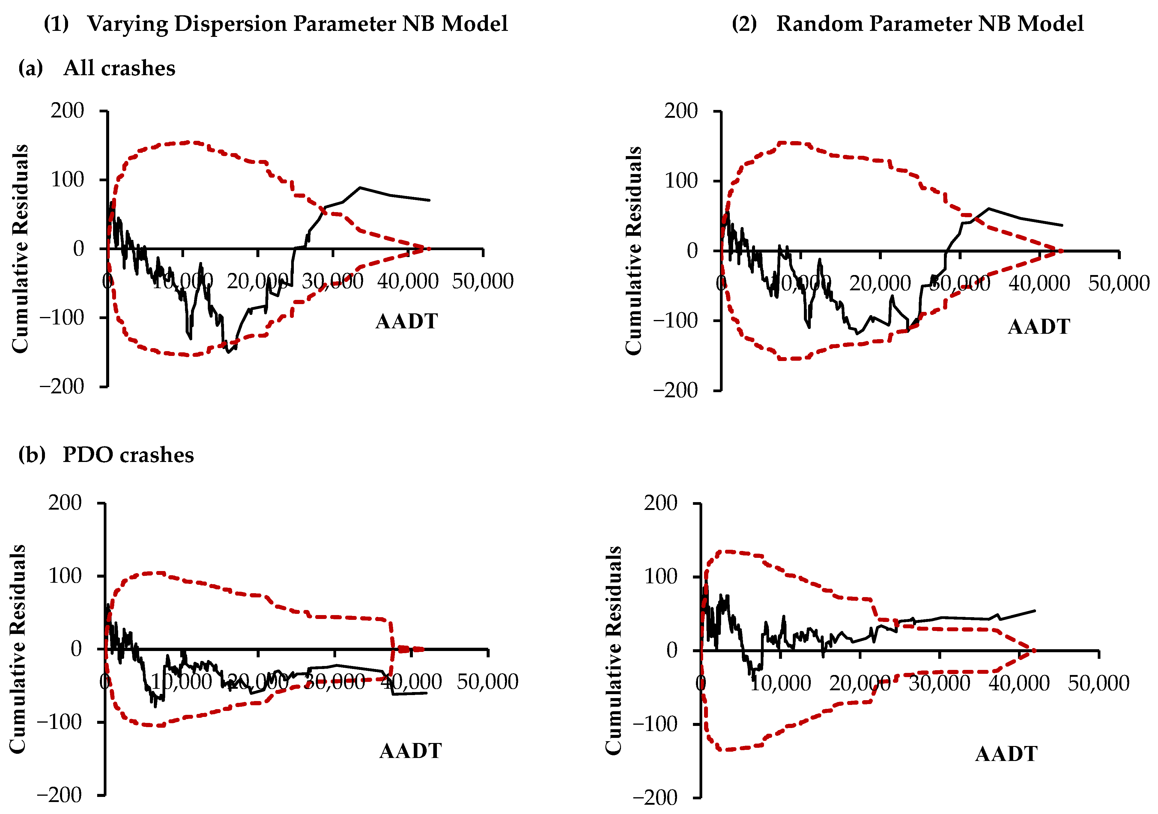
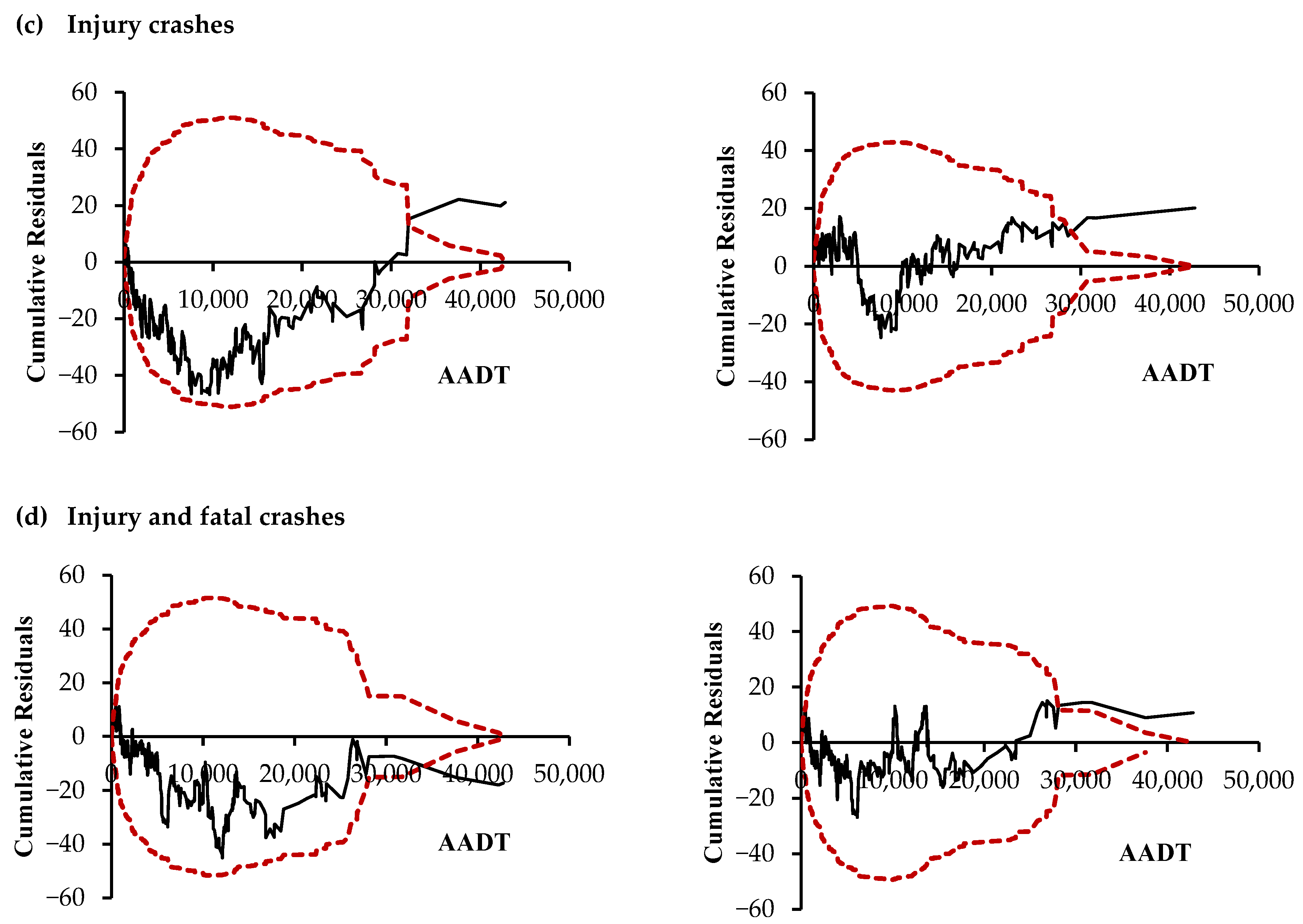
4.1. Crash Prediction Models

Table 2 provides the coefficient estimates of the two derivatives of NB models, that is, the varying dispersion parameter negative binomial model (VDPNB) and random parameter negative binomial model (RPNB) for different crash severity levels. The confidence level for retaining variables in the model was 95%. Following Tang et al. [37], the random parameters were determined through 200 Halton draws.
Both models produced coefficient estimates that indicate plausible signs and direction. For instance, the coefficient estimates of the significant variables are similar in the two different regression models for each crash severity level. However, the magnitude of the estimated coefficients for predictor variables varies across different severity levels. This observation supports estimating separate models for different severity levels, acknowledging potential differences in crash-contributing factors across these levels.
Traffic volume, segment length, lane width, number of lanes, and parking types were significant variables in both models for all crashes and PDO crashes. For injury crashes and injury and fatal crashes, all variables were significant in the VDPNB model except the number of lanes. Moreover, in the RPNB model, the standard deviations of two parameters (traffic volume and lane width) significantly differed from zero. Thus, they were estimated as random parameters.
The crash frequency is positively associated with the traffic variable and segment length for all crash severity levels in the developed models, meaning that an increased traffic volume will result in a higher expected crash frequency. However, it is noteworthy that the resulting increase in expected crash frequency is not uniform across severity levels. The variable ‘number of lanes’ shows an interesting association with the crash frequency. It has a significant negative relationship with all crashes and PDO crashes, but it is an insignificant predictor of injury crashes and injury and fatal crashes. The lane width shows a significant negative association with crash frequency for all severity levels and both model types. The negative impact is the highest for PDO crashes. Parking type is a significant predictor for all crashes and PDO crashes. However, for injury crashes and injury and fatal crashes, only one parking type (i.e., parallel parking) is significant.
Table 2 also provides the results for the overdispersion parameter estimated as a function of various predictor variables in the VDPNB models. It shows that the segment length positively correlates with dispersion in all models. At the same time, traffic volume negatively affects the dispersion parameter, similar to Khodadadi et al. [43]. The number of lanes is another significant predictor of the dispersion in the data, only for all and PDO crashes. The nature of the relationship is positive. The number of lanes is insignificant for injury and injury and fatal crashes. The lane width is not associated with dispersion in any model. Parking type and dispersion in the data have a significant negative association for all models except the PDO crash model’s perpendicular, angled, and mixed parking variables.
Before comparing the hotspot identification performance, the developed models were examined for the goodness of fit via log-likelihood, AIC, and cumulative residual (CURE) plots. The smaller the log-likelihood and AIC values, the better the model performance. The CURE plots are tools used to assess the performance of different models visually and objectively. According to Hauer [15], when residual plots closely oscillate around the zero line, it indicates a better model fit to the data. Moreover, the CURE plots for unbiased SPF typically fall within the boundaries of two standard deviations.
The CURE plots indicated that RPNB models outperformed VDPNB models across all severity levels as the obtained estimates oscillated closely to the zero line for RPNB models. These results are consistent with findings from the likelihood and AIC values. In addition, most estimates were clustered on the left side, which was anticipated due to the low traffic volume of many road segments. In general, the CURE plots remained within two standard deviations for most AADT values except for the extreme right ends of the plots. Figure 1 presents the CURE plots for VDPNB and RPNB models by crash severity.

4.2. Hotspot Identification Comparison

Table 3, Table 4 and Table 5 show the results for HCCT, CSCT, and ARDT, respectively, which compare the HSID performance of the EB and PSI estimates for VDPNB and RPNB models for total, PDO, injury, and injury and fatal crashes. To find hotspots, the road segments were ranked by the level of risk (i.e., EB estimate and PSI measure) they were characterised by, and those with the highest risk were considered hotspots. The current study assessed the HSID performance for the top 2.5%, 5.0%, 7.5%, and 10.0% sites. The higher the values for HCCT and CSCT scores and the lower the values for ARDT, the better the HSID performance of the given method.
Guo et al. [31] advised to divide the data into at least two subperiods for more accurate evaluation. This allows us to check whether the performance of the given HSID method changes between the initial and the subsequent periods. However, Guo et al. [31] further noticed that the aggregation of crash data into only two subperiods may only be suboptimal in terms of the accuracy of the performance evaluation of HSID methods. Therefore, analysts should consider more than two subperiods. This study computes the HSID performance comparison criteria scores for more than two subperiods. Therefore, we divided six-year crash data into three different subperiods, each with two years (i.e., P1: 2010–11, P2: 2012–13, P3: 2014–15). In addition, test scores were computed for two different setups to confirm the robustness of the results, with one setup using P1 as the first period and P2 and P3 as the subsequent periods. Another setup used P2 as the initial period and P3 as the subsequent period. Please refer to Guo et al. (2020) for more information about subperiods [31].
It is shown in Table 3 that from the point of view of the HCCT, the best-performing method of the two (i.e., EB and PSI) was the EB estimates for both RPNB and VDPNB models in ranking the top 2.5%, 5.0%, 7.5%, and 10.0% hazardous sites. Moreover, RPNB models outperformed the VDPNB models when HCCT evaluated the EB estimates for these two modelling frameworks. These results apply to both setups (i.e., (a. (P1 *, P2, P3) and b. (P2 *, P3)), where a period with the asterisk denotes the initial period in each target setting). For example, for all crashes, the EB method for RPNB models provides the highest scores for the HCCT in identifying hotspots compared to the EB estimates of the VDPNB model. The results for PDO, injury, and injury and fatal crashes also confirmed that EB estimates for the RPNB model provide better hotspot identification performance than other estimates. Among the two modelling frameworks (i.e., VDPNB and RPNB) and HSID methods (i.e., EB and PSI), the PSI estimates for VDPNB models resulted in low scores on HCCT, indicating the worst performance.
Similarly, the scores on the CSCT showed that EB estimates perform better than the corresponding PSI estimates in identifying the top 2.5%, 5.0%, 7.5%, and 10.0% of hotspots for both RPNB and VDPNB models (Table 4). Comparing the EB estimates for VDPNB and RPNB models, the scores of the CSCT favoured the RPNB model for all crash severity levels. Among the two modelling frameworks (i.e., VDPNB and RPNB) and HSID methods (i.e., EB and PSI), the PSI estimates for VDPNB models resulted in low scores on CSCT, indicating the worst performance.
Table 5 illustrates the performance analysis based on ARDT. Like the HCCT and CSCT, the EB method outperformed the PSI method on ARDT in both comparison periods. However, the comparison of the performance of the EB method for VDPNB and RPNB models revealed that the former performed better than the latter (i.e., lowest values of the EB method have resulted for VDPNB model in both setups (i.e., (a. (P1 *, P2, P3) and b. (P2 *, P3)) for the top 2.5%, 5.0%, 7.5%, and 10.0% of hotspots). Among the two modelling frameworks (i.e., VDPNB and RPNB) and HSID methods (i.e., EB and PSI), the PSI estimates for VDPNB resulted in extremely high scores on ARDT in most cases, indicating the worst performance.
To summarise, with only a few exceptions to the general trend, it could be safely concluded that the EB method outperforms the PSI in the HSID for all crash severity levels studied in this paper.

5. Discussion

Identification of crash hotspots based on statistical modelling-based approaches, such as the EB or PSI methods, requires analysts to choose the model specification that best handles the heterogeneity associated with the crash data. While the traditional NB model can effectively approximate the underlying crash occurrences, it has certain limitations [17]. Therefore, more flexible models are recommended since overdispersion in crash data can arise from various sources and is unknown to analysts. The above results evaluate the hotspot identification performance of the EB and PSI estimates obtained for the VDPNB and RPNB models. However, we briefly discuss the modelling results before discussing HSID results, following Lord and Park [44], who indicated that it is vital for transportation safety analysts to understand the structure of the mean function. Thus, the first part of this section discusses the relationship between covariates and crash frequency. The second part is more focused on discussing the HSID performance of the EB and PSI methods for the VDPNB model with the RPNB model.
The data modelling revealed a positive association between crash frequency and exposure variables (i.e., traffic volume and segment length). This was not surprising as an increase in the number of vehicles on roadways increases the risk of conflicts, which are converted into actual collisions in a few instances. With the unchanging design and monotonous traffic conditions, drivers tend to speed more on longer homogenous segments. Given the acknowledged association between speed and the risk of crash involvement [56], this might lead to more collisions when the segments are long. The coefficients of traffic volume in injury and injury and fatal crash models were higher than those in PDO and all crash models. This is somewhat counterintuitive and needs further explanation. Antwerp is in Flanders, a Belgian region with the highest proportion of people who commute to work by bike (around 17%). Antwerp is also one of the region’s most bike-friendly cities, with a large proportion of people (around 29%) who use bikes to commute [57]. The higher the proportion of cyclists in traffic, the higher the exposure to crash risk and, thus, the higher the number of crashes involving cyclists. It has been a fact that vulnerable road users, including cyclists, are more involved in severe injury crashes than motorists. For instance, only in the European Union do vulnerable road users form about 46% of all traffic fatalities and 53% of all seriously injured crash victims [58]. Thus, the higher presence of cyclists in traffic could result in more severe injury crashes. This effect was captured by higher coefficients for traffic volume in the estimated injury and injury and fatal crash models.
The lane width was found to have a significant adverse effect on the crash frequency, indicating improved road safety due to wider lanes. Mohammed [59] attempted to explain this association and argued that it makes sense to assume that wider lanes improve safety because they provide an additional space and time threshold that allows drivers to take corrective actions and avoid collision compared to narrower lanes.
The number of lanes was a significant predictor of crash frequency only in all crash and PDO crash models. The nature of the association was negative, meaning a decrease in crash frequency as the number of lanes increased. This finding surprised us since it contradicts other studies, for instance, Noland and Oh [60]. A potential reason could be that an additional lane decreases the traffic density on the roadways, contributing to more safety, particularly for PDO crashes. Also, an additional lane(s), similar to a wider lane, provides the driver extra space and time to take corrective action.
Parking type (including parallel, perpendicular, angle, and mixed parking) was a significant predictor of crash frequency in all and PDO crash models. However, only parallel parking was significant in the case of injury crashes and injury and fatal crash models, while other parking types were insignificant. It was observed that the association was not uniform across different parking types and models. All and PDO crashes increased more for other types of parking than parallel parking. In contrast, injury and injury and fatal crashes were more prevalent in the case of parallel parking. This could be explained by the fact that when drivers encounter complex parking designs, e.g., perpendicular, angle, or mixed, they drive cautiously and relatively slower, which helps them avoid severe crashes. However, this cautious behaviour appeared less effective in avoiding the PDO crashes and, subsequently, all crashes. In addition, perpendicular and angle parking provide greater separation (buffer zone) between the vehicles and vulnerable road users compared to parallel parking or no parking, which could be another reason for less severe crashes in the case of perpendicular, angle, or mixed parking settings and more injury crashes in case of parallel parking. These results can interest policymakers because higher injury severity crashes often lead to higher social costs [56], and minimizing those crashes will have economic advantages to society and help improve the sustainability of the transportation system.
The developed VDPNB models provided crucial information about the sources of the overdispersion in the data. Characterizing the dispersion parameter as a function of the covariates helped account for the extra variation in the data. The results suggested that all predictor variables except the lane width influence the overdispersion parameter. This was a preconceived outcome as the descriptive analysis (Table 1) provided clues about overdispersion in the data. For instance, there was an abundance of shorter homogenous segments in the data, probably because of the urban context and the studied road class, i.e., the accessibility objective of the local roads. According to Cafiso et al. [42], dispersion parameter variation matters more in shorter segments than in longer ones. In another instance, a little over 1550 of 2467 segments in the dataset had parallel parking, while only 164 had other parking categories. The excessive presence of parallel parking in the study area may have significantly contributed to this overdispersion. Similar trends were also observed for the number of lanes.
The estimated models were used to compute the EB estimates and PSI, which were tested for the HSID performance using three generalised criteria (i.e., HCCT, CSCT, and ARDT). The CSCT measured how well the methods could consistently identify sites with poor safety performance over time. The HCCT evaluated the methods for the number of the same hotspots identified in subsequent periods. These tests established that the EB estimates for the RPNB model (except for ARDT) outperformed the PSI estimates for the RPNB and VDPNB models and the corresponding EB estimates for the VDPNB model. A solid theoretical basis supports this because the EB method takes advantage of the observed and predicted values in its statistics, which in turn increases the reliability of its results and thus improves the precision of safety estimation. Moreover, the EB method also corrects for regression to the mean bias. All these characteristics of the EB method for estimating the safety of the highway network sites allow for the identification of the relative contributions of random variation, general factors, and local factors to the observed number of crashes. In practice, the EB method proved its efficiency in the current and other studies [10,12,19,22]. The PSI methods, on the other hand, seem to be reasonably inconsistent in most cases as opposed to the findings by Li and Wang [19]. The PSI method is primarily affected by the predicted value and, consequently, the validity of the developed crash prediction model. As crashes’ predicted value increases, a site’s likelihood of being selected as a hotspot increases.
This study has some limitations. For example, while interpreting those results, it should be noted that the current study did not explore its different possible parametrisation or functional forms while estimating the dispersion parameter as a function of different variables in the VDPNB models. Thus, we could not comment on the most appropriate parametrisation of the dispersion parameter for the current data and, hence, the consequent HSID results. Nevertheless, the results for the HSID favoured the EB estimates compared to the PSI in general, thereby confirming the findings of many past studies. In this study, different levels of severity were investigated (i.e., all, PDO, injury, and injury and fatal). However, different crash types (e.g., angle, head-on, rear-end, and sideswipe) could be considered in future studies. Furthermore, future studies could reproduce this type of analysis for other road facilities (e.g., intersections) and other road types (e.g., rural roads or expressways). The findings of this study are based on the analysis of actual data. Without an a priori knowledge of which sites are truly hazardous and which are relatively safe, detecting false positives (i.e., erroneous selection of relatively safe sites as hotspots) becomes problematic. Future research could focus on achieving more conclusive outcomes by simulating collision data that establish which sites are hazardous in advance, allowing for an assessment of whether the proposed method can accurately identify these hazardous locations.

6. Conclusions

The principal aim of this paper was to evaluate the performance of two HSID methods (i.e., EB and PSI) using the estimates obtained from two different variants of the NB model (i.e., VDPNB and RPNB). The VDPNB models allow the dispersion parameter to vary across observations, while in the RPNB model, the coefficient estimates of each parameter can vary across observations. Predictive models were developed for all crashes, PDO crashes, injury crashes, and injury and fatal crashes. The explanatory variables included the length of homogenous road segments, the traffic volume, the lane width, the number of lanes, and the on-street parking type. The findings revealed significant associations between crash frequency and site characteristics in both models. Moreover, the results also identified an association between the dispersion parameter and site characteristics in the VDPNB models. The VDPNB and RPNB model results were used in computing EB estimates and PSI measures for HSID.
Three generalised criteria were used to evaluate the performance of the HSID methods (i.e., EB estimates and PSI measures) obtained from the VDPNB and RPNB models. These HSID performance criteria indicated stable, consistent, and robust results in identifying the top 2.5%, 5.0%, 7.5%, and 10.0% of the hazardous sites utilizing the EB estimates of the VDPNB and RPNB models compared to the PSI method. When the EB estimates were compared for two variants of the NB model, the RPNB model outperformed the VDPNB model in most cases. The reliable HSID method accurately detects the potential crash-prone sites and consequently makes sure to use public funds related to road safety efficiently. This ultimately leads to safer roads and improved overall safety. Additionally, inaccurately identifying crash hotspots can lead to inefficient allocation of limited resources, putting the effectiveness of sustainable safety interventions at risk.

Author Contributions

Conceptualisation, M.W.K., A.P., P.D.W. and H.D.B.; methodology, M.W.K., A.P., H.D.B., P.D.W. and T.B.; software, M.W.K.; formal analysis, M.W.K.; investigation, M.W.K.; resources, A.P., P.D.W., H.D.B. and T.B.; data curation, M.W.K.; writing—original draft preparation, M.W.K.; writing—review and editing, A.P. and H.D.B.; supervision, A.P., H.D.B., T.B. and P.D.W. All authors have read and agreed to the published version of the manuscript.

Funding

This research received no external funding.

Institutional Review Board Statement

Not applicable.

Informed Consent Statement

Not applicable.

Data Availability Statement

The data presented in this study are unavailable because of data ownership and copyrights.

Acknowledgments

The authors thank Antwerp Police for providing crash data for this work, Lantis (a mobility company of Antwerp city) for providing the necessary traffic data, and the Flemish Government for providing the road infrastructure data.

Conflicts of Interest

The authors declare no conflicts of interest.

References

  1. Haddak, M.M.; Lefèvre, M.; Havet, N. Willingness-to-Pay for Road Safety Improvement. Transp. Res. Part Policy Pract. 2016, 87, 1–10. [Google Scholar] [CrossRef]
  2. Corben, B.; Peiris, S.; Mishra, S. The Importance of Adopting a Safe System Approach—Translation of Principles into Practical Solutions. Sustainability 2022, 14, 2559. [Google Scholar] [CrossRef]
  3. United Nations. Improving Global Road Safety; United Nations: New York, NY, USA, 2020. [Google Scholar]
  4. United Nations. The UN Sustainable Development Goals; United Nations: New York, NY, USA, 2016. [Google Scholar]
  5. European Commission EU Strategic Action Plan on Road Safety; European Commission: Brussels, Belgium, 2018.
  6. European Commission. EU Road Safety Policy Framework 2021–2030—Next Steps towards Vision Zero; European Commission: Brussels, Belgium, 2019. [Google Scholar]
  7. Highway Safety Manual (HSM); AASHTO, American Association of State and Highway Transportation Officials: Washington DC, USA, 2010; ISBN 978-1-56051-477-0.
  8. Road Safety Manual; Technical Committee on Road Safety C13; World Road Association: London, UK, 2019.
  9. Global Status Report on Road Safety 2023; World Health Organization: Geneva, Switzerland, 2023; ISBN 92-4-156506-3.
  10. Montella, A. A Comparative Analysis of Hotspot Identification Methods. Accid. Anal. Prev. 2010, 42, 571–581. [Google Scholar] [CrossRef] [PubMed]
  11. Elvik, R. A Survey of Operational Definitions of Hazardous Road Locations in Some European Countries. Accid. Anal. Prev. 2008, 40, 1830–1835. [Google Scholar] [CrossRef] [PubMed]
  12. Cheng, W.; Washington, S.P. Experimental Evaluation of Hotspot Identification Methods. Accid. Anal. Prev. 2005, 37, 870–881. [Google Scholar] [CrossRef]
  13. Laughland, J.C.; Haefner, L.E.; Hall, J.W.; Clough, D.R. Methods for Evaluating Highway Safety Improvements; Transportation Research Board: Washington, DC, USA, 1975. [Google Scholar]
  14. Hauer, E.; Persaud, B.N. Problem of Identifying Hazardous Locations Using Accident Data. Transp. Res. Rec. 1984, 975, 36–43. [Google Scholar]
  15. Hauer, E. Observational before/after Studies in Road Safety. Estimating the Effect of Highway and Traffic Engineering Measures on Road Safety; Elsevier Science Inc.: Tarrytown, NY, USA, 1997; ISBN 978-0-08-043053-9. [Google Scholar]
  16. Cheng, W.; Washington, S. New Criteria for Evaluating Methods of Identifying Hot Spots. Transp. Res. Rec. 2008, 2083, 76–85. [Google Scholar] [CrossRef]
  17. Lord, D.; Mannering, F. The Statistical Analysis of Crash-Frequency Data: A Review and Assessment of Methodological Alternatives. Transp. Res. Part Policy Pract. 2010, 44, 291–305. [Google Scholar] [CrossRef]
  18. Wang, K.; Zhao, S.; Ivan, J.N.; Ahmed, I.; Jackson, E. Evaluation of Hot Spot Identification Methods for Municipal Roads. J. Transp. Saf. Secur. 2020, 12, 463–481. [Google Scholar] [CrossRef]
  19. Li, J.; Wang, X. Hotspot Identification on Urban Arterials at the Meso Level. Accid. Anal. Prev. 2022, 169, 106632. [Google Scholar] [CrossRef]
  20. Wan, Y.; He, W.; Zhou, J. Urban Road Accident Black Spot Identification and Classification Approach: A Novel Grey Verhuls–Empirical Bayesian Combination Method. Sustainability 2021, 13, 11198. [Google Scholar] [CrossRef]
  21. Meng, Y.; Wu, L.; Ma, C.; Guo, X.; Wang, X. (Bruce) A Comparative Analysis of Intersection Hotspot Identification: Fixed vs. Varying Dispersion Parameters in Negative Binomial Models. J. Transp. Saf. Secur. 2020, 14, 305–322. [Google Scholar] [CrossRef]
  22. Manepalli, U.R.R.; Bham, G.H. An Evaluation of Performance Measures for Hotspot Identification. J. Transp. Saf. Secur. 2016, 8, 327–345. [Google Scholar] [CrossRef]
  23. Zou, Y.; Lord, D.; Zhang, Y.; Peng, Y. Comparison of Sichel and Negative Binomial Models in Estimating Empirical Bayes Estimates. Transp. Res. Rec. 2013, 2392, 11–21. [Google Scholar] [CrossRef]
  24. Kononov, J.; Durso, C.; Lyon, C.; Allery, B. Level of Service of Safety Revisited. Transp. Res. Rec. 2015, 2514, 10–20. [Google Scholar] [CrossRef]
  25. Cafiso, S.; Di Silvestro, G. Performance of Safety Indicators in Identification of Black Spots on Two-Lane Rural Roads. Transp. Res. Rec. 2011, 2237, 78–87. [Google Scholar] [CrossRef]
  26. Washington, S.; Haque, M.M.; Oh, J.; Lee, D. Applying Quantile Regression for Modeling Equivalent Property Damage Only Crashes to Identify Accident Blackspots. Accid. Anal. Prev. 2014, 66, 136–146. [Google Scholar] [CrossRef]
  27. Karamanlis, I.; Nikiforiadis, A.; Botzoris, G.; Kokkalis, A.; Basbas, S. Towards Sustainable Transportation: The Role of Black Spot Analysis in Improving Road Safety. Sustainability 2023, 15, 14478. [Google Scholar] [CrossRef]
  28. Maher, M.J.; Mountain, L.J. The Identification of Accident Blackspots: A Comparison of Current Methods. Accid. Anal. Prev. 1988, 20, 143–151. [Google Scholar] [CrossRef]
  29. Khodadadi, A.; Tsapakis, I.; Shirazi, M.; Das, S.; Lord, D. Derivation of the Empirical Bayesian Method for the Negative Binomial-Lindley Generalized Linear Model with Application in Traffic Safety. Accid. Anal. Prev. 2022, 170, 106638. [Google Scholar] [CrossRef]
  30. Huang, H.; Chin, H.C.; Haque, M.M. Hotspot Identification: A Full Bayesian Hierarchical Modeling Approach. In Transportation and Traffic Theory 2009: Golden Jubilee: Papers Selected for Presentation at ISTTT18, a Peer Reviewed Series Since 1959; Lam, W.H.K., Wong, S.C., Lo, H.K., Eds.; Springer: Boston, MA, USA, 2009; pp. 441–462. ISBN 978-1-4419-0820-9. [Google Scholar]
  31. Guo, X.; Wu, L.; Lord, D. Generalized Criteria for Evaluating Hotspot Identification Methods. Accid. Anal. Prev. 2020, 145, 105684. [Google Scholar] [CrossRef] [PubMed]
  32. Mendes, O.B.B.; Larocca, A.P.C.; Rodrigues Silva, K.; Pirdavani, A. Assessing the Performance of Highway Safety Manual (HSM) Predictive Models for Brazilian Multilane Highways. Sustainability 2023, 15, 10474. [Google Scholar] [CrossRef]
  33. Zou, Y.; Ash, J.E.; Park, B.-J.; Lord, D.; Wu, L. Empirical Bayes Estimates of Finite Mixture of Negative Binomial Regression Models and Its Application to Highway Safety. J. Appl. Stat. 2018, 45, 1652–1669. [Google Scholar] [CrossRef]
  34. Champahom, T.; Jomnonkwao, S.; Banyong, C.; Nambulee, W.; Karoonsoontawong, A.; Ratanavaraha, V. Analysis of Crash Frequency and Crash Severity in Thailand: Hierarchical Structure Models Approach. Sustainability 2021, 13, 10086. [Google Scholar] [CrossRef]
  35. Khattak, M.W.; Pirdavani, A.; De Winne, P.; Brijs, T.; De Backer, H. Estimation of Safety Performance Functions for Urban Intersections Using Various Functional Forms of the Negative Binomial Regression Model and a Generalized Poisson Regression Model. Accid. Anal. Prev. 2021, 151, 105964. [Google Scholar] [CrossRef] [PubMed]
  36. Mićić, S.; Vujadinović, R.; Amidžić, G.; Damjanović, M.; Matović, B. Accident Frequency Prediction Model for Flat Rural Roads in Serbia. Sustainability 2022, 14, 7704. [Google Scholar] [CrossRef]
  37. Tang, H.; Gayah, V.V.; Donnell, E.T. Evaluating the Predictive Power of an SPF for Two-Lane Rural Roads with Random Parameters on out-of-Sample Observations. Accid. Anal. Prev. 2019, 132, 105275. [Google Scholar] [CrossRef] [PubMed]
  38. Intini, P.; Berloco, N.; Coropulis, S.; Gentile, R.; Ranieri, V. The Use of Macro-Level Safety Performance Functions for Province-Wide Road Safety Management. Sustainability 2022, 14, 9245. [Google Scholar] [CrossRef]
  39. Montella, A.; Marzano, V.; Mauriello, F.; Vitillo, R.; Fasanelli, R.; Pernetti, M.; Galante, F. Development of Macro-Level Safety Performance Functions in the City of Naples. Sustainability 2019, 11, 1871. [Google Scholar] [CrossRef]
  40. Pirdavani, A.; Brijs, T.; Bellemans, T.; Kochan, B.; Wets, G. Application of Different Exposure Measures in Development of Planning-Level Zonal Crash Prediction Models. Transp. Res. Rec. 2012, 2280, 145–153. [Google Scholar] [CrossRef]
  41. Hauer, E. Overdispersion in Modelling Accidents on Road Sections and in Empirical Bayes Estimation. Accid. Anal. Prev. 2001, 33, 799–808. [Google Scholar] [CrossRef]
  42. Cafiso, S.; Di Silvestro, G.; Persaud, B.; Begum, M.A. Revisiting Variability of Dispersion Parameter of Safety Performance for Two-Lane Rural Roads. Transp. Res. Rec. 2010, 2148, 38–46. [Google Scholar] [CrossRef]
  43. Khodadadi, A.; Tsapakis, I.; Das, S.; Lord, D.; Li, Y. Application of Different Negative Binomial Parameterizations to Develop Safety Performance Functions for Non-Federal Aid System Roads. Accid. Anal. Prev. 2021, 156, 106103. [Google Scholar] [CrossRef] [PubMed]
  44. Lord, D.; Park, P.Y.-J. Investigating the Effects of the Fixed and Varying Dispersion Parameters of Poisson-Gamma Models on Empirical Bayes Estimates. Accid. Anal. Prev. 2008, 40, 1441–1457. [Google Scholar] [CrossRef] [PubMed]
  45. Anastasopoulos, P.C.; Mannering, F.L. A Note on Modeling Vehicle Accident Frequencies with Random-Parameters Count Models. Accid. Anal. Prev. 2009, 41, 153–159. [Google Scholar] [CrossRef] [PubMed]
  46. Lord, D.; Persaud, B.N. Accident Prediction Models With and Without Trend: Application of the Generalized Estimating Equations Procedure. Transp. Res. Rec. 2000, 1717, 102–108. [Google Scholar] [CrossRef]
  47. Shankar, V.N.; Albin, R.B.; Milton, J.C.; Mannering, F.L. Evaluating Median Crossover Likelihoods with Clustered Accident Counts: An Empirical Inquiry Using the Random Effects Negative Binomial Model. Transp. Res. Rec. 1998, 1635, 44–48. [Google Scholar] [CrossRef]
  48. Mitra, S.; Washington, S. On the Nature of Over-Dispersion in Motor Vehicle Crash Prediction Models. Accid. Anal. Prev. 2007, 39, 459–468. [Google Scholar] [CrossRef] [PubMed]
  49. Hou, Q.; Huo, X.; Tarko, A.P.; Leng, J. Comparative Analysis of Alternative Random Parameters Count Data Models in Highway Safety. Anal. Methods Accid. Res. 2021, 30, 100158. [Google Scholar] [CrossRef]
  50. Greene, W.H. Econometric Analysis, 4th ed.; Prentice Hall: Englewood Cliffs, NJ, USA, 2007; pp. 201–215. [Google Scholar]
  51. Bhat, C.R. Simulation Estimation of Mixed Discrete Choice Models Using Randomized and Scrambled Halton Sequences. Transp. Res. Part B Methodol. 2003, 37, 837–855. [Google Scholar] [CrossRef]
  52. Xu, P.; Zhou, H.; Wong, S.C. On Random-Parameter Count Models for out-of-Sample Crash Prediction: Accounting for the Variances of Random-Parameter Distributions. Accid. Anal. Prev. 2021, 159, 106237. [Google Scholar] [CrossRef] [PubMed]
  53. Persaud, B.; Lyon, C.; Nguyen, T. Empirical Bayes Procedure for Ranking Sites for Safety Investigation by Potential for Safety Improvement. Transp. Res. Rec. 1999, 1665, 7–12. [Google Scholar] [CrossRef]
  54. Hauer, E. Lane Width and Safety. Literature. 2000. Available online: https://www.academia.edu/21401042/Lane_width_and_safety_Literature (accessed on 11 December 2023).
  55. Pirdavani, A.; Bellemans, T.; Brijs, T.; Wets, G. Application of Geographically Weighted Regression Technique in Spatial Analysis of Fatal and Injury Crashes. J. Transp. Eng. 2014, 140, 04014032. [Google Scholar] [CrossRef]
  56. Brijs, T.; Pirdavani, A. Urban and Suburban Arterials. In Safe Mobility: Challenges, Methodology and Solutions; Lord, D., Washington, S., Eds.; Transport and Sustainability; Emerald Publishing Limited: Bingley, UK, 2018; Volume 11, pp. 85–106. ISBN 978-1-78635-223-1. [Google Scholar]
  57. Swennen, B. Antwerp’s Cycling Policy Plan 2015–2019—A Lot of Ambition and a Good Plan! Available online: https://www.ecf.com/news-and-events/news/antwerps-cycling-policy-plan-2015-2019-lot-ambition-and-good-plan (accessed on 16 November 2022).
  58. Olszewski, P.; Szagała, P.; Rabczenko, D.; Zielińska, A. Investigating Safety of Vulnerable Road Users in Selected EU Countries. J. Saf. Res. 2019, 68, 49–57. [Google Scholar] [CrossRef]
  59. Mohammed, H. The Influence of Road Geometric Design Elements on Highway Safety. Int. J. Civ. Eng. Technol. 2013, 4, 146–162. [Google Scholar]
  60. Noland, R.B.; Oh, L. The Effect of Infrastructure and Demographic Change on Traffic-Related Fatalities and Crashes: A Case Study of Illinois County-Level Data. Accid. Anal. Prev. 2004, 36, 525–532. [Google Scholar] [CrossRef] [PubMed]
Figure 1. Cumulative residual (CURE) plots for VDPNB and RPNB models.
Sustainability 16 01537 g001aSustainability 16 01537 g001b
Table 1. Descriptive statistics of the dataset for the urban roads of Antwerp.
Traffic and Road Segment Variables
VariablesMinimumMaximumMeanStd. Dev.
AADT (veh/day)2242,78348426543
Segment length (km)0.061.5570.1090.104
Lane width (m)2.505.003.510.50
No. of Lanes 11 = 749, 2 = 1054, 3 = 664
Parking Type 20 = 738 sites, 1 = 1565 sites, 2 = 164 sites
Parking Arrangement 30 = 740 sites, 1 = 719 sites, 2 = 949 sites, 3 = 59 sites
Crash Frequency
MinimumMaximumMeanStd. Dev.
All crashes 4 (six years: 2010–2015)0907.5210.28
(P1: 2010–2011)0282.383.078
(P2: 2012–2013)0332.583.290
(P3: 2014–2015)0192.162.761
Fatal and injury crashes (six years: 2010–2015)0442.014.421
(P1: 2010–2011)0120.581.222
(P2: 2012–2013)0140.661.302
(P3: 2014–2015)0100.571.132
Injury crashes (six years: 2010–2015)0431.994.402
(P1: 2010–2011)0120.651.339
(P2: 2012–2013)0110.701.344
(P3: 2014–2015)0100.651.177
PDO crashes (six years: 2010–2015)0675.516.937
(P1: 2010–2011)0201.852.499
(P2: 2012–2013)0221.992.577
(P3: 2014–2015)0151.652.099
1 1 = one lane, 2 = two lanes, 3 = three or more lanes; 2 0 = no parking, 1 = parallel parking, 2 = others (perpendicular, angled, and mixed parking); 3 0 = no parking, 1 = one-sided parking, 2 = two-sided parking, 3 = others (three-sided and four-sided parking in case of divided roads); 4 = six-year crash data divided into three subperiods indicating different data aggregations for assessing the HSID performance.
Table 2. Estimated coefficients for the varying dispersion parameter negative binomial (VDPNB) and random parameter negative binomial (RPNB) models.
All
Crashes
PDO
Crashes
Injury
Crashes
Injury and
Fatal Crashes
Coef. 1
(Std. Err.)
Coef.
(Std. Err.)
Coef.
(Std. Err.)
Coef.
(Std. Err.)
(a). VDPNB
Intercept1.513 ***
(0.251)
1.940 ***
(0.250)
−1.883 ***
(0.405)
−1.814 ***
(0.394)
Seg. Length0.641 ***
(0.034)
0.673 ***
(0.018)
0.585 ***
(0.050)
0.608 ***
(0.049)
Traffic Vol.0.293 ***
(0.018)
0.246 ***
(0.034)
0.522 ***
(0.029)
0.538 ***
(0.029)
No. of Lanes
Two lanes vs. one lane−0.260 ***
(0.061)
−0.361 ***
(0.061)
--
Three or more lanes vs. one lane−0.166 **
(0.083)
−0.343 ***
(0.085)
--
Lane width−0.125 ***
0.047
−0.204 ***
0.049
−0.145 *
(0.075)
−0.156 **
(0.074)
Parking Type
Parallel parking vs. no parking0.371 ***
(0.055)
0.476 ***
(0.056)
0.127 *
(0.072)
0.084 **
(0.073)
Other parking types 2 vs. no parking0.549 **
(0.095)
0.796 ***
(0.101)
0.013
(0.130)
0.070
(0.120)
Dispersion parameter
Intercept0.397
(0.584)
0.116
(0.622)
2.096 **
0.991
2.202 **
(0.973)
Seg. Length0.140 **
(0.070)
0.324 ***
(0.075)
0.254 **
(0.111)
0.239 **
(0.108)
AADT−0.180 ***
(0.040)
−0.094 **
(0.043)
−0.265 ***
(0.071)
−0.347 ***
(0.067)
No. of Lanes
Two lanes vs. one lane0.511 ***
(0.154)
0.511 ***
(0.166)
--
Three or more lanes vs. one lane0.892 ***
(0.188)
0.847 ***
(0.201)
--
Parking Type
Parallel parking vs. no parking−0.546 ***
(0.111)
−0.601 ***
(0.119)
−0.679 ***
(0.154)
−0.718 ***
(0.155)
Other parking types vs. no parking−0.359 *
(0.188)
−0.218 *
(0.194)
−0.938 **
(0.381)
−1.302 **
(0.418)
Log-likelihood −5373.247 −4918.777 −3031.631 −3047.820
AIC10,770.5009861.6006087.3006119.600
(b). RPNB Model
Intercept1.463 ***
(0.228)
1.637 ***
(0.231)
−2.159 ***
(0.346)
−2.156 ***
(0.349)
SD of intercept0.194 *
(0.018)
0.017 *
(0.018)
0.022 *
(0.026)
0.064 **
(0.026)
Seg. Length0.656 ***
(0.026)
0.657 ***
(0.027)
0.529 ***
(0.040)
0.522 ***
(0.040)
AADT0.300 ***
(0.015)
0.241 ***
(0.016)
0.553 ***
(0.025)
0.549 ***
(0.025)
SD of AADT0.027 ***
(0.002)
0.046 ***
(0.002)
0.009 ***
(0.003)
0.010 ***
(0.003)
No. of Lanes
Two lanes vs. one lane−0.317 ***
(0.062)
−0.399 ***
(0.062)
--
Three or more lanes vs. one lane−0.283 **
(0.075)
−0.369 ***
(0.077)
--
Lane width−0.205 ***
(0.047)
−0.221 ***
(0.047)
−0.211 ***
(0.071)
−0.200 ***
(0.072)
SD of lane width0.014 ***
(0.005)
0.019 ***
(0.005)
0.123 ***
(0.007)
0.114 ***
(0.007)
Parking Type
Parallel parking vs. no parking0.472 ***
(0.045)
0.611 **
(0.046)
0.181 ***
(0.061)
0.162 ***
(0.062)
Other parking types vs. no parking0.623 **
(0.077)
0.842 ***
(0.078)
--
Dispersion parameter2.233 ***
(0.102)
2.361 ***
(0.121)
2.054 **
(0.171)
1.953 **
(0.158)
Log-likelihood−5216.016−4738.422−2958.796−2987.567
AIC10,464.0309508.8445949.5916007.135
The estimates’ means and standard errors (in parentheses) are used to sum up the results.; 1 ***: p < 0.01, **: p < 0.05, *: p < 0.1, and the number in the parenthesis shows the standard error.; 2 other parking types include perpendicular, angle, and mixed parking settings.
Table 3. HCCT performance of EB and PSI methods for VDPNB and RPNB models.
HCCTVDPNBRPNB VDPNBRPNB
EBPSIEBPSI EBPSIEBPSI
P1 *, P2–P3 P2 *, P3
All crashes
τ = 2.5%172153184164 170163196180
τ = 5.0%304267326290 294278310289
τ = 7.5%433349430398 392355401373
τ = 10.0%516448520477 451416477442
PDO crashes
τ = 2.5%12597136134 11389120131
τ = 5.0%192147201195 186144186186
τ = 7.5%254199263244 234183246234
τ = 10.0%302228319311 282210298281
Injury crashes
τ = 2.5%64828358 67748365
τ = 5.0%12112013198 106100122102
τ = 7.5%149139170118 131125145112
τ = 10.0%178153197136 156142169133
Injury and fatal crashes
τ = 2.5%55436359 59546861
τ = 5.0%947111185 907710582
τ = 7.5%12591133114 1169212599
τ = 10.0%137103161129 132101147109
*: initial period: P#: period # (i.e., P1: period 1).
Table 4. CSCT performance of EB and PSI methods for VDPNB and RPNB models.
CSCTVDPNBRPNB VDPNBRPNB
EBPSIEBPSI EBPSIEBPSI
P1 *, P2–P3 P2 *, P3
All crashes
τ = 2.5%95106 1091211
τ = 5.0%18142118 18182319
τ = 7.5%32233428 31273329
τ = 10.0%44324936 43314534
PDO crashes
τ = 2.5%7597 10798
τ = 5.0%15101714 1591714
τ = 7.5%20152518 18202819
τ = 10.0%26193426 27243524
Injury crashes
τ = 2.5%5496 9595
τ = 5.0%16112412 18102414
τ = 7.5%29163716 24163618
τ = 10.0%39194820 37254926
Injury and fatal crashes
τ = 2.5%53105 85116
τ = 5.0%1592610 1482311
τ = 7.5%27123717 25163719
τ = 10.0%31185123 30224826
*: initial period: P#: period # (i.e., P1: period 1).
Table 5. ARDT performance of EB and PSI methods for VDPNB and RPNB models.
ARDTVDPNBRPNB VDPNBRPNB
EBPSIEBPSI EBPSIEBPSI
P1 *, P2–P3 P2 *, P3
All crashes
τ = 2.5%224996268821 24611353941150
τ = 5.0%43625787542321 54924476902623
τ = 7.5%835493612374932 834471118484952
τ = 10.0%1402640524046569 1369760328336964
PDO crashes
τ = 2.5%45275289111402 69114317931796
τ = 5.0%124212,74822413363 1246103817373319
τ = 7.5%215318,42054643876 1963331638765726
τ = 10.0%301224,15554698318 3015421154878218
Injury crashes
τ = 2.5%16436956403350 14723202862472
τ = 5.0%432667412386660 29752659796176
τ = 7.5%71410,23323579378 6128829260210,155
τ = 10.0%109613,915289413,995 105812,275338613,266
Injury and fatal crashes
τ = 2.5%1673284510786 1442681510876
τ = 5.0%332753915282836 311641015282967
τ = 7.5%60411,11128574415 754898628575260
τ = 10.0%101915,15243157297 109711,30143158394
*: initial period: P#: period # (i.e., P1: period 1).
Disclaimer/Publisher’s Note: The statements, opinions and data contained in all publications are solely those of the individual author(s) and contributor(s) and not of MDPI and/or the editor(s). MDPI and/or the editor(s) disclaim responsibility for any injury to people or property resulting from any ideas, methods, instructions or products referred to in the content.

